How spatial heterogeneity shapes multiscale biochemical reaction network dynamics

Abstract

Spatial heterogeneity in cells can be modelled using distinct compartments connected by molecular movement between them. In addition to movement, changes in the amount of molecules are due to biochemical reactions within compartments, often such that some molecular types fluctuate on a slower timescale than others. It is natural to ask the following questions: how sensitive is the dynamics of molecular types to their own spatial distribution, and how sensitive are they to the distribution of others? What conditions lead to effective homogeneity in biochemical dynamics despite heterogeneity in molecular distribution? What kind of spatial distribution is optimal from the point of view of some downstream product? Within a spatially heterogeneous multiscale model, we consider two notions of dynamical homogeneity (full homogeneity and homogeneity for the fast subsystem), and consider their implications under different timescales for the motility of molecules between compartments. We derive rigorous results for their dynamics and long-term behaviour, and illustrate them with examples of a shared pathway, Michaelis–Menten enzymatic kinetics and autoregulating feedbacks. Using stochastic averaging of fast fluctuations to their quasi-steady-state distribution, we obtain simple analytic results that significantly reduce the complexity and expedite simulation of stochastic compartment models of chemical reactions.

1. Introduction

Many important intracellular processes, from biochemical signalling to gene regulation, are greatly affected by (i) stochasticity, and (ii) the location and motility of molecular types involved. Proteins in the same interaction network may need to be synthesized by a small number of mRNA molecules that are close to each other in order to facilitate protein interactions and prevent cross-talk between different signalling modules [1]. The cellular plasma membrane is a domain in which the molecules are far from well-mixed owing to raft domains [2] and actin cytoskeleton compartments [3], and for which recent methods have enabled tracking of single particle protein diffusion [4]. The stochastic nature of intracellular processes has been observed in numerous experiments [5–9], depending on the particulars of the reaction system stochastic fluctuations can have different effects on outcomes of multistep reaction systems. Effects of spatial heterogeneity and molecular movement on such biochemical systems are not yet fully understood [10,11]. Because outcomes of multistep reaction systems are nonlinear in the input variables, implications of fluctuations from multiple sources of noise require careful analysis. Spatial heterogeneity can either attenuate or enhance chemical fluctuations, and molecular motility can be crucial in determining the outcome that is achieved.

We provide mathematical results that elucidate the consequences that spatial heterogeneity and the speed of molecular motility have on reaction outcomes. Simulating stochastic behaviour of cellular systems can be time-consuming, with increasing complexity in the spatial resolution of the cell [12–14]. Microscopic models simulate the motility of reactants either as molecules diffusing in a continuum or as occupying sites on a discrete lattice and moving between them. Despite intensive numerical efforts, both have had only moderate levels of success in reproducing the observed chemical dynamics [15]. Recently, a number of intermediate or two-regime methods have been developed in order to reduce the computational complexity of problems [16–18] employing a compartment approach and approximations. Analytical results based on rigorous approximations provide important model reduction tools and can be used to significantly simplify the necessary steps in simulating stochasticity of the process [19–22]. In addition, they yield general comparisons for the average behaviour of the process under different scenarios for the speed of molecular motility [23].

Because the source of stochasticity is twofold, intrinsic noise in biochemical reactions and movement of molecules in space, we specifically focus on the interplay between them and analyse the consequences on the macroscopic properties of multistep reaction outcomes. Analytic methods are particularly useful in case of intrinsic fluctuations of biochemical reactions that occur on multiple timescales. In this case, the speed of the movement of different molecular types is critical in distinguishing the average behaviour of macroscopic outcomes: which molecular types are highly motile and which are relatively localized matters. The key determinant in the effect of motility is whether the movement of a particular molecular type is on a slower or faster timescale than its fluctuations owing to reactions measured relative to its overall abundance [23]. In this manuscript, we apply results of the latter paper in order to determine general conditions under which the reaction system is insensitive to the precise speed of motility of individual molecular types. Therefore, we introduce two notions of dynamical homogeneity and derive a rigorous way of approximating average behaviour of macroscopic outcomes in such multiscale heterogeneous systems. Stochastic averaging tools [24] used in their derivation are explained and illustrated in a step-by-step analysis of several common examples of multistep biochemical reactions.

2. Mathematical model

2.1. Stochastic compartment model of a spatially heterogeneous chemical reaction system

Consider a system of biochemical reactions, indexed by k,

on m molecular types, with chemical constants κ_k and net changes in the amounts of molecules . Assume that reaction times are stochastic with intensity rates in mass-action form: occurrence of the reaction above has instantaneous probability given by

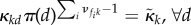
where are the molecular amounts of different types. Assume the space is subdivided into D separate compartments, with counting molecular amounts in compartment d and with counting the total amount of different molecular types in the whole space. We use the same system of reactions in each compartment, but with possibly different chemical constants κ_kd (which also allows for some reactions to be absent).

Example 2.1. —

(Signalling proteins/shared pathway, SP.) Consider a system in which two different proteins A and B are produced from a transcription factor R and are degraded, and when A and B are combined together, they create a product P of interest

The reaction rates for the system in compartment d are

Assume that movement of molecules relocates them individually from one compartment to another. Specific details of the stochastic movement do not have to be precise, because only the long-term distribution of types (π₁(d), … π_m(d)) with will be important for our analysis (not necessarily identical for different types of molecules).

If space was not compartmentalized and the whole system had the same biochemical reactions, the dynamics in would have mass-action rates λ_k = λ_kd using chemical constants κ_k = κ_kd. In space that is compartmentalized but in which the motility of the molecules is faster than any reaction fluctuations, the dynamics in the total amount is equivalent (in the sense of distributions of the resulting stochastic process) to that in a system that is not compartmentalized and has mass-action rates λ_k using averaged chemical constants (theorem 3.7 and corollary 3.8 of [23])

2.1

The system with extremely rapid molecular motility is called well-stirred, and in this case, the dynamics of is simple because it is autonomous. In contrast, when molecular motility is not as rapid then, from the point of view of reaction dynamics, compartments are isolated, and the dynamics of depends on the individual dynamics of all .

Comparing rates of reactions for the total amount of molecules when motility is fast to when it is slow cannot be done in general (except when there is only inflow and unimolecular reactions). If a heterogeneous system starts with completely colocalized molecules, bimolecular reactions have an instantaneous advantage (are more frequent) in the isolated case. If a system starts with pairs of interacting molecules localized in completely distinct compartments, rapid motility gives bimolecular reactions an advantage. However, these advantages cannot hold in any extended window of time, as molecular movement will decorrelate the co- or anti-localization of interacting molecules.

2.2. Stochastic compartment model of chemical reaction system with fluctuations on multiple timescales

Many biochemical reaction systems have fluctuations of relative amounts of molecules happening on multiple timescales. Suppose we can separate the molecular types in the system into those whose fluctuations are effectively on a longer timescale (call them ‘slow’ types ) and those whose fluctuations are on a shorter timescale (call them ‘fast’ types ). Effective here means that fluctuations (net changes) are of the same order of magnitude as the abundance of this molecular type.

This separation of timescales can happen in a number of different ways (via combinations of molecular abundances and orders of magnitude of chemical constants (see [19,20,22,23]). For the sake of simplicity, we consider here the most common way: if a molecular type is present in high abundance (given in terms of a scaling parameter N), then it will need (at least) in the order of N reactions to have an effective change, and will be a ‘slow’ type; if a type is present in small abundance (relative to N), then it will need (only) one reaction to have an effective change, and will be a ‘fast’ type. Let

denote the vectors of rescaled amounts for slow and fast fluctuating molecular types in compartment d, and

the rescaled total amounts over all compartments. Dynamics will have two timescales if any reactions using slow molecular types affect the amount of fast molecular types and vice versa. The dynamics of fast species follows a fast fluctuating Markov chain with dominant rates of O(N). The dynamics of slow types will be well approximated by a system of ordinary differential equations and diffusion fluctuations of size (theorem 2.11 of [21] and examples of [19]). For the derivation of the differential equation driving the slow species, a quasi-steady-state assumption is used. On the fast timescale, is approximately constant, and therefore, converges quickly into their reaction equilibrium, which we call . Then, the effective reaction rate for the slow species based upon the kth reaction is 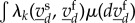. Finally, these effective rates lead to the differential equation

for some function ϕ.

Example 2.2. —

(SP continued.) Suppose the abundances of the transcription factor R and the produced protein P are high, O(N), whereas the abundances of proteins A and B are low, O(1), and suppose chemical constants satisfy , for k = 1, 5, 6, 7 and for the rest j = 2, 3, 4, 8. This implies that fluctuations of rescaled amounts of the transcription factor and of the product are slow, and the fluctuations of proteins V_d,A = X_d,a, V_d,B = X_d,B are fast. The fast species are changed by reactions k = 3, 4, 5, 6, and its fluctuations are produced by a first-order subsystem (k = 7 does not change molecular amounts of A,B). On a short timescale, the rescaled abundance of slow species R has approximately no effective change, so if we condition on the value of V_d,R = v_d,R being constant, the fast production and degradation of A, B in compartment d is approximately a birth–death Markov chain with reaction equilibrium μ_d of independent Poisson distributions for X_d,A and X_d,B with parameters v_d,Rκ_3d/κ_5d and v_d,Rκ_4d/κ_6d, respectively. The dynamics of V_d,R and V_d,P can be approximated by differential equations

where ϕ is the convex function

When movement of molecules is added, multiscale reaction dynamics, as in the example above, requires more complex analysis. Because the reaction dynamics is on different timescales for fast and slow molecular types, movement of molecules also affects them differently. Theoretical results (theorem 3.13 of [23]) show that the only relevant factor is whether the speed of motility of a particular molecular type is faster or slower than its effective reaction dynamics. The speed of molecular types of high abundance—typically these are the slow species—is irrelevant (corollary 3.17 of [23]) as it is somewhat mixing ((ws) or (ss) below), although its stationary distribution plays a role in long-term distributions. However, the speed of fast molecular types in general makes a difference, whereas its stationary distribution plays no role at all (corollary 3.15 of [23]) due to the fact that fast fluctuating amounts change owing to reactions before this distribution is reached. This difference separates systems into the following two cases

• (ws)motility of all molecules is faster than fast fluctuations and the system is well-stirred;
• (ss) motility of ‘fast’ fluctuating molecular species is between the two reaction timescales, and the system is semi-stirred: ‘fast’ fluctuating types are isolated in their compartments prior to reacting on their timescale, whereas ‘slow’ types are well-stirred prior to reacting on their timescale.

Because we scale slow molecular species by the factor N, and we want non-negligible movement on any timescale, we assume the speed of motility of ‘slow’ species at a rate of order with η_s > 0. Then, (ws) corresponds to the speed of motility of ‘fast’ species at a rate of order with η_f > 1, whereas (ss) corresponds to 0 < η_f < 1.

Looking for conditions that will ensure (ws) and (ss) are the same for the dynamics of slow molecules regardless of the speed of fast molecules leads one to consider notions of dynamical homogeneity. If movement is in equilibrium, as is the case in (ws) prior to any reaction dynamics, then each compartment has the same reaction dynamics if

H

for some reference probability distribution π supported on all of 1, … , D. In the special case when this becomes 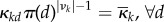. Although the latter condition is more physical (restriction of molecules to smaller compartments leads to their closer proximity and a proportionally higher chance of interactions between two or more molecules) and has often been used to scale the reaction rates to account for unequal volumes of different compartments [11,14,16], this makes sense only if all of the molecular types move and distribute in the same fashion, whereas the condition (H) allows for more general distribution of molecules as long as it is non-degenerate relative to a reference distribution π. (It is clear that it does not allow for any molecular type to localize in a single compartment in the long run, because π_i(d) > 0 is necessary for (H) to hold.)

Dynamical homogeneity is a combined assumption about the chemical constants and long-time movement equilibria in different compartments, and allows for reactivity κ_kd to vary over compartments. If κ_kd are the same for all d, then, (H) will imply π_i = π for any type i involved in a mono-molecular reaction (which then has ν_ik = 1 and ν_jk = 0 for j ≠ i) and π_j = π for any type j that has a bimolecular reaction with type i (which then has ν_ik = ν_jk = 1 and ν_i'k = 0 for all other i’). If movement distributes all molecular types evenly, 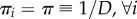, then (H) will imply .

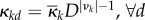The dynamics of fast-fluctuating types is not the same under different motility speeds. However, under specific assumptions, the nature of the fast-fluctuating reaction subsystem can ensure that expected values of in (ws) and (ss) cases can be compared on the timescale of effective change of slow molecules, and that reaction rates for can be approximated by rates in which the fast molecular amounts have been replaced by their expected value (see averaging results detailed in lemmas 2.7, 2.10, 2.12 of [23]).

Example 2.3. —

(SP continued.) In the well-stirred case, movement of A, B molecules is on a faster timescale than reactions (η_A, η_B > 1), whereas in the semi-stirred case, their movement is on slower timescale than production and degradation of A, B, but faster than production of P (0 < η_A, η_B < 1). In (ws) case—no matter if (H) holds—the dynamics of S_R, S_A, S_B, S_P is the same as in a single compartment with chemical constants . Hence, the production of P is approximately a Poisson process with rate

In the (ss) case in each compartment d, the reaction dynamics of A, B is fastest and produces . Movement of molecules then distributes them across compartments according to π_R, π_P, hence the overall production of P is a Poisson process with rate

If (H) holds, we have , for k = 2, 3, 4, , , and hence simple arithmetic shows that

the production rate ϕ of P is the same, regardless of the speed of molecular motility.

3. Overview of results

Theorem 3.1 gives the general result for two timescale reaction systems (see the electronic supplementary material).

Theorem 3.1. —

(Dynamic homogeneity and multiple timescale reaction systems.) If (H) holds and fast fluctuating reactions are of first-order in fast molecular types, then the dynamics of slow molecular types is the same, regardless of whether it is faster (ws) or slower (ss) than fast reaction fluctuations as long as movement of molecules is somewhat faster than the timescale of slow reaction fluctuations.

The assumption of first-order reactions only restricts the subset of reactions that fluctuate on the faster timescale to be linear in terms of fast molecular types, which is true in many important examples (see [25] for a list). It does allow for an arbitrary degree of reactions in the slow molecular types, including their interactions with a single fast molecular type.

The above result holds, regardless of whether the fast fluctuating subsystem has some conserved quantities (as long as we assume that all molecular types combining into a single conserved quantity have the same movement equilibrium), as can be seen in the following classical example of enzymatic kinetics (see [21,26] for other results on the multiscale stochastic fluctuations in this model).

Example 3.2. —

(Michaelis–Menten enzymatic kinetics.) Consider the classical system of enzymatic kinetics consisting of an enzyme E that is needed by a substrate to create an enzyme–substrate complex ES which then gets converted into a product P of interest

The bound enzyme complex is less stable in that the rates releasing the enzyme are an order of magnitude greater than the rate of binding it . The total number of free enzymes and bound enzymes is conserved by the reaction dynamics, denotes the amount of this conserved quantity within a compartment d.

The substrate is often more abundant than the enzyme, and we let and be the rescaled amount of S and P, and V_d,E = X_d,E be the amount of E in compartment d. Given the scaling parameter N, we now express the chemical constants as with . The mass-action rates (in terms of rescaled amounts) are given by As all the reaction rates are high, and the change in enzymes is O(1) per reaction, whereas the change in rescaled substrate is only O(N⁻¹), on the scale of effective changes, the free enzymes and bound enzymes are fast molecular types with fluctuations on a timescale of size N⁻¹, and substrates and products are slow molecular types with fluctuations on a timescale of order 1.

On the timescale of fast fluctuations t, the effective change of the rescaled amount of substrate is negligible, and in any time interval of size o(N) around t can be approximated by v_d,S = V_d,S(t). The fast stochastic behaviour of free and bound enzymes is an Ehrehfest urn with two bins (one for the free and one for the bound state), with transition rates κ_1dv_d,S (from free to bound) and κ_−1d + κ_2d (from bound to free). Its stationary distribution is a simple binomial distribution with parameters n = M_d and p_d = (κ_−1d + κ_2d)/(κ_−1d + κ_2d + κ_1dv_d,S).

When the system is completely well-stirred (speed of E and ES is of the order N^η with η > 1), the sum totals S_S and S_E have the reaction dynamics given by , where is equal to the initial amount of free and bound enzymes in the whole system. The fast fluctuations of S_E have binomial stationary measure μ with , with . On the timescale Nt of slow fluctuations, in any time interval of size around Nt, the rates of effective change of S_S are well approximated by using E_μ[S_E] instead of S_E, and changes in amount N⁻¹ for each reaction have rates With a change of time this stochastic dynamics is well approximated by ordinary differential (or integral) equations

which is the same as what the dynamics of substrates would be in a single compartment system with rate constants given by .

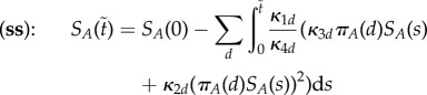
When the system is only semi-stirred (speed of E and ES is of the order N^η with 0 < η < 1), then on the timescale t, the free and bound enzymes are isolated in their compartments. The stationary measure of their fast fluctuations is a product measure of binomials (M_d, p_d) with E_μd[V_E,d] = M_dp_d. On slower timescales, the rates of effective change of V_d,S will be well approximated by using E_μd[V_E,d] instead of V_E,d. On the next timescale N^ηt, molecular movement mixes the total amounts of free and bound enzymes to M_d ∼ binom(M, π_E(d)), and rescaled substrates to V_d,S ∼ δ_πS(d)S_S (the Dirac measure on π_S(d)S_S). This implies that on a slower timescale the reaction rates are averaged with respect to these two movement equilibria. Because the rates are linear in the total amount of free plus bound enzymes, they are replaced by their expectations M_d ≈ π_E(d)M. The rates are not linear in the amount of substrates; however, because we are averaging with respect to a Dirac measure, they are also replaced by V_d,S ≈ π_S(d)S_S. Consequently, on the timescale Nt, the rates of effective change of S_S are approximately where now we have . Under a change of time the dynamics of S_S is close to the deterministic equation

It is not difficult to see that this dynamics is, in general, different from that of in the (ws) case. However, when the compartments are homogeneous in the sense of (H), then the (ss) case (after multiplying both the numerator and denominator by π_E(d)) can easily be shown to reduce to the same equation as in the well-stirred case.

Because notions of dynamic homogeneity do not allow for long-run localization of any of the molecular types (), we consider relaxing their assumptions by focusing only on the dynamics of the fast subsystem with the slow molecular types held constant. In this case, compartments have the same stochastic dynamics of the fast subsystem if

Hfast

for some reference distribution π supported on all of {1, … , D}. In the case , , where the index in the summation or the product above is only over the fast molecular types. This only prohibits fast species from localizing in a single compartment in the long run, allowing for an arbitrary localization of the slow ones.

In the (ws) case, the distribution of slow molecular types is first averaged with respect to movement distribution of the fast ones, followed by reaction dynamics. In the (ss) case reaction, dynamics happens first in each compartment individually, followed by summing of results. Partial homogeneity of fast molecular types (H_fast) will ensure that summing over compartments is equivalent to averaging with respect to π for each compartment in the overall expected change 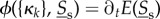of slow molecular types.

Example 3.3. —

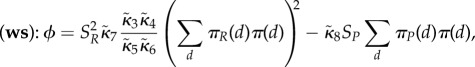
(SP continued.) If we assume (H_fast) holds, then , for k = 2,3,4, , , , . Hence, , for k = 2,3,4, , , , and . Consequently, the (ws) case becomes

whereas the (ss) case becomes

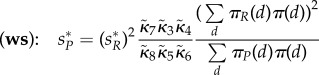
Simple use of Jensen's inequality now shows that ϕ(S_R, S_P) is greater in the (ss) than in the (ws) case, with equality iff π_R ≡ 1/D. The highest production rate of P occurs when the movement of molecules is slow and if the reference measure is as close to π ≡ δ_d* as possible (recall the constraint ), where d^* is chosen as argmax {π_R(d)}. In other words, the proteins A and B should be close to colocalized in the compartment with the maximal average value of the transcription factor R. These conclusions were already observed in Batada et al. [3] using single molecule diffusion calculation.

In the long run, the rescaled abundance of R will converge to an equilibrium regardless of the speed of molecular motility. On the other hand, the production of P will settle into an equilibrium in (ws) case

or in the (ss) case

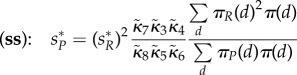to which the same conclusions as above apply. The ratio of equilibria in the (ss) and (ws) cases is given as . See also figures 1 and 2 for some illustrations. For all our simulations, we used the exact sampling method (also called the Gillespie algorithm) for individual reactions via the R-package gillespieSSA by Mario Pineda-Krch.

Figure 1.

We simulated the shared pathway system in D = 2 compartments. We used , π_A(1) = π_A(2) = π_B(1) = π_B(2) = 0.5 (note that these choices fulfil (H_fast) with π(d) = 1/D), together with π_R(1) = 0.9, π_R(2) = 0.1. (Note that in this case, no matter what π_P is.) In the simulations, we used N = 1000. We have that s_P = 2 for (ws), whereas for (ss). Migration rate for R is N^0.5. Dashed lines give theoretical values for equilibria.

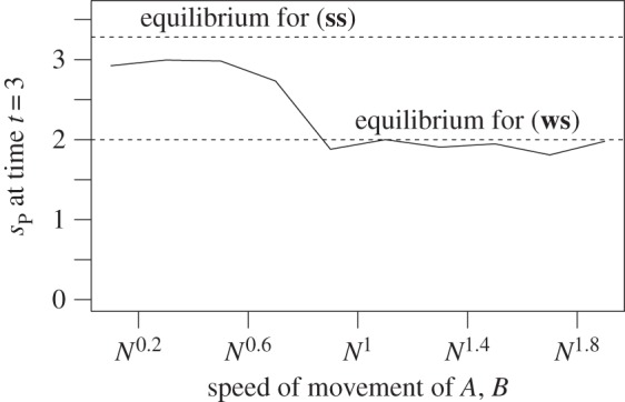
Figure 2.

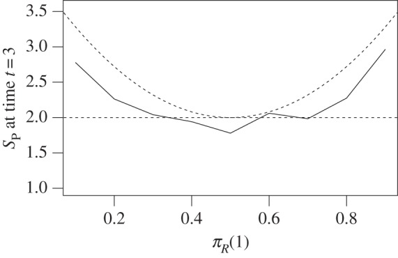
We simulated the shared pathway system in two compartments and different movement equilibria of R. The same parameters as in figure 1 were used, except we fixed speed of movement of A, B to N^0.5 and π_R varies along the x-axis. Dashed lines represent theoretical values for equilibria.

Next result gives a general conclusion for two time-scale systems under (H_fast) and some additional conditions (see the electronic supplementary material).

Theorem 3.4. —

(Fast-dynamic homogeneity and total changes in system.) If (H_fast) holds and fast fluctuating reactions are first-order in fast molecular types, then

1. The change in the expected value of is lower in the (ws) than in the (ss) case when ϕ is convex, whereas the opposite holds when ϕ is concave. Only if , or if ϕ is linear, are the (2s) and (ss) cases the same.

2. The extremal value of ϕ (maximal for convex, minimal for concave) in this case is achieved when in the long run is as close as possible to being localized in a single compartment for which is maximal.

Positive and negative feedback loops are inherent in much of cell regulation (see reference [27] for a survey of control in systems biology). Spatial heterogeneity can have a mollifying or enhancing effect on their mechanisms, even when a protein is spatially localized, as shown in a simple model of mutual activation.

Example 3.5. —

(Self-regulatory feedback mechanisms). Consider the system in which a protein A is self-regulated by its own product B via a negative feedback mechanism

A positively self-regulated system is similar except that the first reaction is replaced by . Suppose the rates of creation and degradation of the product B are much faster than the other reactions, and that the protein A is generally much more abundant than B. We will assume that movement of A and B is such that in the long run the protein A can be localized, but its product B is distributed evenly over the space. For some scaling parameter N, we let , and be the rescaled amounts of molecules, and express leaving as is. The mass-action rates (in terms of rescaled amounts) are given by

On a timescale of order 1, the relative change of rescaled amounts V_d,A is negligible, whereas the fluctuations of V_d,B are rapid with equilibrium that conditionally on V_d,A = v_d,A is Poisson with mean (κ_3d + κ_2dv_d,A)/κ_4d. On a longer timescale of order N, the expected change of V_d,A is well approximated by the equation

with the concave function

When movement of molecules has speed of order N^η with η > 1, then the total amount of rescaled A molecules on the timescale approximately satisfies

with rate constants

When movement of molecules has speed of order N^η with 0 < η < 1, then molecules of B are isolated in their compartments prior to their fluctuations. The total amount of rescaled A molecules is then obtained as a sum of amounts in individuals compartments, on the timescale approximated by

If the system is partially homogeneous, so that reaction constants and distribution of B molecules satisfy (H_fast), then , and . Assume then in (ws) case

and in (ss) case

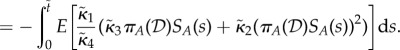
Now, concavity of ϕ implies that the gradient of change of is greater (it is smaller in absolute value) in the well-stirred than in the semi-stirred case. Only in the special case when the two dynamics reduce to the same. For the positive feedback system, the gradient of change has the exact same form except with a positive sign. Its convexity implies that the gradient of change of is smaller in the well-stirred than in the semi-stirred case. Importantly, all above results are completely independent of the long-run spatial distribution π_A of A molecules. In figure 3, we have implemented the negative feedback example in the (ws) and (ss) case, which gives an illustration of the fact that A degrades faster if B moves slowly.

Figure 3.

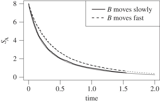
The simulation of the negative feedback system shows that A molecules are less abundant if B molecules move slowly (i.e. η < 1). We chose D = 4, N = 1000, π = unif, π_A(1) = 5/8, π_A(2) = π_A(3) = π_A(4) = 1/8. For slow movement of B, we have η = 0.6, whereas η = 1.3 for fast B-movement.

4. Discussion

In cellular networks, stochasticity of reactions and a heterogeneous environment both affect concentration fluctuations. Stochastic averaging methods provide powerful ways to rigorously approximate spatially heterogeneous reaction systems fluctuating on multiple timescales with molecular movement between compartments. Even if the spatial component of a cell is simplified by using a compartment model, full calculations accounting for changes owing to both effects are cumbersome. Our results provide a simple method for making conclusions for a general class of spatially heterogeneous systems with reactions on multiple timescales based on differential equations for the sum totals of each slowly fluctuating molecular types within the system. They provide answers to the question of sensitivity of long-term dynamics of a downstream quantity of interest with respect to molecular motility: only the speed of movement of highly fluctuating molecular types is relevant and the level of nonlinearity is reduced in case this speed is greater than their fluctuations. Our results also rigorously show the effect that the long-run spatial distribution of molecules has. Localization of slowly fluctuating molecular types and their even distribution over compartments are two extremal measures achieving opposite effects in the behaviour of the overall dynamics of interest. While our approach results in differential equations for slowly fluctuating molecular types based on quasi-steady-state assumptions, we could also ask for the precise form of fluctuations of the sum totals of slow molecular types. More effects can be expected here, because slower movement of slow molecular types may result in higher fluctuations.

Our assumption (H_fast) models a situation where space is fully homogeneous from the viewpoint of fast fluctuating species, whereas slow species may be localized in space. Such a situation occurs when small molecules react fast and have high motility through space, whereas slow fluctuating molecules belong to specific cellular compartments and have low motility and are therefore either colocalized (if they belong to the same compartment) or isolated (if they belong to different compartments). In the example of the SP, our results under (H_fast) can be understood intuitively: if RNA is moving slowly and makes molecules of A and B which together produce P, the production of the latter is more efficient if A and B move slower than they produce P, because production of P requires colocalized molecules of A and B. In the example of Michaelis–Menten kinetics, we found the opposite behaviour. Here, fast movement of molecules leads to faster production of the product P from the substrate S. This can also be explained intuitively: enzymes turn S into P molecules via the enzyme/substrate complex; in the extreme case, S is completely localized in one compartment, enzymes can only turn them into product there; when an enzyme moves slowly and moves away from the compartment, it can, at most, release one P molecules and then has to travel for a long time until it returns to the compartment where it can turn S into P; if, however, the enzyme moves quickly, its travel time before reaching the efficient compartment is smaller and, therefore, production of P is more efficient. Our results give the analytical framework for studying spatially distributed multiscale systems, and rigorously justify such intuitive conclusions.

Funding statement

This study was partially supported by NSERC Discovery grant no. 346197.

References

- 1.Batada NN, Shepp LA, Siegmund DO. 2004. Stochastic model of protein–protein interaction: why signaling proteins need to be colocalized. Proc. Natl Acad. Sci. USA 101, 6445–6449. ( 10.1073/pnas.0401314101) [DOI] [PMC free article] [PubMed] [Google Scholar]
- 2.Lingwood D, Simons K. 2010. Lipid rafts as a membrane-organizing principle. Science 327, 46–50. ( 10.1126/science.1174621) [DOI] [PubMed] [Google Scholar]
- 3.Strahl H, Bürmann F, Hamoen LW. 2014. The actin homologue MreB organizes the bacterial cell membrane. Nat. Commun. 5, 3442 ( 10.1038/ncomms4442) [DOI] [PMC free article] [PubMed] [Google Scholar]
- 4.Di Rienzo C, Gratton E, Beltram F, Cardarelli F. 2013. Fast spatiotemporal correlation spectroscopy to determine protein lateral diffusion laws in live cell membranes. Proc. Natl Acad. Sci. USA 110, 12 307–12 312. ( 10.1073/pnas.1222097110) [DOI] [PMC free article] [PubMed] [Google Scholar]
- 5.Ghaemmaghami S, Huh W-K, Bower K, Howson RW, Belle A, Dephoure N, O'Shea EK, Weissman JS. 2003. Global analysis of protein expression in yeast. Nature 425, 737–741. ( 10.1038/nature02046) [DOI] [PubMed] [Google Scholar]
- 6.Elowitz MB, Levine AJ, Siggia ED, Swain PS. 2002. Stochastic gene expression in a single cell. Science 297, 1183–1186. ( 10.1126/science.1070919) [DOI] [PubMed] [Google Scholar]
- 7.Swain PS, Elowitz MB, Siggia ED. 2002. Intrinsic and extrinsic contributions to stochasticity in gene expression. Proc. Natl Acad. Sci. USA 99, 12 795–12 800. ( 10.1073/pnas.162041399) [DOI] [PMC free article] [PubMed] [Google Scholar]
- 8.Kaern M, Elston TC, Blake WJ, Collins JJ. 2005. Stochasticity in gene expression: from theories to phenotypes. Nat. Rev. Genet. 6, 451–464. ( 10.1038/nrg1615) [DOI] [PubMed] [Google Scholar]
- 9.Raser JM, O'Shea EK. 2005. Noise in gene expression: origins, consequences, and control. Science 309, 2010–2013. ( 10.1126/science.1105891) [DOI] [PMC free article] [PubMed] [Google Scholar]
- 10.Kalay Z, Fujiwara TK, Kusumi A. 2012. Confining domains lead to reaction bursts: reaction kinetics in the plasma membrane. PLoS ONE 7, e32948 ( 10.1371/journal.pone.0032948) [DOI] [PMC free article] [PubMed] [Google Scholar]
- 11.Mugler A, Tostevin F, ten Wolde PR. 2013. Spatial partitioning improves the reliability of biochemical signaling. Proc. Natl Acad. Sci. USA 110, 5927–5932. ( 10.1073/pnas.1218301110) [DOI] [PMC free article] [PubMed] [Google Scholar]
- 12.Andrews SS, Bray D. 2004. Stochastic simulation of chemical reactions with spatial resolution and single molecule detail. Phys. Biol. 1, 137–151. ( 10.1088/1478-3967/1/3/001) [DOI] [PubMed] [Google Scholar]
- 13.van Zon JS, ten Wolde PR. 2005. Simulating biochemical networks at the particle level and in time and space: Green's function reaction dynamics. Phys. Rev. Lett. 94, 128103 ( 10.1103/PhysRevLett.94.128103) [DOI] [PubMed] [Google Scholar]
- 14.Fange D, Berg OG, Sjöberg P, Elf J. 2010. Stochastic reaction–diffusion kinetics in the microscopic limit. Proc. Natl Acad. Sci. USA 107, 19 820–19 825. ( 10.1073/pnas.1006565107) [DOI] [PMC free article] [PubMed] [Google Scholar]
- 15.Melo E, Martins J. 2006. Kinetics of bimolecular reactions in model bilayers and biological membranes: a critical review. Biophys. Chem. 123, 77–94. ( 10.1016/j.bpc.2006.05.003) [DOI] [PubMed] [Google Scholar]
- 16.Kang H-W, Zheng L, Othmer HG. 2012. A new method for choosing the computational cell in stochastic reaction–diffusion systems. J. Math. Biol. 65, 1017–1099. ( 10.1007/s00285-011-0469-6) [DOI] [PMC free article] [PubMed] [Google Scholar]
- 17.Flegg MB, Chapman SJ, Erban R. 2012. The two-regime method for optimizing stochastic reaction–diffusion simulations. J. R. Soc. Interface 9, 859–868. ( 10.1098/rsif.2011.0574) [DOI] [PMC free article] [PubMed] [Google Scholar]
- 18.Gillespie DT, Hellander A, Petzold LR. 2013. Perspective: stochastic algorithms for chemical kinetics. J. Chem. Phys. 138, 170901 ( 10.1063/1.4801941) [DOI] [PMC free article] [PubMed] [Google Scholar]
- 19.Ball K, Kurtz T, Popovic L, Rempala G. 2006. Asymptotic analysis of multiscale approximations to reaction networks. Ann. Appl. Prob. 16, 1925–1961. ( 10.1214/105051606000000420) [DOI] [Google Scholar]
- 20.Kang HW, Kurtz T. 2013. Separation of time-scales and model reduction for stochastic reaction models. Ann. Appl. Prob. 23, 529–583. ( 10.1214/12-AAP841) [DOI] [Google Scholar]
- 21.Kang H-W, Kurtz T, Popovic L. 2014. Central limit theorems and diffusion approximations for multiscale Markov chain models. Ann. Appl. Prob. 24, 721–759. ( 10.1214/13-AAP934) [DOI] [Google Scholar]
- 22.Franz U, Liebscher V, Zeiser S. 2012. Piecewise-deterministic Markov processes as limits of Markov jump processes. Adv. Appl. Prob. 44, 719–748. ( 10.1239/aap/1346955262) [DOI] [Google Scholar]
- 23.Pfaffelhuber P, Popovic L. In press. Scaling limits of spatial chemical reaction networks. Ann. Appl. Prob. [Google Scholar]
- 24.Kurtz T. 1992. Averaging for martingale problems and stochastic approximation. In Applied stochastic analysis (New Brunswick, NJ, 1991), Vol. 177, Lecture Notes in Control and Information Sciences Series (eds Karatzas I, Ocone D.), pp. 186–209. Berlin, Germany: Springer. [Google Scholar]
- 25.Gunawardena J. 2012. A linear framework for time-scale separation in nonlinear biochemical systems. PLoS ONE 7, e36321 ( 10.1371/journal.pone.0036321) [DOI] [PMC free article] [PubMed] [Google Scholar]
- 26.Kou S. 2001. Stochastic networks in nanoscale biophysics: modeling enzymatic reaction of a single protein. J. Am. Stat. Assoc. 103, 961–975. ( 10.1198/016214507000001021) [DOI] [Google Scholar]
- 27.Sontag E. 2005. Molecular systems biology and control. Eur. J. Control 11, 396–435. ( 10.3166/ejc.11.396-435) [DOI] [Google Scholar]
Associated Data
This section collects any data citations, data availability statements, or supplementary materials included in this article.