

Abstract
Being multilayered and anisotropic, biological tissues such as cardiac and arterial walls are structurally complex, making full assessment and understanding of their mechanical behavior challenging. Current standard mechanical testing uses surface markers to track tissue deformations and does not provide deformation data below the surface. In the study described here, we found that combining mechanical testing with 3-D ultrasound speckle tracking could overcome this limitation. Rat myocardium was tested with a biaxial tester and was concurrently scanned with high-frequency ultrasound in three dimensions. The strain energy function was computed from stresses and strains using an iterative non-linear curve-fitting algorithm. Because the strain energy function consists of terms for the base matrix and for embedded fibers, spatially varying fiber orientation was also computed by curve fitting. Using finite-element simulations, we first validated the accuracy of the non-linear curve-fitting algorithm. Next, we compared experimentally measured rat myocardium strain energy function values with those in the literature and found a matching order of magnitude. Finally, we retained samples after the experiments for fiber orientation quantification using histology and found that the results satisfactorily matched those computed in the experiments. We conclude that 3-D ultrasound speckle tracking can be a useful addition to traditional mechanical testing of biological tissues and may provide the benefit of enabling fiber orientation computation.
Keywords: 3-D ultrasound speckle tracking, Biaxial mechanical testing, Constitutive relations, Soft tissue mechanics
INTRODUCTION
Biological samples such as myocardium and great arterial vessel walls are known to have complex tissue architectures (Arts et al. 2001; Glagov et al. 1992; Scollan et al. 2000) and complex mechanical responses to loads (Stuber et al. 1999). Knowledge of their mechanical behavior aids in understanding their function and remodeling characteristics, and can help to improve disease treatment and management. It also provides an instructive guide for tissue engineering during the development of replacement tissues. For these reasons, there is continued interest in the characterization of soft tissue mechanics (Holzapfel and Ogden 2009).
The current standard method for measuring the passive mechanical properties of biological samples uses multiaxial loading and strain measurements (Gleason et al. 2007; Humphrey et al. 1990c; Sacks 2000). The strains of the tissue are usually measured by visually tracking markers placed on the surface of the samples via conventional cameras. One limitation of this method is that it provides only 2-D strains on the surface of the sample; it does not provide strains beneath the surface. Ultrasound speckle tracking (Meunier 1998; O’Donnell et al. 1994; Ophir et al. 1991), in its 3-D version (3-DUST) (Chen et al. 2005), can be employed to overcome this difficulty, because it can non-invasively track 3-D deformations in a 3-D volume in samples that are optically opaque and have a non-negligible thickness. In this article, we describe the feasibility of one such instance.
We present the details of a new method for mechanical testing of biological samples using concurrent 3-DUST and biaxial testing. The backbone of the method is an algorithm used to compute the strain energy function from the stress and strain tensors using non-linear curve fitting, which was validated with in silico finite-element analysis (FEA). We illustrate the experimental feasibility of the method by testing on rat myocardium. Strain energy functions computed from our experimental data were compared with measurements reported by others.
METHODS
All animal studies were approved by the University of Pittsburgh’s Institute Animal Care and Use Committee. Figure 1 illustrates the overall methodology. We performed biaxial testing of samples and used 3-D ultrasound speckle tracking to obtain the full 3-D strain tensor to describe deformation. We use forces measured with the biaxial tester to compute diagonals of the stress tensor. Using the two pieces of data, we assume an initial guess of the mechanical properties of the sample and perform an iterative non-linear curve fitting to refine the mechanical property parameters. Details are given below.
Fig. 1.

Schematic for computation of the material model (strain energy function coefficients) and spatially varying fiber orientation. Trimmed samples were placed into a saline bath for concurrent 3-D ultrasound imaging and biaxial testing. Three-dimensional strain tensors are derived from 3-D ultrasound speckle tracking of ultrasound images; diagonals of the stress tensor are computed by dividing measured force by cross-sectional area. The strain energy function coefficients are then computed from stress and strain values using an iterative non-linear curve-fitting algorithm that minimizes the difference in measured and computed stress tensor diagonals. With each iteration, fiber orientations are computed based on the non-converged strain energy function, also by matching computed and measured stresses, such that the optimization process will also seek least-squares solutions to the originally unknown fiber orientations.
Biaxial mechanical testing and ultrasound scanning
The experimental setup is illustrated in Figure 2a and b, and the direction convention in Figure 2c. Samples were tested with a commercial biaxial tester (BioTester, CellScale, Waterloo, ON, Canada), and concurrent ultrasound imaging was performed using a 30-MHz linear array transducer (MS400, VisualSonics, Toronto, ON, Canada) connected to a high-frequency ultrasound system (Vevo 2100, VisualSonics). The system has 256 channels, and the transducer has 256 elements. Each element has a lateral width of 0.060 mm and elevational width of 2.0 mm. Images recorded had 784 axial samples over a distance of 12 mm and 444 lateral scan lines over a distance of 13.36 mm. The transducer, as described by the manufacturer, had an axial resolution of 50 μm and lateral resolution of 110 μm.
Fig. 2.

Experimental setup. (a) Schematic of the setup. (b) Aerial view of the sample in the biaxial tester. The rat left ventricular free wall sample was trimmed into a rectangular sample approximately 10 × 10 mm and tested with a biaxial mechanical tester. A system of pulleys ensures the distribution of stresses along the edges of the sample. Three-dimensional ultrasound speckle images were gathered at each quasi-static stretch state by traversing a high-frequency 2-D linear-array transducer in the out-of-plane direction with a linear stepper motor and scanning the sample at regular spatial intervals. Forces imposed on the sample were measured by force gauges attached to the biaxial actuator arms. (c) Axis coordinate convention used in the present study.
The left ventricular free wall of a rat heart was excised and trimmed to a 10 × 10-mm block (approximately 3 mm thick) before being tested in the biaxial tester. The samples were mounted onto the biaxial tester via metal hooks. A system of pulleys distributed loads evenly among the four hooks on each edge of the sample. Sample mounting was done such that the apex–base axis of the myocardium was aligned with the elevational axis of the ultrasound-biaxial experimental setup (Fig. 2c), the medial-lateral axis of the myocardium was aligned with the lateral axis of the setup and the trans-luminal axis of the myocardium was aligned with the axial axis of the setup.
A small preload of 3 mN was applied to spread the sample out uniformly. Preconditioning (preparatory stretching of the sample before actual mechanical testing) was then performed from this initial condition to the highest stretch level for three cycles. Three-dimensional ultrasound scans were performed using the 2-D transducer mounted onto a linear actuator motor supplied by the manufacturer. For each 3-D volume acquisition, imaging was performed along 39 planes spaced 0.102 mm apart, using the linear motor to rapidly and sequentially displace the transducer to these 39 positions. As a result, each 3-D volume scan required approximately 4 s. Consequently, a quasi-static biaxial testing protocol was needed: The sample was stretched to consecutively higher stretch levels, and at each stretch level, the sample was held stationary for 6 s for ultrasound imaging. Between stretches, the sample was relaxed to the initial, low-stress condition for 8 s.
Forces applied to the sample in the two stretch axes were measured with a load cell, and the diagonals of the stress tensor were computed by dividing by the cross-sectional area, which was measured from ultrasound images. This was performed at a reference stretch condition. Stresses under other conditions were then computed by updating the stress under the reference condition with the stretch ratios (to account for area changes) and with the measured force. Stress in the third axis, perpendicular to the two biaxial axes was assumed to be zero.
The peak stretch level was set to be approximately 25%. This choice was guided by in vivo observations that the myocardium undergoes 12%–22% strain (Urheim et al. 2000). The peak stresses experienced by the sample were about 80–100 g/cm, comparable to those of previous myocardium biaxial experiments (Humphrey et al. 1990a).
To enable easy fitting of a material model to the ultrasound-biaxial test data, we adopted the “dual-loading protocol,” in which two biaxial tests are performed on the same sample, using different loading conditions for the two tests, and then used measurement data from both tests simultaneously to fit a material model.
Ultrasound speckle tracking
Because the Vevo 2100 ultrasound machine saves raw data in the IQ demodulated format, we exported images in the IQ format. Three-dimensional ultrasound speckle tracking was applied to the reconstructed radio-frequency data to compute the spatially varying three-component displacements over a volume in the sample. The details of the phase-sensitivity 3-DUST algorithm used in this study are described in a previous publication (Chen et al. 2005). Through autocorrelation of the source images, it was found that average speckle size was 0.061 × 0.12 × 0.20 mm in the axial, lateral and elevational directions. The kernel size during the cross-correlation of 3-D speckle tracking was set slightly larger: 0.11 × 0.21 × 0.3 mm in the axial, lateral and elevational directions. According to evaluations by previous investigators (Konofagou and Ophir 1998; Lubinski et al. 1999; O’Donnell et al. 1994; Skovoroda et al. 1994), ultrasound speckle tracking has reliable accuracy.
The 3-D displacements between consecutive frames were accumulated to give the Lagrangian displacements for every frame, all of which were referenced to the prestretch condition. Lagrangian displacements were then used to calculate strains with the equations (Humphrey 2002)
| (1) |
| (2) |
| (3) |
| (4) |
where X is the reference coordinate, x is the deformed coordinate, F is the deformational gradient tensor, C is the right Cauchy–Green deformation tensor, ε is the Green strain and I is the identity matrix. This formal treatment of deformation is used, as we needed to employ finite strain theory instead of infinitesimal strain theory, because we observe large strains, and infinitesimal theory is inaccurate for such a scenario. Either the Almansi strain (deformation normalized by original lengths) or the Green strain (deformation normalized by final lengths) could have been used in our formulation, but we have chosen to use the Green strain out of convenience. Biaxial testing was conducted with a prespecified actuator displacement rather than prespecified strain values, and both stresses and strains were computed after the testing.
Modeling the mechanical property
We modeled the mechanical property of the test samples with established mathematical formulation, and refer readers to Humphrey (2002:Ch 3). Our goal is to fit the experimental test data to this mechanical property model and derive the values of the model parameters.
The constitutive relations equation (relating stresses and deformation) has the form
| (5) |
where W is the SEF, σ is the Cauchy stress and p is the Lagrangian multiplier that enforced incompressibility. The SEF is the mathematical representation of the mechanical property of the test sample. We have chosen to use SEF in the form derived previously (Humphrey and Yin 1987; Humphrey et al. 1990b), which consists of terms to describe stiffness of the base matrix and stiffness of embedded fibers, which are oriented in one particular direction. According to the formulation by Humphrey et al. (1990b), W = W (I1, I4), where I1 and I4 are the first and fourth invariants of deformation (Humphrey 2002):
| (6) |
| (7) |
where N is the unit vector in the orientation of the embedded fiber. A is also the stretch ratio in the direction f the fiber. This leads to the form for dW/dC due to chain rule
| (8) |
where ⊗ is the dyadic product or outer product, where ui⊗vj = uivj. Thus, eqn (5) can be expressed as (Humphrey et al. 1990c)
| (9) |
Two SEF formulations were investigated in the present study for modeling the material property of the myocardium. These SEFs were assumed to be constant for every point within the sample and were assumed to be independent of deformation. The first is (Humphrey and Yin 1987)
| (10) |
where c, b, A and a are the four coefficients defining the SEF. The second is (Humphrey et al. 1990c)
| (11) |
where c1–c5 are the SEF coefficients.
In the current implementation, which serves as a foundation to the 3-DUST mechanical testing technique, it is assumed that the fiber orientations are only in the lateral-elevational plane (Fig. 2c), and thus, fibers can be described by a single angle parameter at every location. We note that it is possible to model truly 3-D fiber orientations using two angle parameters instead of one, but this will be at the expense of additional computational time. The fiber orientations were assumed to be fixed with respect to the base matrix, but were allowed to change directions because of deformation. The fiber orientation at any one point was assumed to be independent of fiber orientations at any other location.
Non-linear curve-fitting algorithm computation
We had measurements of stresses in the three axes and, thus, could use three equations from eqn (9), relating σ11, σ22 and σ33, and to deformation (the first, second and third axes were the lateral, elevational and axial axes). We use the σ33 equation to remove the Lagrangian multiplier, p, from the other two.
The SEF coefficients were computed from the strain and stress tensors through an iterative non-linear curve-fitting method that minimizes the sum-squared-error of the stress tensor diagonals:
| (12) |
Here, and are the stress tensor diagonals along the ith axis: The former was computed based on experimental force and cross-sectional areas measurements, and the latter was computed by the non-linear curve-fitting algorithm, using the Trust Region Reflective algorithm (More and Sorensen 1983). The parameters being optimized by the algorithm are only the SEF parameters, and the initial guesses of SEF values were based on previous studies (Humphrey et al. 1990c).
With each iteration of the curve-fitting algorithm, however, we have a separate optimization problem to solve for the spatially varying fiber orientations. At any one location, the fiber orientation was computed from the SEF (not yet converged), the strain tensor and the diagonals of the stress tensor, using the simplified form of eqn (9) (without p). Multiple equations (from two biaxial tests and from multiple stretch levels within each biaxial test) were used to find one single fiber orientation value that minimizes the measured and computed stress diagonals, using a “brute-force” approach, where 300 fiber orientations covering all possible ranges were tested and the optimal one was adopted.
In the Trust Region Reflective curve fitting, all four SEF parameters were optimized at the same time, but on completion of the curve fitting, we undertook extensive further optimization to minimize the possibility that the solution was in a local minimum instead of the global minimum. We carried out a series of perturbation experiments. Within each experiment, one of the SEF coefficients was perturbed by doubling or halving its value, and the curve-fitting operation was repeated. Perturbation experiments were performed for all four SEF coefficients sequentially, for which the coefficient was doubled and also where the coefficient was halved. If none of the perturbation experiments produced a lower residual than the initial curve fitting, the initial result was assumed to have reached the global minimum; otherwise, the entire perturbation exercise was restarted with the new solution of lower residual. Fiber orientations, which were initially unknown, were recovered iteratively through the curve fitting as well.
To evaluate the goodness of fit of the final SEF results, we used the second moments ( ) of ( ).
Finite-element simulation and validation
Finite-element analysis was performed to validate our non-linear curve-fitting algorithm. FEA of biaxial testing was performed using phantom SEF parameters, chosen to be close to the values in other studies (Humphrey and Yin 1987). From FEA results, only tissue displacements and imposed stresses (and not the phantom SEF or fiber orientation values) were retained for analysis with the non-linear curve-fitting algorithm, which then re-computed the SEF and fiber orientations. In essence, we blinded the algorithm to the originally assumed SEF and fiber orientation and tested whether the algorithm can back-compute these values using only the tissue displacements and imposed stresses. We then compared the re-computed SEF and fiber orientations with the originally assumed values to see if the algorithm could accurately retrieve them.
Finite-element analysis was performed using a commercial finite-element simulation package (COMSOL, Comsol, Burlington, MA, USA) and featured a rectangular tissue sample (dimensions: 30 × 30 × 3 or 30 × 30 × 10 mm in lateral, elevational and axial axes) being stretched biaxially with progressively greater stress. Uniform stresses were imposed on the four side boundaries (lateral and elevational boundaries), whereas the top and bottom surface boundaries (axial boundaries) were assumed to be stress free. A total of 12 cases of homogeneous fiber orientations, with fiber angles ranging from 0 to 90° (from the lateral axis), were simulated. Two cases of inhomogeneous fiber orientations were simulated: The first featured fiber orientation varying from 0 to 90° along the lateral axis (Fig. 3a); and the second featured fiber orientation varying from 0 to 57° along the axial axis (Fig. 3b). The simulated tissue sample was meshed into approximately 50,000 tetrahedral elements for the simulations.
Fig. 3.

Three-dimensional models used in finite-element simulations to validate the non-linear curve-fitting algorithm used for computing strain energy function coefficients. Arrows indicate the orientation of fibers at specific locations within the sample volume. The first model (a) has fiber orientations varying with the lateral axis, whereas the second model (b) has fiber orientations varying with the axial axis.
Fiber orientation quantification with histology
After the biaxial mechanical test, the same rat left ventricular wall sample was fixed in formalin and analyzed with standard Masson trichrome stain to obtain fiber orientations. Stained slides were digitally scanned with Nikon Super Coolscan 9000 ED (Nikon, Melville, NY, USA) at a 6.3-μm pixel resolution and analyzed with fast Fourier transformation using custom-written MATLAB (The Mathworks, Natick, MA, USA) programs at multiple points on the lateral-axial plane. Metal hooks were visible in the ultrasound images, and holes made by hooks in the tissues were identifiable on the histologic images. These were used as landmarks to geometrically register histology images to ultrasound images.
Fiber orientations quantified with histology were compared with those computed from the non-linear curve-fitting algorithm from 3-DUST biaxial experiments.
RESULTS
In silico validation of non-linear curve-fitting algorithm
Finite-element simulations revealed that the nonlinear curve-fitting algorithm could accurately compute fiber angles and SEFs from only tissue displacements and boundary stresses, for FEA cases with homogeneous fiber angles (Table 1). Averaged over all 12 cases, errors in SEFs were less than 0.3%, whereas errors in fiber orientation were less than 0.5°. The results for the cases with inhomogeneous fiber orientation are summarized in Table 2 and Figure 4. It was found that for samples with significantly inhomogeneous fiber orientation, use of data from two different loading conditions for concurrent entry into the non-linear curve-fitting algorithm resulted in better accuracy and convergence. Having two loading conditions is equivalent to mechanically testing the same sample twice with different loading patterns and then concurrently inputting tissue displacements and boundary stresses from both tests into the algorithm to compute the SEF. It should be noted that the fiber orientation and SEF parameters were assumed not to change between the two loading conditions. As outlined in Table 2, for cases in which only one loading condition was entered, the third and fourth SEF coefficients (a and A in eqn 10, respectively) can have large errors, but in cases where two loading conditions were entered, this error was greatly reduced. Figure 4 illustrates the fiber orientation computed over one lateral-axial plane for the two inhomogeneous fiber orientation cases, revealing reasonable agreement between the algorithm-computed fiber orientations and the actual fiber orientations.
Table 1.
Validation of the non-linear curve-fitting computation algorithm for the first strain energy function (eqn 10) for the homogeneous fiber orientation case*
| Case | Actual fiber angle | Computed fiber angle | Computed strain energy function coefficient
|
|||
|---|---|---|---|---|---|---|
| b (Pa) | c | A (Pa) | A | |||
| 1 | 0.00 | 20.32 | 100.0 | 14.00 | 100.0 | 55.00 |
| 2 | 2.86 | 2.40 | 100.0 | 14.00 | 99.95 | 54.99 |
| 3 | 5.73 | 5.40 | 100.0 | 14.00 | 99.80 | 54.97 |
| 4 | 17.2 | 17.4 | 99.90 | 14.00 | 100.6 | 55.06 |
| 5 | 28.6 | 28.8 | 99.82 | 14.00 | 101.2 | 55.06 |
| 6 | 40.1 | 40.2 | 99.61 | 14.01 | 101.3 | 55.79 |
| 7 | 51.6 | 51.6 | 100.2 | 14.00 | 99.06 | 54.93 |
| 8 | 63.0 | 63.0 | 100.0 | 14.00 | 99.73 | 55.05 |
| 9 | 74.5 | 74.4 | 99.99 | 14.00 | 100.0 | 55.01 |
| 10 | 84.2 | 85.2 | 100.0 | 14.00 | 100.0 | 55.00 |
| 11 | 87.1 | 89.4 | 100.1 | 14.00 | 99.31 | 55.11 |
| 12 | 90.0 | 89.4 | 100.0 | 14.00 | 100.0 | 55.00 |
| Actual strain energy function coefficient
|
||||
|---|---|---|---|---|
| b (Pa) | c | A (Pa) | a | |
| For all fiber angles: | 100.0 | 14.00 | 100.0 | 55.00 |
Only tissue displacement and boundary stress output from finite-element analysis were used in the algorithm, which was used to recompute the strain energy function coefficient and fiber orientation. The re-computed fiber angle and coefficient matched the original values well.
Table 2.
Computation of the SEF using only tissue displacement and boundary stress data output from the finite-element analysis simulations, for the inhomogeneous fiber orientation case (Fig. 3a), employing the first SEF (eqn 7) *
| Computed SEF coefficient
|
||||
|---|---|---|---|---|
| b (Pa) | c | A (Pa) | a | |
| Single-loading condition | ||||
| Case 1: αL = αE | 103.15 | 13.91 | 68.15 | 62.86 |
| Case 2: αL = 1.1αE | 108.07 | 13.71 | 29.00 | 98.36 |
| Dual-loading condition | ||||
| Case 1: αL = 1.05αE; αE = 1.05αL | 99.53 | 14.01 | 105.74 | 53.91 |
| Case 2: αL = 1.1αE; αE = 1.1αL | 100.64 | 13.99 | 104.17 | 52.19 |
| Case 3: αL = 1.15αE; αE = 1.15αL | 99.04 | 14.034 | 118.17 | 50.40 |
| Actual SEF coefficient
|
||||
|---|---|---|---|---|
| b (Pa) | c | A (Pa) | a | |
| For all cases above: | 100.00 | 14.00 | 100.00 | 55.00 |
SEF = strain energy function; αL = stress in lateral direction; αE = stress in elevational direction.
Computation was more accurate when two sets of loading conditions (as opposed to only one set) were used concurrently in the algorithm, which was equivalent to testing the sample twice and then using the displacement and boundary stresses from both tests in the same computation to retrieve the SEF. Results also converged better when two sets of loading conditions were used simultaneously (employing the “dual-loading protocol”).
Fig. 4.

Plot of fiber orientation computed by the non-linear curve-fitting algorithm, using displacement data and boundary stress data from finite-element simulations as inputs, and plot of the true fiber orientation used to perform the simulations, illustrating that the algorithm could retrieve these fiber orientations. Results are displayed for the first finite-element model, where fiber angles vary with the lateral axis (a), and for the second finite-element model, where fiber angles vary with the axial axis (b).
Biaxial ultrasound experiment on rat left ventricular free wall
Figure 5a is a typical real-time force-versus-displacement plot measured by the biaxial tester. The sample was tested with multiple loading cycles, each with a higher displacement and force than the previous. The rat left ventricular sample was tested under the dual-loading protocol, as illustrated in Figure 5b. In Figure 5c and d are sample raw B-mode speckle images.
Fig. 5.

Plots of the loading conditions and the raw speckle images. (a) Plot of real-time force-displacement measurements from one biaxial actuator for preconditioning (black line) and actual testing (gray line), which imposed several stretch cycles to progressively higher quasi-static stretch levels. After each stretching phase, the sample was held stationary, and a set of ultrasound images were acquired. Each black dot represents the average of the first five data points immediately after the beginning of this stationary phase and is the force datum assumed at each imaging point. The quasi-static manner of stretching (black dots) approximates the loading arm of a single fully dynamic stretch cycle, represented by the preconditioning cycle (black line), thus illustrating that stress relaxation did not cause the quasi-static testing to deviate significantly from fully dynamic testing. (b) Plots of the two sets of loading conditions under which the sample was biaxially tested. (c) Representative lateral-axial plane raw ultrasound speckle image of the sample and the hooks attached to the sample. The thick dotted line indicates the location for plotting (d) the representative elevational-axial plane raw ultrasound speckle image of the sample. The thick dotted line indicates the location for plotting (c).
Figure 6 illustrates typical output from the 3-DUST algorithm, which performed 3-D cross-correlation between two consecutive image volumes. The correlation coefficients were generally high (>0.8 at locations where data are used), suggesting that the output had high fidelity. Lateral displacements showed opposite ends moving away from one another, in agreement the tensile motion imposed by the biaxial tester on the sample.
Fig. 6.

Representative outputs from 3-D speckle tracking moving from one stretch state to the next. Correlation coefficient of the cross-correlation (a) and the axial (b), lateral (c) and elevational (d) pixel displacements between these two stretch states.
Non-linear curve-fitting computation results
The non-linear curve-fitting algorithm computed the diagonals of the stress tensor by iteratively varying the fiber orientations and the SEF parameters. It was programmed to attempt to match computed stress tensor values to those computed from experimental measurements. The latter were used as fixed targets for the algorithm’s iterations. Figure 7a and b illustrates the fit between these two stress data (computed from the algorithm and computed from experiments). The stress output from the algorithm revealed spatial variations, as represented by the error bars. Computations were performed over a regularly spaced grid covering about half the myocardium thickness, within four ultrasound planes spaced 0.203 mm from one another.
Fig. 7.

Plots of stresses calculated from experimental measurements (“measured”), which were obtained by dividing measured forces by cross-sectional areas (gray line); and output stresses from the non-linear curve-fitting algorithm (“computed”), presented as the means and standard deviations of stresses over all points included in the curve fitting (black line with standard deviation bars). (a) Results from using the first strain energy function (eqn 10). (b) Results from using the second strain energy function (eqn 11). Two plots each were presented for (a) and (b) because of adoption of the “dual-loading protocol,” where the same sample underwent two biaxial tests under different loading conditions, and measurement data from both tests were simultaneously entered into the material model fitting algorithm. Thus, (a) and (b) illustrate results from two biaxial tests.
Figure 7a is plotted with the SEF in eqn (10), whereas Figure 7b is plotted with SEF in eqn (11). Figure 7a has two plots and Figure 7b has two plots because the sample was tested with the dual-loading protocol, where the same sample was tested twice, using different biaxial loads, and measurement data from both tests were used simultaneously for material model fitting. Collectively, Figure 7 illustrates that altering the form of the SEF from the first SEF (eqn 10) to the second (eqn 11) can improve the match between the measured stress and stresses computed by the non-linear curve-fitting computation. The goodness-of-fit parameters are listed in Table 3 and indicate that the fit was better with the SEF from eqn (11) than that from eqn (10). SEF coefficients, averaged across the four planes, are summarized in Table 4. Variations between different planes were relatively small, having standard deviations less than 15% of the mean value.
Table 3.
Goodness of fit between stress tensor diagonals obtained directly from force and cross-sectional area experimental measurements (“measured”) and those computed after application of the non-linear curve-fitting algorithm (“computed”)*
Table 4.
Comparison of SEFs of rat myocardium computed in the ultrasound-biaxial experiments with values reported in the literature for the same form of SEF, indicating that our new methodology provided results of the same order of magnitude as previous work*
| First SEF (eqn 10)
|
||
|---|---|---|
| Our measurements | Humphrey and Yin (1987) | |
| c (kPa) | 0.7557 ± 0.116 | 0.05127 to 0.9092 |
| B | 3.585 ± 0.405 | 3.713 to 37.32 |
| A (kPa) | 1.436 ± 0.179 | 0.0007056 to 4.235 |
| A | 48.10 ± 1.19 | 4.395 to 609.0 |
| Second SEF (eqn 11)
|
||
|---|---|---|
| Our measurements | Humphrey et al. (1990c) | |
| C1 (kPa) | 4.653 ± 0.462 | 0.3597 to 4.360 |
| C2 (kPa) | 57.98 ± 5.62 | 3.006 to 11.53 |
| C3 (kPa) | 0.2334 ± 0.0291 | 0.03857 to 0.3590 |
| C4 (kPa) | −1.161 ± 0.151 | −1.699 to −5.499 |
| C5 (kPa) | 0.9872 ± 0.147 | 1.542 to 3.785 |
The rat myocardium SEF from our experimental results had a matching order of the same magnitude as the dog myocardium SEF reported by Humphrey and colleagues (Humphrey and Yin 1987; Humphrey et al. 1990b, 1990c), although some of our SEF coefficients were out of the range of those measured by Humphrey and colleagues. The comparison is provided in Table 4.
Experimental fiber orientation quantification
The spatially varying fiber orientation computed from our ultrasound-biaxial experiment is illustrated in Figure 8 at a reduced resolution (Fig. 8b illustrates the orientation of the four planes in Fig. 8a, with respect to the ultrasound-biaxial experimental setup).
Fig. 8.
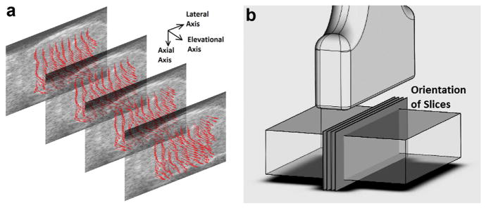
(a) Graphic rendering of the fiber orientation within four planes. These planes were spaced 0.203 mm apart and were the data points included in the non-linear curve fit. Fiber orientations are indicated by arrows. Note that all arrows are plotted with the same lengths, but some arrows appear shorter because of their orientation. These arrows are plotted at one-eighth of the actual data resolution. (b) Orientation of the four planes in (a) with respect to the ultrasound transducer and sample.
Three representative histologic images along with histology-quantified fiber orientations are provided in Figure 9a–c. These are taken from the outer (near epicardium), middle (myocardial) and inner (near endocardium) layers.
Fig. 9.

Images of Masson trichrome-stained rat left ventricular myocardium samples in the lateral-elevational plane. Three samples at different tissue depths are illustrated: Near the epicardium (a), in the middle myocardium layer (b) and near the endocardium (c). Fiber orientations were computed on the basis of these images using 2-D Fourier analysis and were plotted as solid lines at approximate locations where analysis using our ultrasound-biaxial method was performed. Bar = 100 μm. (d) Schematic of the orientation of these histology samples with respect to ultrasound-biaxial mechanical testing. (e) Plot of fiber orientation versus tissue depth (axial coordinates) near the central region of the sample, shown for two-thirds of the total thickness of the sample. Both data computed using histology (black line) and data computed using ultrasound-biaxial mechanical testing (gray lines) are illustrated. With the latter, each gray line corresponds to one of the four planes analyzed. The approximate outer (epicardium) and inner (endocardium) boundaries of the sample are indicated as dotted lines on the left and right edges of the plot.
Figure 9e illustrates the comparison between fiber orientations computed from the biaxial-ultrasound experiment with our curve-fitting algorithm and those quantified by histology. Fiber orientations were plotted versus axial coordinates (depth of sample). Data obtained from the two techniques were in satisfactory agreement. Generally, a gradual increase in the fiber angle of approximately 57° is observed from the outer layers to the inner layers over the half-thickness of the myocardium investigated.
DISCUSSION
We have introduced a new technique for mechanical testing of biological samples that combines 3-DUST with traditional biaxial mechanical testing. Our technique improves on the traditional testing techniques by using 3-D ultrasound for volumetric imaging instead of optical tracking, which allows only superficial tracking. Three-dimensional ultrasound speckle tracking combined with biaxial testing could provide the complete set of spatially varying strain tensors over entire 3-D volumes, thus providing more information than traditional mechanical testing.
The current implementation represents only one possible setup in which ultrasound elasticity imaging and mechanical testing can be combined. Ultrasound elasticity imaging can also be combined with other mechanical testing methods including vascular pressure–diameter and force–length mechanical testing (Gleason et al. 2007), three-point bending tests for heart valves (Gloeckner et al. 1999), pure shear tests for the liver (Gao et al. 2010) and simple uniaxial compression tests. These implementations may yield important new details, for example, spatially varying fiber orientation or spatially varying mechanical properties, which may help in investigations of 3-D vascular wall prestresses (Chuong and Fung 1986; Rachev and Greenwald 2003; Wang and Gleason 2010). Further, in many cases, biomaterial implants experience inhomogeneous tissue growth at different layers of the implant (Kalfa et al. 2010; Wei et al. 2006). The spatially varying tissue architecture and mechanical properties can be evaluated by 3-DUST combined with mechanical testing. Additionally, if in vivo stresses can be approximated (by using hoop stress theory or in vivo force measuring devices), the technique may even be translatable to in vivo evaluation of mechanical properties.
FEA of the non-linear curve-fitting algorithm
Finite-element analyses were performed for the first SEF (eqn 10) only, and the SEF parameters assumed in the simulations are provided in the last row of Table 1. Only tissue displacement and boundary stress data from the FEA were input into the non-linear curve-fitting algorithm, which was used to compute the SEF. For simulation cases with homogeneous fiber angle, the algorithm-computed SEF matched the original SEF very well (Table 1), indicating that the algorithm could retrieve the SEF. Further, one set of loading conditions was sufficient for the SEF computation.
From the FEA, we found that, for inhomogeneous fiber angle cases, optimal use of the non-linear curve-fitting algorithm was achieved by inputting data from two loading conditions, which is equivalent to testing the sample twice under different loading patterns, and using measurements from both tests in the same SEF computation. This approach was found to enhance both accuracy (Table 2) and convergence, because from our experience, convergence failure sometimes results if only one loading condition is entered into the nonlinear curve-fitting computation. This was also observed during computation with experimental data. When convergence failure occurs, usually one SEF parameter would continually trade magnitude with another, and this may continue even when the two parameters are orders of magnitude apart. Humphrey et al. (1990c) reported difficulty in convergence while using the first SEF (eqn 10), as well. We believe that our observation of non-convergence indicates the non-uniqueness of solutions for model fitting using single-loading-condition test data. This non-uniqueness of solutions in model fitting of mechanical testing is explained in detail by Ogden et al (2004), who reported that when test data from two loading conditions are concurrently used for model fitting, good overall fits are obtained with reasonably low relative errors, but not so for data from only one loading condition. This corroborates our observations, and we thus adopted the dual-loading protocol for all experiments. However, the non-uniqueness problem requires further in-depth studies for comprehensive characterization and understanding, so as to develop a formal treatment. Future investigation is thus warranted.
Figure 4 illustrated satisfactory accuracy of the algorithm-computed fiber orientations for inhomogeneous fiber cases as well. From the first casein Figure 4a, we noted that for fiber angles near directions of loading (0 and 90°), errors were consistently higher, but this was found to be a characteristic of the SEF used: When we switched from the first SEF (eqn 10) to the second SEF (eqn 11), the problem ceased. In the second fiber pattern case (Fig. 4b), higher errors were encountered, most likely because the nonuniformity in cross-sectional stresses increased, which conflicted with our algorithm’s assumption of uniform cross-sectional stress.
Ultrasound mechanical testing of rat left ventricle
The experimental biaxial testing was performed under quasi-static conditions rather than in real time because the high-frequency ultrasound transducer used was a 1-D linear array for cross-sectional 2-D imaging. Real-time 3-D scanning could not be achieved, and 3-D scans had to be achieved by translating the transducer in the elevational axis with a linear actuator, acquiring a stack of 2-D ultrasound images and undergoing 3-D reconstruction. It took a few seconds to acquire each 3-D volume image, during which the sample needs to be held stationary, thus requiring the quasi-static testing protocol. This method was adopted because high-frequency 2-D array transducers for 3-D volume imaging are not readily available yet. However, when they are available, our technique can be improved and adapted for real-time dynamic testing.
Because the quasi-static testing protocol was adopted, we implemented strategies to counter viscoelastic stress relaxation and then evaluated whether stress relaxation posed a problem to our measurements. To counter stress relaxation effects, between consecutive stretching cycles of the sample, the sample was relaxed to the stretch-free state and maintained under this condition for 6 s for recovery. In Figure 5a, we compared the force-displacement curve of the quasi-static protocol (illustrated by the black dots, which represent the conditions under which ultrasound imaging were performed amid the multiple cycles of stretching) with the force-displacement curve of a fully dynamic stretching cycle (represented by the black line, which is the stretching cycle of the last preconditioning cycle). Figure 5a illustrates that the black dots (quasi-static protocol) were close to the loading arm of the black line (fully dynamic protocol), indicating that our quasi-static protocol could approximate a fully dynamic protocol using our strategy described above.
Figure 5c and d qualitatively illustrates that a sufficiently high density of speckles could be imaged and that piecing multiple image slices together could still produce a good continuum of speckles in the elevational direction, enabling high-fidelity correlation for 3-DUST (Fig. 6a).
From the non-linear curve-fitting computation results, we could obtain satisfactory matches between stresses computed from the algorithm and those computed from experimental measurements, as illustrated in Figure 7a, for both loading conditions (two different mechanical tests on the same sample) that the sample underwent. With the first SEF (eqn 10), the match in loading condition 2 was not as good. We find that this can be resolved by using the second SEF (eqn 11), as illustrated in Figure 7b. Figure 7a and b further illustrate that there were significant spatial variations in stresses around its mean value. This could be due to realistic spatial variation in stresses, or errors stemming from spatial variation of material stiffness, or a combination of the two.
The recovered SEF coefficients, as outlined in Table 4, were of the same order of magnitude as those reported by Humphrey and colleagues (Humphrey and Yin 1987; Humphrey et al. 1990b, 1990c), who originally designed these SEFs. It should be noted that we report values in kilopascals instead of grams per square centimeter, as Humphrey et al. did. The comparison of our SEF values with those of Humphrey et al., however, should be interpreted with caution, because the samples are from different animals (canine vs. rat), and the testing protocols are different. We have nonetheless chosen to compare our results with this previous work because, to the best of our knowledge, there is no report of small animal biaxial myocardial experimental testing using these specific forms of SEFs.
Possibility of computing fiber orientation from 3-DUST mechanical testing
In the current implementation, during computation of the SEF parameters with the non-linear curve-fitting algorithm, spatially varying fiber orientations were also computed. We investigated whether this computed fiber orientation approximated the true fiber orientation of the test sample by histologically analyzing the same sample that underwent mechanical testing. Our preliminary results indicated that combining 3-DUST with mechanical testing may be a good method for concurrently retrieving both mechanical properties and spatially varying fiber orientations. However, further work is required to fully validate this technique for estimating tissue fiber orientation.
From histology and from ultrasound-biaxial experiments, it was found that the variation in fiber orientation from the outer layers to the inner layers over an approximately 2-mm thickness of myocardium, or about two-thirds of the full thickness, was about 57° (Fig. 9e), which translates to 86° over the entire sample thickness. This result was in good agreement with fiber orientations computed through histology when plotted as a function of axial coordinates. The variation of 86° over the entire thickness of the myocardium was close to but slightly lower than values from other groups (Chen et al. 2003; Hsu et al. 1998; Reese et al. 1995; Tezuka 1975), who reported variations of approximately 100°–150° over the entire thickness of the myocardium in rat, canine and human hearts.
Limitations
In our current implementation combining ultrasound and biaxial mechanical testing, the fiber orientation was assumed to be purely in the lateral-axial plane (in line with the biaxial testing), with no axial component. This idealization was adopted to simplify the non-linear curve-fitting computation while we establish the foundation for this new technique. Future work describing fiber orientation with two angle coefficients to fully account for 3-D fiber orientation can be implemented with no complication, if the non-linear curve-fitting computation is carried out with more efficient programming language to enhance the computation capacity.
A second and major limitation to our work is the assumption of uniform stresses within a cross section in the elevational and lateral directions, and the assumption that stress is merely force measured by the biaxial actuators divided by the cross-sectional area measured by ultrasound. Our assumption was made because there is no known method of directly measuring internal stresses in the sample. In a non-homogeneous sample such as the myocardium, spatially varying fiber orientations will naturally cause stress non-uniformity as the sample is being stretched. Our present methodology cannot cater to this non-uniformity and will thus lead to errors.
CONCLUSIONS
The feasibility of using 3-D ultrasound speckle tracking in biaxial mechanical testing in silico and ex vivo was described. The method relied on a non-linear curve-fitting algorithm to compute the strain energy function using only tissue displacement and boundary stress information. This algorithm was tested on synthetic ultrasound data from finite-element simulations and was found to be accurate. Preliminary ex vivo results using excised rat cardiac wall tissue revealed that the combination of 3-D ultrasound speckle tracking with biaxial mechanical testing may be able to accurately estimate spatially varying fiber orientation in addition to the mechanical properties of the biological tissue samples.
Parameters were first computed for every quasi-static step and then averaged over all quasi-static steps before being reported. Our investigations suggested that the goodness of fit obtained from fitting the material model to ultrasound-biaxial experimental measurements is dependent on the model assumed.
Acknowledgments
This study was supported in parts by GRO-Samsung (Principal Investigator [PI]: K.K.), NIH 1 R21 EB013353-01 (PI: K.K.), NIH 1 S10 RR027383-01 (PI: K.K.), AHA Beginning Grant-in-Aid 10 BGI A3790022 (PI: M.S.) and the Pittsburgh Foundation M2010-0052 (PI: M.S.). The authors thank Daniela Valdez-Jasso, Andrea Sebastiani and Sunaina Rustagi for assisting with experiments and helpful discussions.
Footnotes
All authors have no conflicts of interest to declare.
References
- Arts T, Costa KD, Covell JW, McCulloch AD. Relating myocardial laminar architecture to shear strain and muscle fiber orientation. Am J Physiol Heart Circ Physiol. 2001;280:H2222–H2229. doi: 10.1152/ajpheart.2001.280.5.H2222. [DOI] [PubMed] [Google Scholar]
- Chen J, Song SK, Liu W, McLean M, Allen JS, Tan J, Wickline SA, Yu X. Remodeling of cardiac fiber structure after infarction in rats quantified with diffusion tensor MRI. Am J Physiol Heart Circ Physiol. 2003;285:H946–H954. doi: 10.1152/ajpheart.00889.2002. [DOI] [PubMed] [Google Scholar]
- Chen X, Xie H, Erkamp R, Kim K, Jia C, Rubin JM, O’Donnell M. 3-D correlation-based speckle tracking. Ultrason Imaging. 2005;27:21–36. doi: 10.1177/016173460502700102. [DOI] [PubMed] [Google Scholar]
- Chuong CJ, Fung YC. On residual stresses in arteries. J Biomech Eng. 1986;108:189–192. doi: 10.1115/1.3138600. [DOI] [PubMed] [Google Scholar]
- Gao Z, Lister K, Desai JP. Constitutive modeling of liver tissue: Experiment and theory. Ann Biomed Eng. 2010;38:505–516. doi: 10.1007/s10439-009-9812-0. [DOI] [PMC free article] [PubMed] [Google Scholar]
- Glagov S, Vito R, Giddens DP, Zarins CK. Micro-architecture and composition of artery walls: Relationship to location, diameter and the distribution of mechanical stress. J Hypertens Suppl. 1992;10:S101–S104. [PubMed] [Google Scholar]
- Gleason RL, Wilson E, Humphrey JD. Biaxial biomechanical adaptations of mouse carotid arteries cultured at altered axial extension. J Biomech. 2007;40:766–776. doi: 10.1016/j.jbiomech.2006.03.018. [DOI] [PubMed] [Google Scholar]
- Gloeckner DC, Billiar KL, Sacks MS. Effects of mechanical fatigue on the bending properties of the porcine bioprosthetic heart valve. ASAIO J. 1999;45:59–63. doi: 10.1097/00002480-199901000-00014. [DOI] [PubMed] [Google Scholar]
- Holzapfel GA, Ogden RW. Constitutive modelling of passive myocardium: A structurally based framework for material characterization. Philos Trans A Math Phys Eng Sci. 2009;367:3445–3475. doi: 10.1098/rsta.2009.0091. [DOI] [PubMed] [Google Scholar]
- Hsu EW, Muzikant AL, Matulevicius SA, Penland RC, Henriquez CS. Magnetic resonance myocardial fiber-orientation mapping with direct histologic correlation. Am J Physiol. 1998;274:H1627–H1634. doi: 10.1152/ajpheart.1998.274.5.H1627. [DOI] [PubMed] [Google Scholar]
- Humphrey JD. Cardiovascular solid mechanics: Cells, tissues, and organs. Berlin/Heidelberg: Springer; 2002. [Google Scholar]
- Humphrey J, Strumpf R, Yin F. Biaxial mechanical behavior of excised ventricular epicardium. Am J Physiol. 1990a;259:H101–H108. doi: 10.1152/ajpheart.1990.259.1.H101. [DOI] [PubMed] [Google Scholar]
- Humphrey JD, Strumpf RK, Yin FC. Determination of a constitutive relation for passive myocardium: I. A new functional form. J Biomech Eng. 1990b;112:333–339. doi: 10.1115/1.2891193. [DOI] [PubMed] [Google Scholar]
- Humphrey JD, Strumpf RK, Yin FC. Determination of a constitutive relation for passive myocardium: II. Parameter estimation. J Biomech Eng. 1990c;112:340–346. doi: 10.1115/1.2891194. [DOI] [PubMed] [Google Scholar]
- Humphrey JD, Yin FC. On constitutive relations and finite deformations of passive cardiac tissue: I. A pseudostrain-energy function. J Biomech Eng. 1987;109:298–304. doi: 10.1115/1.3138684. [DOI] [PubMed] [Google Scholar]
- Kalfa D, Bel A, Chen-Tournoux A, Della Martina A, Rochereau P, Coz C, Bellamy V, Bensalah M, Vanneaux V, Lecourt S, Mousseaux E, Bruneval P, Larghero J, Menasche P. A polydioxanone electrospun valved patch to replace the right ventricular outflow tract in a growing lamb model. Biomaterials. 2010;31:4056–4063. doi: 10.1016/j.biomaterials.2010.01.135. [DOI] [PubMed] [Google Scholar]
- Konofagou E, Ophir J. A new elastographic method for estimation and imaging of lateral displacements, lateral strains, corrected axial strains and Poisson’s ratios in tissues. Ultrasound Med Biol. 1998;24:1183–1199. doi: 10.1016/s0301-5629(98)00109-4. [DOI] [PubMed] [Google Scholar]
- Lubinski MA, Emelianov SY, O’Donnell M. Speckle tracking methods for ultrasonic elasticity imaging using short-time correlation. IEEE Trans Ultrason Ferroelectr Freq Control. 1999;46:82–96. doi: 10.1109/58.741427. [DOI] [PubMed] [Google Scholar]
- Meunier J. Tissue motion assessment from 3-D echographic speckle tracking. Phys Med Biol. 1998;43:1241–1254. doi: 10.1088/0031-9155/43/5/014. [DOI] [PubMed] [Google Scholar]
- More JJ, Sorensen DC. Computing a trust region step. Siam J Sci Stat Comp. 1983;4:553–572. [Google Scholar]
- O’Donnell M, Skovoroda AR, Shapo BM, Emelianov SY. Internal displacement and strain imaging using ultrasonic speckle tracking. IEEE Trans Ultrason Ferroelectr Freq Control. 1994;41:314–325. [Google Scholar]
- Ogden R, Saccomandi G, Sgura I. Fitting hyperelastic models to experimental data. Comput Mech. 2004;34:484–502. [Google Scholar]
- Ophir J, Cespedes I, Ponnekanti H, Yazdi Y, Li X. Elastography: A quantitative method for imaging the elasticity of biological tissues. Ultrason Imaging. 1991;13:111–134. doi: 10.1177/016173469101300201. [DOI] [PubMed] [Google Scholar]
- Rachev A, Greenwald SE. Residual strains in conduit arteries. J Biomech. 2003;36:661–670. doi: 10.1016/s0021-9290(02)00444-x. [DOI] [PubMed] [Google Scholar]
- Reese TG, Weisskoff RM, Smith RN, Rosen BR, Dinsmore RE, Wedeen VJ. Imaging myocardial fiber architecture in vivo with magnetic resonance. Magn Reson Med. 1995;34:786–791. doi: 10.1002/mrm.1910340603. [DOI] [PubMed] [Google Scholar]
- Sacks MS. Biaxial mechanical evaluation of planar biological materials. J Elasticity. 2000;61:199–246. [Google Scholar]
- Scollan DF, Holmes A, Zhang J, Winslow RL. Reconstruction of cardiac ventricular geometry and fiber orientation using magnetic resonance imaging. Ann Biomed Eng. 2000;28:934–944. doi: 10.1114/1.1312188. [DOI] [PMC free article] [PubMed] [Google Scholar]
- Skovoroda AR, Emelianov SY, Lubinski MA, Sarvazyan AP, O’Donnell M. Theoretical analysis and verification of ultrasound displacement and strain imaging. IEEE Trans Ultrason Ferroelectr Freq Control. 1994;41:302–313. [Google Scholar]
- Stuber M, Scheidegger MB, Fischer SE, Nagel E, Steinemann F, Hess OM, Boesiger P. Alterations in the local myocardial motion pattern in patients suffering from pressure overload due to aortic stenosis. Circulation. 1999;100:361–368. doi: 10.1161/01.cir.100.4.361. [DOI] [PubMed] [Google Scholar]
- Tezuka F. Muscle fiber orientation in normal and hypertrophied hearts. Tohoku J Exp Med. 1975;117:289–297. doi: 10.1620/tjem.117.289. [DOI] [PubMed] [Google Scholar]
- Urheim S, Edvardsen T, Torp H, Angelsen B, Smiseth OA. Myocardial strain by Doppler echocardiography: Validation of a new method to quantify regional myocardial function. Circulation. 2000;102:1158–1164. doi: 10.1161/01.cir.102.10.1158. [DOI] [PubMed] [Google Scholar]
- Wang R, Gleason RL., Jr A mechanical analysis of conduit arteries accounting for longitudinal residual strains. Ann Biomed Eng. 2010;38:1377–1387. doi: 10.1007/s10439-010-9916-6. [DOI] [PMC free article] [PubMed] [Google Scholar]
- Wei HJ, Chen SC, Chang Y, Hwang SM, Lin WW, Lai PH, Chiang HK, Hsu LF, Yang HH, Sung HW. Porous acellular bovine pericardia seeded with mesenchymal stem cells as a patch to repair a myocardial defect in a syngeneic rat model. Biomaterials. 2006;27:5409–5419. doi: 10.1016/j.biomaterials.2006.06.022. [DOI] [PubMed] [Google Scholar]