Computed inverse MRI for magnetic susceptibility map reconstruction

Abstract

Objective

This paper reports on a computed inverse magnetic resonance imaging (CIMRI) model for reconstructing the magnetic susceptibility source from MRI data using a two-step computational approach.

Methods

The forward T2*-weighted MRI (T2*MRI) process is decomposed into two steps: 1) from magnetic susceptibility source to fieldmap establishment via magnetization in a main field, and 2) from fieldmap to MR image formation by intravoxel dephasing average. The proposed CIMRI model includes two inverse steps to reverse the T2*MRI procedure: fieldmap calculation from MR phase image and susceptibility source calculation from the fieldmap. The inverse step from fieldmap to susceptibility map is a 3D ill-posed deconvolution problem, which can be solved by three kinds of approaches: Tikhonov-regularized matrix inverse, inverse filtering with a truncated filter, and total variation (TV) iteration. By numerical simulation, we validate the CIMRI model by comparing the reconstructed susceptibility maps for a predefined susceptibility source.

Results

Numerical simulations of CIMRI show that the split Bregman TV iteration solver can reconstruct the susceptibility map from a MR phase image with high fidelity (spatial correlation≈0.99). The split Bregman TV iteration solver includes noise reduction, edge preservation, and image energy conservation. For applications to brain susceptibility reconstruction, it is important to calibrate the TV iteration program by selecting suitable values of the regularization parameter.

Conclusions

The proposed CIMRI model can reconstruct the magnetic susceptibility source of T2*MRI by two computational steps: calculating the fieldmap from the phase image and reconstructing the susceptibility map from the fieldmap. The crux of CIMRI lies in an ill-posed 3D deconvolution problem, which can be effectively solved by the split Bregman TV iteration algorithm.

1. Introduction

A medical imaging system is sensitive to specific physical properties ¹, such as the computed tomography (CT) to x-ray attenuation coefficient (or largely the material density), optical imaging to photonic absorption/reflection/scattering, positron emission tomography (PET) to radionuclide trace distribution, and magnetic resonance imaging (MRI) to magnetic field perturbation. By adjusting multiple parameters, an MRI system may be tuned to favor a specific physical property to produce a specific image contrast such as² T1, T2, T2*, spin density, etc. In this paper we focus on T2*-weighted MRI (denoted by T2*MRI) which measures the transverse magnetization relaxation due to spin precession dephasing in an inhomogeneous field. Since the inhomogeneous fieldmap is usually caused by a source of inhomogeneous susceptibility distribution via magnetization in a main field, the inhomogeneous susceptibility map (SM) is considered as the underlying source of T2*MRI. In order to estimate this underlying source, we suggest to reconstruct it from the T*MRI data through an inverse process. There is growing interest in susceptibility mapping^3-8. In this paper, we describe the T2*MRI procedure and propose a computed inverse MRI (CIMRI) model for reconstructing the SM source from a MR phase image by a two-step computational inverse mapping.

The fieldmap is established from a SM via magnetization in a main field, which can be described by a 3D convolution transform. The expression of the magnetization mechanism as a 3D convolution allows us to estimate the SM source by solving a 3D deconvolution problem. A T2*MRI experiment produces a complex-valued image from an average of intravoxel dephasing^2,9. Due to the involvement of spin precession signals (in the form of a complex exponential) and operations for complex modulo and phase arguments, the T2*MRI procedure is an overall nonlinear mapping: from a 3D SM to a 3D MR magnitude image and a 3D MR phase image. There have been a number of previous studies on computing susceptibility maps. However the early SM reconstruction efforts on SM reconstruction were only concerned with simple regular geometry (most commonly for spheres and cylinders)^10-12. In order to accommodate arbitrary susceptibility distributions, we propose a CIMRI model that computationally reconstructs the SM source from a MR phase image acquired by T2*MRI.

Recent SM computation efforts can be classified into three categories: (i) Tikhonovregularized matrix inverse, (ii) inverse filtering, and (iii) iterative optimization. In particular, the matrix inverse technique utilizes well-established matrix algebra, especially the Tikhonov regularization techniques for ill-posed matrix inverse^3,4. However this approach requires one to convert a 3D convolution into a 2D matrix format ⁴, which usually leads to a very large 2D matrix that makes inverse calculation difficult (See Appendix A). Another approach to deal with the 3D deconvolution problem is based on filtering theory. In the Fourier domain, a 3D deconvolution is converted into a 3D inverse filtering (3D element-wise array division). Since there is a zerosurface on the 3D filter (the Fourier transform of the convolution kernel), the inverse filtering is confronted with a divide-by-zero problem. One typical solution is to regularize the solution by using a truncated inverse filter^9-15. The filter truncation is a nonlinear operation, which may change the image energy and cause artifacts.

Recently, image restoration has been well solved by using total variation (TV) regularization strategies^16-20. The TV regularization and Bregman iteration technique have been used for MR image reconstruction from multichannel parallel imaging ⁵ (in the framework of Fourier transformation in a k-space). It has been shown that TV regularization is an excellent technique for 2D image restoration. In this work we will generalize the TV-based 2D image restoration strategy to accommodate our 3D SM reconstruction goal.

2. Theory and algorithms

An overview of T2*MRI brain imaging is shown in Fig. 1, consisting of two modules: the Source Magnetism module (in the upper dashed box) that offers a SM (as the source for T2*MRI) like a brain physiological state, and the MRI Technology module (in the lower dashed box) that produces a complex-valued image for the SM source. In the MRI technology module, the forward T*MRI procedure consists of two steps: the fieldmap establishment from a SM source via susceptibility magnetization, and the complex image formation from the fieldmap via intravoxel dephasing (indicated by the two downward arrows). Correspondingly, the CIMRI consists of two inverse computation steps: fieldmap calculation and SM calculation (indicated by the two upward arrows, and highlighted in the circle). For brain imaging, the SM may consist of both functional and structural contributions (in particular, the static non-heme iron deposit and dynamic heme iron perturbation). For tissue and organ imaging, the SM source represents the non-heme iron deposit in anatomy, and in this sense the SM reconstruction by CIMRI serves as an iron imaging modality.

Fig. 1.

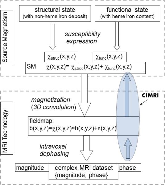
Overall diagrams for the forward T2*MRI and the computed inverse MRI (CIMRI). In the upper dashed box, the ‘Source Magnetism’ module provides a magnetic susceptibility map (SM) expression for an imaging target (illustrated with a brain physiological state for brain imaging). In the lower dashed box, the “MRI Technology” module takes the SM as the input source and produces a complex-valued output dataset. Reversely, diagrammed by two upward arrows, the CIMRI reconstructs the SM source from the phase image in the T2*MRI output.

2.1 Magnetic susceptibility source formulation

As diagramed in Fig. 1, we assume that the total magnetic susceptibility source of T2*MRI is given by

$${\chi }_{total}(x,y,z)={\chi }_{struc}(x,y,z)+{\chi }_{func}(x,y,z)$$ (1)

where χ_struc(x,y,z) denotes the susceptibility distribution due to the structural biomagnetism, and χ_func(x,y,z) a snapshot of a dynamic susceptibility perturbation (at an event time) due to a functional activity. It is noted that we can represent a dynamic susceptibility process by incorporating the time-dependence as χ_func(x,y,z,t) and χ_total(x,y,z,t). In the following we focus on a 3D SM reconstruction from a MR phase image captured at a snapshot by T2*MRI (with an echo time T_E).

The contribution to χ_struc(x,y,z) is mainly due to the iron deposit in tissues and organs (in addition to minor contributions from non-iron contents). For brain imaging, χ_struc(x,y,z) is mainly attributed to non-heme iron deposition in brain parenchyma and vascular blood. In the brain, χ_struc(x,y,z) may assume a range of susceptibility values: from negative diamagnetic (such as water and blood) to positive paramagnetic values (such as ferritin and hemosiderin).

The contribution to χ_func(x,y,z) is attributed to a complicated neuron-modulated vascular blood magnetism perturbation. Let NAB(x,y,z) denote a local neuroactivity (NAB: neuroactive blob), which stimulates a blob-like region inside a cerebral cortical field of view (FOV). We assume a spatial modulation model for the neuron-induced intravascular magnetism perturbation, which gives rise to a brain functional state as

$$\begin{array}{cc}\hfill & {\chi }_{total}(x,y,z)={\chi }_{base}(x,y,z)+{\chi }_{BOLD}(x,y,z)\text{with}\hfill \\ \hfill & {\chi }_{BOLD}(x,y,z)=({\chi }_{deoxy}-{\chi }_{oxy})(1-Y)\cdot Hct\cdot V(x,y,z)\cdot NAB(x,y,z)\hfill \end{array}$$ (2)

where V(x,y,z) denotes the vasculature-laden brain FOV, χ_oxy and χ_deoxy denote blood oxygenated and deoxygenated magnetic susceptibilities, Y the blood oxygenation level, Hct the blood hematocrit. In Eq.(2), the total brain SM at a snapshot is decomposed into a static baseline state (χ_base) and a dynamic BOLD perturbation state (χ_BOLD). Specifically, χ_base accounts for the susceptibility contributions from static brain structure, blood plasma, and fully oxygenated blood, and χ_BOLD only accounts for the change in the heme-iron magnetism due to a BOLD activity. It has been experimentally determined that χ_deoxy -χ_oxy =0.27×4π×10⁻⁶ (SI unit) ²², which implies that the BOLD effect is a positive paramagnetic perturbation (under the spatial neuronal modulation).

2.2 MR signal and image acquisition

2.2.1 Fieldmap disturbance due to SM magnetization

When an entity such as a brain is placed in a main magnetic field B₀, it undergoes a material-and-field magnetization interationn and imposes an inhomogeneous field distribution over B₀. Let χ(x,y,z) denote the SM of the material susceptibility, M(x,y,z) the magnetization vector density, then the linear material magnetization in B₀ is described by ²³

$$\begin{array}{cc}\hfill {\mu }_0\cdot \mathbf{M}\left(\mathbf{r}\right)=& \chi \left(\mathbf{r}\right)\cdot {\mathbf{B}}_0,\hfill \\ \hfill \text{and}{\mu }_0\cdot M_z\left(\mathbf{r}\right)=& \chi \left(\mathbf{r}\right)\cdot B_0\text{for}{\mathbf{B}}_0={\mathit{B}}_0\widehat{z}\hfill \end{array}$$ (3)

where r=(x,y,z), and we are concerned with M_z(r) (the z-component of M(r)) that is parallel to B₀. It is known that the magnetic field disturbance, denoted by B(r), due to the source of M(r), is given by ⁶

$$\begin{array}{cc}\hfill \mathbf{B}\left(\mathbf{r}\right)=& \frac{{\mu }_0}{4\pi }\int \int \int \nabla \times \left[\mathbf{M}\left({\mathbf{r}}^{\prime }\right)\times \frac{(\mathbf{r}-{\mathbf{r}}^{\prime })}{{\mid \mathbf{r}-{\mathbf{r}}^{\prime }\mid }^3}\right]d^3{\mathbf{r}}^{\prime }\left(\text{exact}\right)\hfill \\ \hfill \approx & \frac{{\mu }_0}{4\pi }\int \int \int \left[\frac{3\mathbf{M}\left({\mathbf{r}}^{\prime }\right)\cdot (\mathbf{r}-{\mathbf{r}}^{\prime })}{{\mid \mathbf{r}-{\mathbf{r}}^{\prime }\mid }^5}(\mathbf{r}-{\mathbf{r}}^{\prime })-\frac{\mathbf{M}\left({\mathbf{r}}^{\prime }\right)}{{\mid \mathbf{r}-{\mathbf{r}}^{\prime }\mid }^3}\right]d^3{\mathbf{r}}^{\prime }\left(\text{point dipole model}\right)\hfill \end{array}$$ (4)

Under linear magnetization in B₀ (in Eq. (3)) and point magnetic dipole model (in Eq. (4)), the fieldmap of B_z(r) (z-component of B(r)) is given by ²⁴

$$\begin{array}{cc}\hfill & B_z\left(\mathbf{r}\right)=B_0\cdot \chi \left(\mathbf{r}\right)\ast h\left(\mathbf{r}\right)\hfill \\ \hfill & \text{with}h\left(\mathbf{r}\right)=\frac{1}{4\pi }\frac{3z^2-{\mathbf{r}}^2}{{\mid \mathbf{r}\mid }^5}\hfill \end{array}$$ (5)

where * denotes a 3D convolution, h(r) is a convolution kernel (or Green's function). The 3D distribution of B_z(r) is a fieldmap, denoted by b(r) henceforth. In practice, the fieldmap measurement involves noise. With an additive Gaussian noise, denoted by ε(r), we describe the fieldmap establishment from material magnetization by a general 3D convolution formula

$$b\left(\mathbf{r}\right)=B_0\chi \left(\mathbf{r}\right)\ast h\left(\mathbf{r}\right)+\epsilon \left(\mathbf{r}\right)$$ (6)

which shows that the task of finding the magnetic susceptibility from a fieldmap is to solve an inverse problem of 3D convolution in presence of noise.

Considering Eq.(6) as a 3D imaging system, we can describe its imaging performance through the characteristics of its 3D kernel h(r). It can be shown that

$$\begin{array}{cc}\hfill & \{\begin{array}{cc}{\int \int \int }_{(\mathrm{x},\mathrm{y},\mathrm{z})}h(x,y,z)dxdydz=\mathrm{H}(0,0,0)\hfill & (\text{filer DC}<1)\hfill \\ {\int \int \int }_{(\mathrm{x},\mathrm{y},\mathrm{z})}\mid h(x,y,z)\mid dxdydz>>\mathrm{H}(0,0,0)\hfill & \left(\text{dipolar-valued kernel}\right)\hfill \end{array}\phantom{\}}\hfill \\ \hfill & \text{with}H(k_x,k_y,k_z)=FT\left\{h(x,y,z)\right\}=\frac{1}{3}-\frac{k_z^2}{(k_x^2+k_y^2+k_z^2)}\hfill \end{array}$$ (7)

where FT denotes Fourier transform. It is noted that there is an uncertainty for H(0,0,0). Usually the DC term of the 3D filter H(k_x,k_y,k_y) assumes H(0,0,0) =1/3 (when 0/0=0 is used in Eq.(7)). From the viewpoint of image processing ⁷, the local spatial integral property of h(x,y,z) in Eq. (7) plays a 3D textural enhancer. In Fig.2 (a) and (b), we visualize the 3D kernel by 3D isosurfaces and a 2D slice, respectively. The zerosurface at the 2D kernel slice manifests as two crossed edges in Fig. 2(c), which allows us to interpret the convolution in the sense of textural enhancement. A texture template can serve as an edge enhancement due to textural edges, but is not optimal for edge detection due to textural edge irregularity (as the crossed edges in Fig. 2(c)).

Fig. 2.

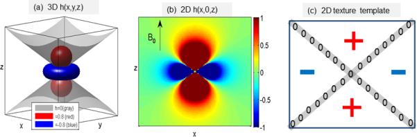
(a) Visualization of the 3D convolution kernel h(x,y,z) with three isosurfaces at isovalues of {0, 0.8, -0.8}; (b) the 2D quadrupole pattern at a longitudinal plane at h(x,0,z); (c) a digital texture template with two crossed edges (corresponding the conic zerosurface in (b)).

In what follows is a summary of the characteristics of the 3D kernel h(x,y,z):

• 1)It is of 3D spread distribution (in a decay ~1/r³, see h(r) definition in Eq. (5)), which explains the non-local property of the fieldmap and MR phase image.
• 2)It is a 3D bipolar-valued kernel that manifests a 3D texture enhancer as understandable from Eq.(7) and Fig. 2(b) and (c). Therefore, it is not surprising that the phase image appears noisy.
• 3)It bears a 3D conic zerosurface for h(x,y,z)=0 (see Fig. 2(a) and (c)); correspondingly there is 3D zerosurface for H(k)=0 as well. As a result, either the deconvolution or the inverse filtering will encounter an ill-posed problem.
• 4)It is anisotropic, which explains the vascular orientation dependence of fieldmap and MR image. In particular, if a vessel poses at the magic angle (54°) with respect to B₀, it makes no contribution to the fieldmap.
• 5)It is of radial symmetry about the origin (that is h(x,y,z)=h(-x,-y,-z)) and revolution symmetry about z-axis (that is h(x,y,z)=h(y,x,z)) (see Fig. 2(a)). However, there is no symmetry between longitudinal (along z-axis) and transversal direction (along x- or y-axis), that is, h(x, y, z) ≠ h(x, z, y) and h(x, y, z) ≠ h(z, y, z), which accounts for the anisotropy.

Overall, the 3D convolution kernel in Fig. 2 is a unusual integral kernel because of its bipolar-valued multilobes, anisotropic spreading, and 3D zerosurface embedment (usually, an image convolution kernel assumes a point-spread blur or a motion blur, which is of nonnegative distribution). However, the 3D convolution in Eq. (6) is a linear transformation that is characteristic of high dimension and a nonempty null space (matrix singularity).

2.2.2 Intravoxel dephasing signal and image formation

The voxel signal of T2*MRI is formed by intravoxel spin precession dephasing mechanism^3,26. Let Ω(x,y,z) denote the voxel at (x,y,z) in FOV, and |Ω| the voxel size, then the complex-valued voxel signal generated at echo time T_E is given by (in static dephasing regime)

$$C(x,y,z,T_E)=\frac{1}{\mid \Omega \mid }\sum _{(x^{\prime },y^{\prime },z^{\prime })\in \Omega (x,y,z)}\exp [-i\gamma b(x^{\prime },y^{\prime },z^{\prime })T_E]$$ (8)

where γ proton gyromagnetic ratio (=267.5×10⁶ rad/T), b(x,y,z) the inhomogeneous fieldmap over the FOV. The multivoxel image of T2*MRI is conceptually formed by a spatial tessellation of the voxel signals (In practice, the MR image is reconstructed from a k-space by Fourier transform). As a result, the output of T2*MRI is a complex-valued 3D multivoxel image as expressed in polar coordinate format by

$$C(x,y,z;T_E)=A(x,y,z;T_E)\exp [-iP(x,y,z;T_E)]$$ (9)

where the T_E is explicitly parameterized to show the dependence of gradient echo time. Note that the magnitude and phase calculation from a complex number is a nonlinear operation.

2.3 Computed inverse MRI

2.3.1 Fieldmap calculation from MR phase map

For the voxel signal phase, we may relate it the intravoxel averaged field value by the following approximation

$$P(x,y,z;T_E)=\angle C(x,y,z;T_E)-\angle C(x,y,z;T_E)\approx \gamma \cdot T_E\cdot b(x,y,z)$$ (10)

Therefore, we obtain that the multivoxel fieldmap by

$$b(x,y,z)=\frac{P(x,y,z;T_E)}{\gamma T_E}$$ (11)

Note that the linear relationship between phase image and fieldmap in Eq. (11) is only valid for the small angle regime⁸, where the phase angle P is so small such that exp(iP)≈1+iP and that the phase angle is far from wrapped (|P|<<π). When phase image are wrapped, the fieldmap may be obtained by a T_E-offset technique or by a phase-unwrapping technique. In this paper, we simplify the fieldmap calculation from MR phase image by Eq. (11) without involving the phase wrapping problems.

2.3.2 SM calculation from fieldmap

As seen in Fig. 1, the fieldmap is not the destination of CIMRI; it is just an expedient (or interim) for MRI technology to image the SM. Therefore, the determination of SM from fieldmap requires solving an inverse problem for Eq.(6), as represented by

$$\chi (x,y,z)=b(x,y,z){\ast }^{-1}h(x,y,z)$$ (12)

where *⁻¹ denotes deconvolution, and Eq. (12) represents deconvolving the fieldmap b(x,y,z) with the same kernel h(x,y,z) as used in Eq. (5). As aforementioned, the kernel bears a zerosurface, which poses an ill problem. In what follows, we tackle the 3D deconvolution problem in Eq.(12) using multiple approaches.

2.4 Solvers for inverse mapping from fieldmap to SM

2.4.1 Matrix inverse solver

Conceptually, if a process or transformation can be formulated into a matrix-vector multiplication, b=hx, (where x and b denote input and output vectors, and h the system matrix), we can readily solve the inverse process by matrix algebra by x=h⁻¹b as long as h is invertible. If h is singular (det(h)=0) or ill-posed (assuming a very large condition number, det(h)≈0 ), then h⁻¹ is not available. In such cases, a Tikhonov regularization or its variations is needed to solve the matrix inverse problem and to find an optimal solution, as typically given by x=(h^Th +αQ^TQ)⁻¹ h^Tb, where Q is a regularization matrix and α a regularization parameter ⁹. Therefore, in order to take advantage of the well-established matrix algebra and standard Tikhonov regularization, it is encouraged to formulate a minimization problem into a matrix format (in form of matrix-vector multiplication). The efforts on this kind of matrix solver can be found in ^3,4,10 .

Matrix inverse theory has been developed for 2D matrices and 1D vectors, but not for 3D matrices. (For example, there is no rule for 3D matrix multiplication or 3D matrix inverse). Therefore, we need to convert a discrete convolution into a matrix–vector multiplication format (see ⁹ ) if we wish to make use of the elegant matrix algebra. As presented in Appendix A, the convolution-to-matrix conversion may produce a 2D convolutional matrix (also called a system matrix) that is usually too big to find its inverse (in the sense of computation difficulty).

2.4.2 Filter truncation solver

The 3D convolution in Eq.(6) can be converted to a 3D multiplication in Fourier domain, that is

$$b\left(\mathbf{k}\right)=B_0\cdot {\chi }_{true}\left(\mathbf{k}\right)\cdot h\left(\mathbf{k}\right)+\epsilon \left(\mathbf{k}\right)\text{with}h\left(\mathbf{k}\right)=\frac{k_z^2}{{\mid \mathbf{k}\mid }^2}-\frac{1}{3}$$ (13)

where χ_true(k), b(k), ε(k) and h(k) denote the Fourier transforms of χ_true(r), b(r), ε(r) and h(r), respectively. Then an inverse filtering with a truncated filter is used to find the solution, denoted by χ*(k), as expressed by

$$\begin{array}{cc}\hfill & {\chi }^{\ast }\left(\mathbf{k}\right)=\frac{b\left(\mathbf{k}\right)}{B_0{h}_{trunc}\left(\mathbf{k}\right)}\hfill \\ \hfill & \text{with}{\mathrm{h}}_{\mathrm{trunc}}\left(\mathbf{k}\right)=\{\begin{array}{cc}{\epsilon }_0\cdot \mathrm{sgn}\left(h\left(\mathbf{k}\right)\right),\hfill & \mid h\left(\mathbf{k}\right)\mid <{\epsilon }_0\hfill \\ h\left(\mathbf{k}\right),\hfill & \text{otherwise}\hfill \end{array}\phantom{\}}\hfill \end{array}$$ (14)

where sgn(x) denotes a sign function (sgn(x)=1 for x> 0 and =-1 for x<0), and ε₀ is a small positive constant (e.g. 0.01). In the presence of noise (ε(k)≠0), the solution χ*(k) of the filter truncation solver (in Eq.(14)) is different from the truth χ_true(k) by

$${\chi }^{\ast }\left(\mathbf{k}\right)={\chi }_{true}\left(\mathbf{k}\right)\frac{h\left(\mathbf{k}\right)}{h_{trunc}\left(\mathbf{k}\right)}+\frac{\epsilon \left(\mathbf{k}\right)}{B_0{h}_{trunc}\left(\mathbf{k}\right)},\mid h\left(\mathbf{k}\right)\mid \le \mid h_{trunc}\left(\mathbf{k}\right)\mid \text{for}{\epsilon }_0>0$$ (15)

which shows that the filter truncation solver cannot exactly reconstruct the true χ map since |χ*(k)|≤|χ_true(k)|. Furthermore, it incurs a noise magnification by a factor of 1/(B₀h_trunc(k)) in Eq.(15). Since the truncated filter h_trunc(k) is bipolar-valued and anisotropic distributed in the Fourier domain, the noise magnification is spatial variant, that is,

$$\frac{1}{B_0{h}_{trunc}\left(\mathbf{k}\right)}=\{\begin{array}{c}1∕\left(B_0{\epsilon }_0\right),\mid h\left(\mathbf{k}\right)\mid <{\epsilon }_0\left(\text{at zerosurface}\right)\hfill \\ 3∕\left(2B_0\right),{\mathrm{k}}_{\mathrm{z}}^2∕{\mid \mathbf{k}\mid }^2=1\left(\text{along}{\mathrm{k}}_{\mathrm{z}}\text{axis}\right)\hfill \\ -3∕B_0,{\mathrm{k}}_{\mathrm{z}}^2∕{\mid \mathbf{k}\mid }^2=0(\text{at}{\mathrm{k}}_{\mathrm{x}}-{\mathrm{k}}_{\mathrm{y}}\text{plane})\hfill \end{array}\phantom{\}}$$ (16)

which indicates that the zerosurface of h(k) is always magnified (for B₀ε₀<1), the longitudinal direction is positively filtered, and the transverse direction is negatively filtered.

There have a plethora of reports on the filter truncation regularization for susceptibility mapping ^{3,4,6,7,30,31}, but none of them can solve the 3D deconvolution satisfactorily in the presence of noise. One challenge is to select an optimal ε₀ such that it only removes points at the zerosurface while conserving the image energy. Efforts at fine-tuning the truncation in Eq. (15) by smoothing the truncated zone (seeking a non-constant ε₀) and controlling the truncation zone thickness ³ may improve but not so profoundly.

2.4.3. TV-regularization solver

In recent years, the total variation (TV) iteration has been proven to be a very successful image restoration technique, in particular for 2D image restoration from a noisy and blurring image. In this subsection, we generalize the TV-regularized iteration algorithm to implement our 3D deconvolution problem in Eq.(12).

Mathematically, the TV norm for 3D susceptibility map χ(r) is defined as

$${\Vert \chi \Vert }_{TV}\equiv {\int }_{\Omega }\mid \nabla \chi \left(\mathbf{r}\right)\mid d\mathbf{r}={\int }_{\Omega }\sqrt{{\mid {\nabla }_x\left(\mathbf{r}\right)\mid }^2+{\mid {\nabla }_y\left(\mathbf{r}\right)\mid }^2+{\mid {\nabla }_z\left(\mathbf{r}\right)\mid }^2}d\mathbf{r}$$ (17)

Assuming a Gaussian noise model for ε(r), we can solve the 3D deconvolution in Eq.(12) by a TV-regularized unrestraint minimization problem ^11,12, as expressed by

$$\widehat{\chi }\left(\mathbf{r}\right)=\underset{\chi \in BV}{\min }{\Vert \chi \left(\mathbf{r}\right)\Vert }_{TV}+\frac{\lambda }{2}{\Vert B_{0}h\left(\mathbf{r}\right)\ast \chi \left(\mathbf{r}\right)-b\left(\mathbf{r}\right)\Vert }_2^2$$ (18)

where BV is a bounded variation function space, and λ is the Lagrange multiplier or the regularization parameter. The TV regularization lies in its searching over all possible distributions (χ∈BV) to find an optimal distribution $\widehat{\chi }$ such that it minimizes TV norm and the data fidelity error simultaneously.

It is known that Bregman iteration algorithm can facilitate convergence¹². We extend the split Bregman algorithm¹³ to solve the 3D minimization problem in Eq. (18) by a split Bregman iteration. In appendix B, we present details about a 3-subproblem split Bregman iteration algorithm that splits the 3D minimization problem into three iteration subproblems with respect to interim variables {‘d’, ‘v’, ‘χ’}, where ‘d’ and ‘v’ are auxiliary variables, and the ‘χ’ is the variable for our solution. We refer readers to previous work ^16-21 for mathematical details. Overall, the 3-subproblem split Bregman iteration algorithm for the 3D minimization problem in Eq.(18) can be expressed by

$$\begin{array}{cc}\hfill & \underset{\mathbf{d},\mathit{v},\chi }{\min }{\Vert \mathbf{d}\left(\mathbf{r}\right)\Vert }_{TV}+\frac{\lambda }{2}{\Vert v-b\Vert }_2^2+\frac{{\gamma }_1}{2}{\Vert \mathbf{d}-\nabla \chi -{\mathbf{a}}_1\Vert }_2^2+\frac{{\gamma }_2}{2}{\Vert v-h^{\ast }\chi -a_x\Vert }_2^2\hfill \\ \hfill & \text{with}\mathbf{d}=\nabla \chi \text{and}v=h^{\ast }\chi \hfill \end{array}$$ (19)

where the parameters {‘γ₁’, ‘γ₁’, ‘a₁’, ‘a₂’} are introduced for algorithm implementation and fast convergence.

The algorithm of the 3-subproblems iteration in Eq.(19) is implemented by rendering an iteration with respect to one out of the three parameters {‘d’, ‘v’, ‘χ’} at one time while keeping the other two fixed. The algorithm implementation involves the following inputs: 3D fieldmap b(x,y,z), 3D convolution kernel h(x,y,z), regularization parameter λ (preset and adjustable), and convergence control tolerance of error (preset), and maximum iteration number allowed (preset). In particular, the selection of λ plays an important role to the solution, which may produce oversmoothing (λ is small) and undersmoothing(λ is large) effects (will be shown later with brain image analysis).

2.5. Goodness of χ-map reconstructions

Given a predefined SM (denoted by X₁) and a reconstructed SM (denoted by X₂); we can characterize the pattern match between them by a 3D spatial correlation defined by

$$corr(X_1,X_2)=\frac{\langle X_1-{\stackrel{‒}{X}}_1,X_2-{\stackrel{‒}{X}}_2\rangle }{{\Vert X_1\Vert }_2\cdot {\Vert X_2\Vert }_2}$$ (20)

where <. ,.> denotes a inner product, ||.||₂ a 2-norm, and corr a correlation coefficient that is bounded between -1 and 1, with corr=1 when X₁=cX₂ (where c is constant) representing perfect matching.

2.6. Significance of 3D SM reconstruction

For brain imaging, the SM is a biomagnetic phenotypic expression of a brain physiological state, and it serves as the interface between the Source Magnetism module and the MRI Technology module as diagramed in Fig. 1. The output of T*MRI produces a complex-valued image, which consists of a pair of magnitude and phase images. As discussed previously, the MR magnitude is not an exact replica of the SM source due to an overall nonlinearity associated with a T2*MRI experiment ²⁷. In practice, the MR magnitude is widely accepted as a tomographic image of the SM source because it can offer a very satisfactory solution. Notwithstanding, more accuracy may be achieved based on the intact SM source itself rather than its nonlinearly transformed MR image. Therefore the SM reconstruction is of great significance, for which we propose a CIMRI model in Fig.1 for reconstruct the SM source from a MR phase image by computation.

We clarify that, in small angle regime (an extreme phase unwrapping condition), the MR phase is different from the fieldmap by a T_E-dependent scale in Eq. (11) and the fieldmap is related to the SM source by a 3D convolution in Eq. (6). Based on the 3D convolution model in Eq. (7) and the 3D textural kernel in Fig. 2, we can explain the noisy and textural appearances of MR phase image, as well as the orientation dependence and non-locality. Upon the SM reconstruction from the MR phase image, all of these undesirable characteristics are expected to be removed from the inverse solution. In particular, the removal of textural noisy manifests a kind of smoothing operation. Nevertheless, we will show that the TV iteration solver offers a deconvolutional smoothing effect that is quite different from a local averaging smoothing. In other words, we cannot obtain the original SM by smoothing a fieldmap with a local averaging operation despite the fact that the original SM is related to the fieldmap by a smoothing operation offered by the TV regularization iteration.

Due to a 3D zerosurface inherent with the 3D convolution kernel, the CIMRI is confronted with an ill-posed inverse problem. In theory, the data at the zerosurface can be provided by multi-angle MRI acquisition ¹⁴; however this strategy is not practical for subject imaging. The presence of kernel zerosurface becomes a divide-by-zero problem. Among the three solvers of the CIMRI (diagramed in Fig.1), the “matrix inverse” solver copes the divide-by-zero problem by Tikhonov regularization, the “filter truncation” solver by truncating the inverse filer, and the TV iteration solver can avoid the division by iterating a 3D convolution per se (in a manifestation of 3D array multiplication in Fourier domain). Results show that the CIMRI can be solved the TV iteration technique.

Like a CT imaging modality, the CIMRI model aims to reconstruct the unknown source from a MR phase image by computation. By numerical simulation, we can predefine a SM source, calculate its MR image, reconstruct a SM, and then compare the reconstructed SM with the predefined SM. We suggest a reconstruction goodness metric by a 3D correlation as defined in Eq. (20). Therefore, we can quantify the CIMRI model and algorithm by numerical simulation.

3. Numerical simulation and in vivo experiment

In this section, we demonstrate the CIMRI model for SM reconstruction with numerical simulation and its applications to brain susceptibility reconstruction from an in vivo human brain imaging experiment.

3.1 Numerical simulation of brain SM reconstruction

We defined a brain FOV with a 3D matrix in size of d×d×d (d=64 in our simulation) and configured the SM source with three additive parts (a Gaussian-shaped blob), as expressed by

$$\chi (x,y,z)={\chi }_0(x,y,z)+{\chi }_{+}(x,y,z)+{\chi }_{-}(x,y,z)$$

with

$$\begin{array}{cc}\hfill {\chi }_0(x,y,z)=& c_0\exp [-\frac{x^2+y^2+z^3}{2{{\sigma }_0}^2}]({\mathrm{c}}_0=0.2,{\sigma }_0=\mathrm{d}∕2forbackground)\hfill \\ \hfill {\chi }_{+}(x,y,z)=& c_{+}\exp [-\frac{{(x-x_{+})}^2+y^2+z^2}{2{{\sigma }_{+}}^2}]({\mathrm{c}}_{+}=1,{\sigma }_{+}=\mathrm{d}∕10,x_{+}=d∕4foradiamagneticperturbation)\hfill \\ \hfill {\chi }_{-}(x,y,z)=& c_{-}\exp \left[\frac{{(x-x_{-})}^2+y^2+z^2}{2{{\sigma }_{-}}^2}\right]({\mathrm{c}}_1=-1,{\sigma }_{-}=\mathrm{d}∕10,x_{-}=-d∕4foraparamagneticperturbation)\hfill \end{array}$$

That is, the brain FOV SM χ(x,y,z) at a snapshot consists of a non-uniform background χ₀(x,y,z) (simulating the brain parenchymal tissue), a positive active region (a small blob χ₊(x,y,z) simulating diamagnetic tissue or a BOLD positive response activation), and a negative active region (another blob χ_-(x,y,z) simulating paramagnetic tissue or a BOLD negative response activation). In Fig. 3(a), we show the central z-slice χ(x,y,0) of the 3D SM χ(x,y,z) defined above. By performing the 3D convolution in Eq. (5) (an efficient implementation is via 3D FFT), we obtained the 3D fieldmap in absence of noise. By adding a Gaussian additive noise (noise level of 0.1 standard deviation) in Eq. (6), we obtained a noise-borne fieldmap, as shown in Fig.3(b). It is noted that there is an edge effect associated with the fieldmap. Given the 3D fieldmap, we calculated the 3D complex-valued multivoxel image by using Eq. (8) with the setting of B₀=3T, T_E=30ms, Y=0.5, Hct=0.4, and χ_deoxy- χ_oxy=0.27×4π×10⁻⁶ (SI unit). The magnitude loss image (defined by 1-|C(x,y,z)|) is shown in Fig. 3(c), and the phase angle image (defined by ∠C(x,y,z)) in Fig. 3(d). It is noted the magnitude image suffers a central dipping effect ¹⁵ at the blob center, and the phase image is almost identical to the fieldmap due to the small regime condition (phase angle <1 rad in this particular setting). With the results presented in Fig.3, we accomplish the forward T2*MRI simulation, which produces a pair of magnitude and phase maps from a 3D SM source.

Fig.3.

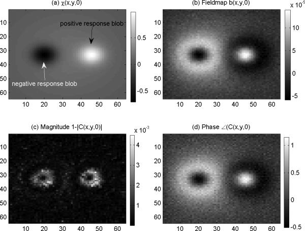
Numerical simulation of T2*MRI. a) A z-slice of the predefined 3D SM, (b) the fieldmap (the 3D convolution of (a) with an addition of Gaussian noise); (c) the MR magnitude (calculated from (b) by intravoxel dephasing) which bears a central dipping effect and an edge effect; and (d) the MR phase which conforms the fieldmap in (b).

Given the 3D phase volume (calculated by Eqs.(10) ), we calculated the fieldmap by Eq. (11). From the fieldmap, we performed the SM reconstruction by solving the 3D deconvolution in Eq. (12) by “filter truncation” and “TV iteration”. The results are shown in Fig. 4, from which we can see that: 1) the 3D phase volume looks morphologically different from the SM source that can be explained by a 3D convolution transformation in Eq.(7); 2) The TV solver produces a better restoration of SM source than does the truncation solver in the sense of less noisy and pattern replications. By using Eq. (20), we calculated the 3D spatial correlations between the reconstructed SM and the predefined SM, and obtained the quantitative results for this particular case: the TV solver produces a correlation of 0.993 and the truncation solver produces a correlation of 0.888. To present the SM reconstruction quantitatively for this particular case, we show a slice image as well as a scanline profile in Fig. 5.

Fig. 4.

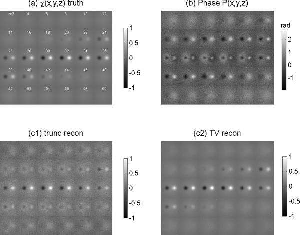
Demonstrations of CIMRI simulation (inverse mapping of Fig. 3). (a) the predefined 3D SM displayed with z-slices at z=2:2:60 (as used in Fig.(3a)), (b) the MR phase volume (as produced by T2*MRI in Fig. (3d)); (c1) the SM reconstruction by filter truncation solver (“trunc”); and (c2) the SM reconstruction by TV iteration solver (“TV”).

Fig. 5.

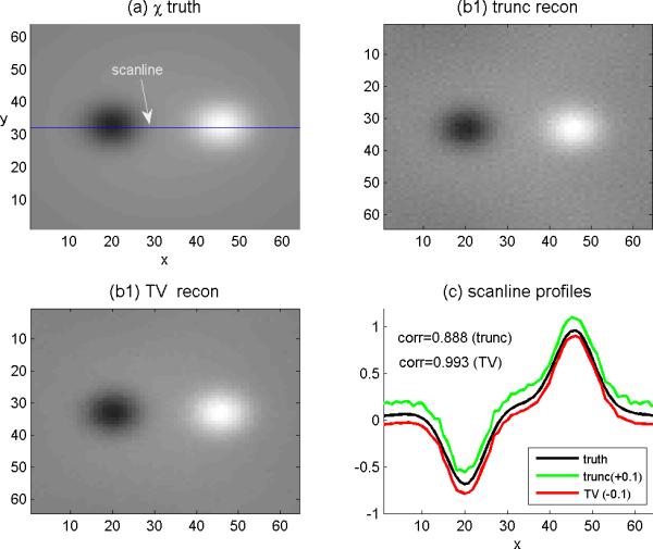
Scrutiny of CIMRI simulation with a slice image and a scanline profile. (a)A slice image of the predefined SM (where the horizontal line marks a scanline); (b1) the reconstructed slice image of SM by “trunc” solver, and (b2) by “TV” solver, and (d) the scanline profiles from (a), (b1) and (b2). The plots of “trunc” and “TV” reconstructions are shifted with offsets ±0.1to avoid overlapping display.

3.2 In vivo brain imaging experiment

In this subsection, we report on an in vivo brain imaging experiment and the real brain SM reconstruction by CIMRI. The brain imaging experiment was conducted with a healthy subject doing a finger-tapping visuomotor experiment in a Siemens Trio 3T scanner. An EPI complex sequence was used for scanning, with T_R/T_E=2000ms/29ms with isotropic voxels (2×2×2mm³). A brain FOV was localized to cover the motor cortex part (the parietal lobe and frontal lobe in brain) with a 3D matrix in size of 90×90×30. The brain functional imaging experiment produced a 4D complex dataset (90×90×30×165 after image crop) for a session of 330s scanning. We assume that we can reconstruct the brain SM source at each snapshot from a MR phase volume in the 4D dataset by our CIMRI model. In what follows, we demonstrate the CIMRI applications to brain SM reconstruction with an in vivo brain image captured at a snapshot.

Making sure that the phase image is phase unwrapped (the maximal phase angle is clearly less than π), we calculated the fieldmap by Eq.(11). From the fieldmap, we calculated the SM by the TV solver. In order to show the effect of regularization parameter λ value on the SM reconstruction, we repeated the TV program for a large range of λ values, from 30 to 5000. The overall results are presented with an axial slice of brain FOV in Fig.6, which consists of a raw MR magnitude (a), the raw phase counterpart (b1), and a smoothed phase (b2), and six SM reconstructions (c1-c6) with λ={30,50, 60, 100,500,5000}. By comparing the phase image (corresponding to the fieldmap) with the six SM reconstructions, we can see that the SM reconstruction may take on a smoothing effect at a very small λ and a contrast enhancement at a very large λ. In Figs 11 through 13 we provide the profiles for a scanline across the lateral ventricles (marked in Fig.6(a)) for quantitative scrutiny.

Fig. 6.

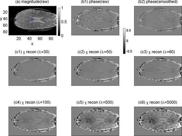
TV-regularized brain SM reconstruction from an in vivo experiment dataset. (a) an axial slice of the MR magnitude of brain imaging (where a vertical segment marks a scanline); (b1) the phase image slice; (b2) the smoothed phase; (c1-c6) the SM reconstruction from the phase (in (b1)) by using a large range of λ values. Note that the nonnegative magnitude image is displayed in a colorbar range of [0,1], and all the images are bipolar-valued and displayed in a colorbar range of [-0.6,0.6].

As discussed in Eq.(7), we understand that the convolutional magnetization plays an textual enhancement. Accordingly, the deconvolution is supposed to reveal a smoothing effect. We include a smoothed phase image in Fig.6(b2) (calculated from the raw phase image in Fig. 6(b1) by a local average) to show that the smoothing effect of 3D deconvolution looks different from the local average effect. The quantitative comparison between the deconvolution smoothing effect (λ=30) and the local average effect is shown in Fig. 7 with scanline profiles, where we can see that the smoothing effect of TV iteration cannot be achieved by a local averaging operation.

Fig.7.

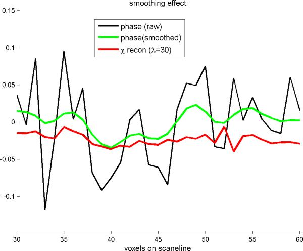
The scanline profiles extracted from Fig.6(b1)(b2)(c1) (The scanline is marked in Fig. 6(a)). It shows that the smoothing effect due to a small λ(=30) in TV iteration is different from that resulted from a local average.

In Fig.8 are shown the MR magnitude, the MR phase, and the SM reconstruction with λ=50. We can observe the following phenomena: 1) The phase suffers more noise than the magnitude; 2) the SM reconstruction is smoother than the phase; 3) the SM reconstruction takes on a distribution similar to the magnitude. In particular, the similarity between the magnitude and SM reconstruction allows us to consider the MR magnitude image as a good representation of the unknown SM source (albeit inexact).

Fig. 8.

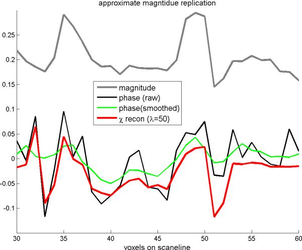
The scanline profiles extracted from Fig.6(a)(b1) (b2) and (c2). It shows that the reconstructed SM (with λ=50) assumes a morphological similarity to the MR magnitude(comparing the grayline and redline plots).

In Fig.9 are shown the contrast enhancement effect of large λ on SM reconstruction. As the parameter λ increases from 100, 500, to 5000, the scanline profiles increase in amplitude while roughly maintaining the distribution pattern, which manifests as textural enhancement in comparison with the MR phase image. In conclusion, the TV iteration reconstruction program may serve as a noise amplifier when a very large regularization parameter value is used.

Fig. 9.

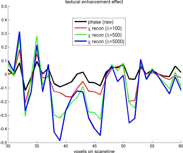
The scanline profiles extracted from Fig. 6(b1)(c4)(c5)(c6). It shows that the reconstructed SM with large λ values may reveal a textural enhancement effect on the phase image.

4. Discussion

The forward T2*MRI produces a complex-valued image where image contrast is attributed to the inhomogeneous susceptibility source. Due to the magnetization, spatial scanning, signal detection and image reconstruction, the overall process from the susceptibility source to MR image formation suffers noises. Since the complex modulo operation is a nonlinear operation, the MR magnitude image is a nonlinear transformation, with which we can explain the fact that the MR magnitude image is not an exact replica of the source. Consequently, we cannot reconstruct the susceptibility source from the MR magnitude image because the overall nonlinearity of MR magnitude image remains unclear and eludes an exact formulation so far. Fortunately, the MR magnitude map resembles the susceptibility map to a great extent albeit non-identical, which explains the rational of taking the MR magnitude image as a representation of the susceptibility source.

By decomposing the T2*MRI technology into two steps (see Fig. 1), it is possible to reconstruct the susceptibility source from a fieldmap by solving a 3D deconvolution problem. On one hand, the 3D deconvolution is an ill-posed problem because it involves a 3D kernel of point magnetic dipole field that is of bipolar-valued multilobular anisotropic distribution. On the other hand, the 3D deconvolution is a linear transformation, which allows to an inverse mapping in the sense of spatial conformance and error minimization. In small angle regime (exp(-iP)=1-iP, that is reachable by a small T_E), the phase angle remains unwrapped (|P|<π), such that the fieldmap takes on the MR phase map (different by a sale). As result, the susceptibility source reconstruction can be accomplished by deconvolving the 3D MR phase map with the point magnetic dipole kernel. In this paper, we simplify the fieldmap calculation under the small angle regime. In practice, the phase image may become wrapped (|P|>π) and the phase unwrapping is a necessary processing step prior to fieldmap calculation. In the phase-wrapped scenarios, it is also helpful to examine the nonlinearity associated with the fieldmap calculation from the phase map because any nonlinearity will jeopardize the susceptibility source reconstruction by CIMRI.

In comparison with the forward T2*MRI that is implemented by hardware scanning and software image reconstruction, the CIMRI model reverses the T2*MRI process by a pure computation. Since its goal is to reconstruct the unknown source with a high fidelity, the CIMRI serves as a tomographic susceptibility reconstruction from a MRI-scanned data, in a way similar to the CT that reconstructs the material density from x-ray projections. Following the rules of medical imaging system development, we conduct the numerical simulation to examine the CIMRI model in a quantitative manner. Prior to the clinical trial, it is necessary to validate the CIMRI with extensive numerical simulation (as rendered in section 3.1) and calibrate the CIMRI for a specific T2*MRI system with phantom experiments.

The crux of CIMRI lies in an ill-posed 3D deconvolution problem, for which we classify the solvers into three categories: 1) matrix inverse; 2) filter truncation, and 3) TV iteration. Although the matrix inverse solver is supported by the well-established matrix algebra and the filter truncation solver is supported by the filtering theory, both solvers struggle with the artifacts resulting from the effect of ill matrix regularization. Based on numerical simulation, we conclude that the split Bregman TV iteration algorithm outperforms the others in the following aspects: 1) It preserves edges; 2) It denoises the data such that there is no need to render image smoothing a priori (Note that the TV iteration method was originally developed for image denoising ¹⁶ and that smoothing is prone to suppress image features);3) It can accommodate large 3D phase maps per se without a convolutional matrix conversion; 4) It is an iteration algorithm that can produce a stable optimal restoration by avoiding the divide-by-zero problem, and in particular, the split Breman iteration guarantees fast convergence ^19-21.

While we appreciate the advantages offered by TV iteration, we also need to point out its disadvantages: 1) Its algorithm implementation is more complicated; 2) Although the Bregman iteration is of fast convergence (usually less than 20 iteration), its computation time is still longer than non-iteration solvers; 3) It may produce an over-smoothed solution if the regularization parameter value is too small (for example λ<20 in Fig.6(c1)); 4) it may bring back noise ^16-17 in a uniform region when the regularization parameter is too large (for example γ>1E3). We demonstrate the effect of regularization parameter λ with a brain susceptibility reconstruction from a MR phase map (see Figs. 6 through 9). For brain functional susceptibility reconstruction, we suggest a rule for λ selection: A proper λ value for the TV reconstruction program should produce a voxel susceptibility timecourse at an active region such that it highly correlates (or anticorrelates) with the external task stimuli paradigm. This is an ongoing research.

The 3D deconvolution associated with the CIMRI involves a point magnetic dipole kernel, which is in nature of 3D distribution. Therefore, CIMRI is optimal for volumetric susceptibility reconstruction from a MR phase volume. In practical implementation, the MR phase volume can be obtained by stacking 2D slices acquired by an EPI sequence. Usually, the slice-stacked volume is anisotropic (in-plane resolution is different from the across-plane resolution). An isotropic volumetric SM reconstruction can be achieved by acquiring an isotropic MR phase volume with isotropic voxels at a zero oblique angle and with no inter-slice gap. For dynamic brain BOLD fMRI study, the inter-slice time lag effect can be eliminated by an echo volume imaging (EVI) sequence ^33,34.

5. Conclusion

The underlying source of T2*MRI is the biomagnetic susceptibility map that is attributed to the static iron deposit in a structural state and the dynamic heme-iron perturbation associated with a functional state. The output of T2*MRI snapshot is a complex-valued volume, where the magnitude map is not an exact replica of the susceptibility source albeit similar, and the phase map is different from the source by a 3D convolution transformation (if the phase image remains unwrapped). In this work, we propose a CIMRI model for reconstructing the underlying susceptibility source of T2*MRI, which is implemented by two computational steps: “from MR phase map to fieldmap” and “from fieldmap to susceptibility map”. In the small angle regime where the phase angle remains unwrapped, the fieldmap conforms the phase map by a T_E-dependent scale. Upon the fieldmap calculation, the susceptibility map can be reconstructed therefrom by solving a 3D deconvolution problem (the inverse of convolutional magnetization), which however is an ill-posed inverse problem. We have addressed three kinds of 3D deconvolution solvers: matrix inverse, filter truncation, and TV iteration. Based on numerical simulation, we conclude that the 3D deconvolution problem associated with the CIMRI model can be well solved by a split Bregman TV-regularized iteration method.

Appendix A: Dimensionality curse of convolution-converted matrix

For a linear system, the input and the output is usually related by a convolution transformation. In the framework of linear transformation, an input-output relationship is represented by a matrix-vector multiplication format. In this appendix, we show that if we convert a convolution into a matrix-vector multiplication format, for 1D, 2D or 3D scenarios, we will encounter a very large converted 2D convolution matrix whose inverse is difficult to obtain. This situation is called dimensionality curse herein.

A.1 1D convolution b(x)= h(x)*χ(x)

Upon discreteness, we represent the 1D input χ(x), kernel h(x), and output b(x) by 1D vectors [χ]_1×L , [h]_1×N, and [b]_1×M, respectively. For a practical signal system, since its convolution kernel h(x) assumes a local spread distribution for a limited impulse response, therefore N<<L and N<<M. Accordingly, the 1D discrete convolution is expressed by

$$b\left[m\right]=\sum _{l}h[m-l]\chi \left[l\right],\text{for}\mid m-l\mid \le N$$ (A.1)

where the input vector and output vector is related by the 1D convolution kernel, not in matrix-vector format. By using a circular shift technique ⁹, we can construct a 2D matrix [h]_M×L from the 1D kernel [h]_1×N, that is,

$${\left[h\right]}_{M\times L}={\left[\begin{array}{ccccccc}\hfill h\left[1\right]\hfill & \hfill h\left[2\right]\hfill & \hfill \cdots \hfill & \hfill h\left[N\right]\hfill & \hfill 0\hfill & \hfill \cdots \hfill & \hfill 0\hfill \\ \hfill 0\hfill & \hfill h\left[1\right]\hfill & \hfill \cdots \hfill & \hfill h[N-1]\hfill & \hfill h\left[N\right]\hfill & \hfill \cdots \hfill & \hfill 0\hfill \\ \hfill 0\hfill & \hfill 0\hfill & \hfill \cdots \hfill & \hfill h[N-2]\hfill & \hfill h[N-1]\hfill & \hfill \cdots \hfill & \hfill 0\hfill \\ \hfill \cdots \hfill & \hfill \cdots \hfill & \hfill \cdots \hfill & \hfill \cdots \hfill & \hfill \cdots \hfill & \hfill \cdots \hfill & \hfill \cdots \hfill \end{array}\right]}_{M\times L}={\left[\begin{array}{c}\hfill circshift(h,0)\hfill \\ \hfill circshift(h,1)\hfill \\ \hfill \cdots \hfill \\ \hfill circshift(h,M)\hfill \end{array}\right]}_{M\times L}$$ (A.2)

where circshift(h,n) denotes a circular shift of the 1D vector h by n elements (right-ward shift). Thereby, we convert the 1D discrete convolution in (A.1) into the standard matrix-vector format as

$$\left[\begin{array}{c}\hfill f\left[1\right]\hfill \\ \hfill f\left[2\right]\hfill \\ \hfill \cdots \hfill \\ \hfill f\left[M\right]\hfill \end{array}\right]=\left[\begin{array}{cccc}\hfill h_{1,1}\hfill & \hfill h_{1,2}\hfill & \hfill \cdots \hfill & \hfill h_{1,L}\hfill \\ \hfill h_{2,1}\hfill & \hfill h_{2,2}\hfill & \hfill \cdots \hfill & \hfill h_{2,L}\hfill \\ \hfill \cdots \hfill & \hfill \cdots \hfill & \hfill \cdots \hfill & \hfill \cdots \hfill \\ \hfill h_{M,1}\hfill & \hfill h_{M,2}\hfill & \hfill \cdots \hfill & \hfill h_{M,L}\hfill \end{array}\right]\left[\begin{array}{c}\hfill u\left[1\right]\hfill \\ \hfill u\left[2\right]\hfill \\ \hfill \cdots \hfill \\ \hfill u\left[L\right]\hfill \end{array}\right]$$ (A.3)

Due to N<<L and N<<M, [h]_M×L takes on a large sparse matrix. The dimension relationship for (A.3) is governed by [M]=[M×L][L]. It is seen that the 1D convolution per se in (A.1) only involves N elements of [h]_1×N, whereas its implementation in matrix-vector format in (A.3) involves ML elements of [h]_M×L. Consequently, we encounter a dimensionality curse (ML>>N) if we reformat the 1D convolution into the matrix framework.

A.2 2D convolution b(x,y)= h(x,y)*u(x,y)

Let [χ]_Lx×Ly, [h]_Nx×Ny, and [b]_Mx×My denote the discrete versions for χ(x, y), h(x,y,), and b(x, y), respectively, then the 2D discrete convolution is represented by

$$b[m_x,m_y]=\sum _{l_x,l_y}h[m_x-l_x-l_y]\chi [l_x,l_y],\text{for}\mid m_x{l}_x\mid \le N_x,\mid m_y-l_y\mid \le N_y$$ (A.4)

It is seen that the input [χ] and the output [b] are represented in 2D matrix formats, but the input-output relationship is not represented in the standard matrix-vector format. In order to handle the 2D convolution with by using the matrix-based linear transformation framework, we need arrange the 2D image input and output into 1D vectors by a lexicographic ordering. Let [χ]_1×LxLy and [b]_1×MxMy represent the 1D vector versions of [χ]_Lx×Ly and [b]_Mx×My, respectively. We also need to construct a 2D matrix from the 2D convolution kernel by using the circular matrix technique ⁹. In the result, we reformat the 2D convolution in (A.4) into a matrix-vector format as

$$\left[\begin{array}{c}\hfill f_1\hfill \\ \hfill f_2\hfill \\ \hfill \cdots \hfill \\ \hfill f_{M_x{M}_y}\hfill \end{array}\right]=\left[\begin{array}{cccc}\hfill h_{1,1}\hfill & \hfill h_{1,2}\hfill & \hfill \cdots \hfill & \hfill h_{1,L_x{L}_y}\hfill \\ \hfill h_{21}\hfill & \hfill h_{22}\hfill & \hfill \cdots \hfill & \hfill h_{2,L_x{L}_y}\hfill \\ \hfill \cdots \hfill & \hfill \cdots \hfill & \hfill \cdots \hfill & \hfill \cdots \hfill \\ \hfill h_{M_x{M}_y,1}\hfill & \hfill h_{M_x{M}_y,2}\hfill & \hfill \cdots \hfill & \hfill h_{M_x{M}_y,L_x{L}_y}\hfill \end{array}\right]\left[\begin{array}{c}\hfill u_1\hfill \\ \hfill u_2\hfill \\ \hfill \cdots \hfill \\ \hfill u_{L_x{L}_y}\hfill \end{array}\right]$$ (A.5)

where the dimension relation is given by [M_xM_y]=[M_xM_y×L_xL_y][L_xL_y]. It is seen that the implementation of a 2D convolution in its original format in (A.4) involves N_xN_y elements of [h]_Nx×Ny, whereas in the converted matrix-vector format in (A.5), we need to deal with a matrix in size of [M_xL_y, L_xL_y]. Usually, N_x< L_x, N_x<M_x, N_y<L_y, and N_y<M_y hold for a 2D imaging system. The explosion in the dimension of the converted convolution matrix, that is, M_xL_yL_xL_y >> N_xN_y , is the so-called dimensionality curse for 2D convolution conversion.

A.3. 3D convolution b(x,y,z)= h(x,y,z)*χ(x,y,z)

In similar manner as done for the 2D convolution, we can convert a 3D discrete convolution

$$\begin{array}{c}\hfill b[m_x,m_y,m_z]=\sum _{l_x,l_y}h[m_x-l_x,m_y-1_y,m_z-l_z]\chi [l_x,l_y,l_z],\hfill \\ \hfill \text{for}\mid m_x-l_x\mid \le N_x,\mid m_y-l_y\mid \le N_y,\mid m_z-l_z\mid \le N_z\hfill \end{array}$$ (A.6)

into a matrix-vector format as given by

$$\left[\begin{array}{c}\hfill f_1\hfill \\ \hfill f_2\hfill \\ \hfill \cdots \hfill \\ \hfill f_{M_x{M}_y{M}_z}\hfill \end{array}\right]=\left[\begin{array}{cccc}\hfill h_{1,1}\hfill & \hfill h_{1,2}\hfill & \hfill \cdots \hfill & \hfill h_{1,L_x{L}_y{L}_z}\hfill \\ \hfill h_{21}\hfill & \hfill h_{22}\hfill & \hfill \cdots \hfill & \hfill h_{2,L_x{L}_y{L}_z}\hfill \\ \hfill \cdots \hfill & \hfill \cdots \hfill & \hfill \cdots \hfill & \hfill \cdots \hfill \\ \hfill h_{M_x{M}_y{M}_z,1}\hfill & \hfill h_{M_x{M}_y{M}_z,2}\hfill & \hfill \cdots \hfill & \hfill h_{M_x{M}_y{M}_z,L_x{L}_y{L}_z}\hfill \end{array}\right]\left[\begin{array}{c}\hfill u_1\hfill \\ \hfill u_2\hfill \\ \hfill \cdots \hfill \\ \hfill u_{L_x{L}_y{L}_z}\hfill \end{array}\right]$$ (A.7)

which is governed by a dimension relation [M_xM_yM_z]=[M_xM_yM_z×L_xL_yL_y][L_xL_yL_z]. The dimensionality course for a 3D convolution conversion lies in M_xM_yM_zL_xL_yL_y>>N_xN_yN_z.

A.4 Examples: dimensions of typical convolution matrices

Based on the matrix-vector representations for 1D, 2D, and 3D discrete convolutions, we notice that the converted convolution matrix suffers a dimensionality curse, which manifests as an rapid increase in dimension ([M_x, L_x], [M_xM_y, L_xL_y], and [M_xM_yM_z, L_xL_yL_z] corresponding to 1D [h]_1×N, 2D [h]_Nx×Ny, and 3D [h]_Nx×Ny×Nz, respectively). In table A, we provide specific numbers to show the dimensionality explosion problem, from which we understand that the dimensionality curse becomes the bottleneck of the 3D deconvolution problem by matrix inverse solver due to the difficult of calculating the inverse of a large matrix.

Table A.

Typical numerical examples for 1D, 2D, and 3D convolution system

	dim(χ)	dim(b)	dim(h)	remarks
1D	256	512	512x256	Typical 1D signal system
2D	256×256	256×256	65536×65536	Typical 2D image system
3D	64×64×32	64×64×32	131072×131072	Typical BOLD fMRI experiment

Appendix B: split Bregman TV regularization algorithm

It has been validated that the total variation (TV) regularization iteration is an excellent algorithm for image restoration in presence of noise and blurring. After first proposal in Rudin-Osher-Fatemi (ROF) model ³⁵, the TV regularization algorithm has been enriched in iteration convergence and speed by different strategies. Of particular improvement is the split Bregman iteration^16,19,20 (cf. http://www.math.ucla.edu/applied/cam/ for more details on theory and applications), we herein generalize the TV regularization to accommodate the 3D minimization problem in Eq. (18), which is copied therein for convenience.

$$\widehat{\chi }\left(\mathbf{r}\right)=\underset{\chi \in BV}{\min }{\Vert \chi \left(\mathbf{r}\right)\Vert }_{TV}+\frac{\lambda }{2}{\Vert B_{0}h\left(\mathbf{r}\right)\ast \chi \left(\mathbf{r}\right)-b\left(\mathbf{r}\right)\Vert }_2^2$$ (B.1)

It has been found that the non-differentiability problem can be effectively solved by an operator-splitting technique.

The split Bregman TV regularizartion is to decompose the TV minization problem in (B.1) into three subproblems with respect to three variables (d,v,χ), that is

$$\underset{\mathbf{d},\mathit{v},\chi }{\min }{\Vert \mathbf{d}\left(\mathbf{r}\right)\Vert }_{TV}+\frac{\lambda }{2}{\Vert v-b\Vert }_2^2\mathrm{s}.\mathrm{t}.\mathbf{d}\left(\mathbf{r}\right)=\nabla \chi \left(\mathbf{r}\right),v=h^{\ast }\chi$$ (B.2)

where the objective in (B.2) has been split into 2 terms: the first term is the TV norm of vector variable d (auxiliary) the second term is the fidelity expressed in L²-norm, which only depends on variable v (auxiliary); however, both d and v are still indirectly related variable χ via the constrainsts: d=∇χ and v=h*χ. By introducing two iteration parameters, a₁ and a₂, for these two constrainsts, we obtain the split Bregman iteration algorithm that is expressed as the following minimization problem ¹⁷

$$\underset{\mathbf{d},\mathit{v},\chi }{\min }{\Vert \mathbf{d}\left(\mathbf{r}\right)\Vert }_{TV}+\frac{\lambda }{2}{\Vert v-b\Vert }_2^2+\frac{{\gamma }_1}{2}{\Vert \mathbf{d}-\nabla \chi -{\mathbf{a}}_1\Vert }_2^2+\frac{{\gamma }_2}{2}{\Vert v-h^{\ast }\chi -a_2\Vert }_2^2$$ (B.3)

where γ₁and γ₂ are the Lagranger mulitiplies for the constraints. It is noted that the additonal terms of the iteratvie parameters, a₁ and a₂ are quadratic penalities which enforce the constrants. The solution of (B.5), which minimizes jointly over {‘d’, ‘v’, ‘ χ’} is approximated by alternatingly minimizing one variable at a time, that is, fixing v and χ while minimizing over d, then fixing d and χ while minimizing over v, and so on. Specifically, the three variable subproblems are solved as follows:

• 1)
  The d subproblem, with v and χ fixed, is

  $$\underset{\mathbf{d}}{\min }{\Vert \mathbf{d}\left(\mathbf{r}\right)\Vert }_{TV}+\frac{{\gamma }_1}{2}{\Vert \mathbf{d}-\nabla \chi -{\mathbf{a}}_1\Vert }_2^2$$ (B.4)

  Its solution is known in a closed form

  $$\mathbf{d}=\frac{\nabla \chi +{\mathbf{a}}_1}{\mid \nabla \chi +{\mathbf{a}}_1\mid }\max (\{\mid \nabla \chi +{\mathbf{a}}_1\mid -1∕{\gamma }_2,0\}$$ (B.5)

  This is the key subproblem that drives the minimization in (B.3).
• 2)
  The v subproblem, with d and χ fixed, is

  $$\underset{v}{\min }\frac{\lambda }{2}{\Vert v-b\Vert }_2^2+\frac{{\gamma }_2}{2}{\Vert v-h^{\ast }\chi -a_2\Vert }_2^2$$ (B.6)

  By performing derivative on (B.3) with respect to v, we obtain the optimal v condition

  $$\lambda (v-b)+{\gamma }_2(v-h^{\ast }\chi -a_2)=0$$ (B.7)

  which gives rise to the z solution in closed form

  $$v=\frac{h^{\ast }\chi +a_2+\frac{\lambda }{{\gamma }_2}b}{1+\frac{\lambda }{{\gamma }_2}}$$ (B.8)
• 3)
  The χ subproblem, with d and v fixed, is

  $$\underset{\chi }{\mathrm{nin}}\frac{{\gamma }_1}{2}{\Vert \mathbf{d}-\nabla \chi -{\mathbf{a}}_1\Vert }_2^2+\frac{{\gamma }_2}{2}{\Vert v-h^{\ast }\chi -a_2\Vert }_2^2$$ (B.9)

  The solution of χ can be obtained in Fourier doamin by

  $$\chi =IFT\left\{\frac{\frac{{\gamma }_2}{{\gamma }_1}{H}^{\ast }\cdot FT\{v-a_2\}-FT\{\nabla \cdot (\mathbf{d}-{\mathbf{a}}_1)\}}{\frac{{\gamma }_2}{{\gamma }_1}{H}^{\ast }\cdot H+{\left(2\pi k\right)}^2}\right\}$$ (B.10)

  where FT and IFT represents respectively Fourier transform and inverse Fourier transform, H=FT{h}, H* the complex conjuage of H, and k the coordinates in Fourier domain.

Conclusively, the split Bregman iteration regulaization solver for the minimization problem in (B.3) is implemented by the following algorithm:

Initialize χ=v=a2=0, d=a1=0, tol

Do

Solve the d subproblem by (B.5)

Solve the v subproblem by (B.8)

solve the χ subproblem by (B.10)

Update a1: =a1+∇χ-d

Update a2:=a2+h*χ-v

While ∥χcurrent-χprevious∥∞<tol

Output: χcurrent

References

- 1.Bushberg JT, Seibert JA, Leidholdt EM, Jr, Boone JM. The Essential Physics of Medical Imaging. second ed. Lippincott Williams & Wilkins; 2001. [Google Scholar]
- 2.Haacke EM, Brown R, Thompson M, Venkatesan R. Magnetic resonance imaging physical principles and sequence design. John Wiley & Sons, Inc; New York: 1999. [Google Scholar]
- 3.Haacke EM, Tang J, Neelavalli J, Cheng YC. Susceptibility mapping as a means to visualize veins and quantify oxygen saturation. Journal of magnetic resonance imaging : JMRI. 2010;32(3):663–676. doi: 10.1002/jmri.22276. [DOI] [PMC free article] [PubMed] [Google Scholar]
- 4.Shmueli K, de Zwart JA, van Gelderen P, Li TQ, Dodd SJ, Duyn JH. Magnetic susceptibility mapping of brain tissue in vivo using MRI phase data. Magnetic resonance in medicine : official journal of the Society of Magnetic Resonance in Medicine / Society of Magnetic Resonance in Medicine. 2009;62(6):1510–1522. doi: 10.1002/mrm.22135. [DOI] [PMC free article] [PubMed] [Google Scholar]
- 5.Li L, Leigh JS. Quantifying arbitrary magnetic susceptibility distributions with MR. Magn Reson Med. 2004;51(5):1077–1082. doi: 10.1002/mrm.20054. [DOI] [PubMed] [Google Scholar]
- 6.Li W, Wu B, Liu C. Quantitative susceptibility mapping of human brain reflects spatial variation in tissue composition. Neuroimage. 2011;55(4):1645–1656. doi: 10.1016/j.neuroimage.2010.11.088. [DOI] [PMC free article] [PubMed] [Google Scholar]
- 7.Wharton S, Schafer A, Bowtell R. Susceptibility mapping in the human brain using threshold-based k-space division. Magn Reson Med. 2010;63(5):1292–1304. doi: 10.1002/mrm.22334. [DOI] [PubMed] [Google Scholar]
- 8.Wu B, Li W, Guidon A, Liu C. Whole brain susceptibility mapping using compressed sensing. Magnetic resonance in medicine : official journal of the Society of Magnetic Resonance in Medicine / Society of Magnetic Resonance in Medicine. 2011 doi: 10.1002/mrm.23000. [DOI] [PMC free article] [PubMed] [Google Scholar]
- 9.Huettel SA, Song AW, McCarthy G. Functional magnectic resonance imaging. second ed. Sinauer Assoc.; 2009. [Google Scholar]
- 10.Fernandez-Seara MA, Techawiboonwong A, Detre JA, Wehrli FW. MR susceptometry for measuring global brain oxygen extraction. Magn Reson Med. 2006;55(5):967–973. doi: 10.1002/mrm.20892. [DOI] [PubMed] [Google Scholar]
- 11.Holt RW, Diaz PJ, Duerk JL, Bellon EM. MR susceptometry: an external-phantom method for measuring bulk susceptibility from field-echo phase reconstruction maps. J Magn Reson Imaging. 1994;4(6):809–818. doi: 10.1002/jmri.1880040612. [DOI] [PubMed] [Google Scholar]
- 12.Weisskoff RM, Kiihne S. MRI susceptometry: image-based measurement of absolute susceptibility of MR contrast agents and human blood. Magn Reson Med. 1992;24(2):375–383. doi: 10.1002/mrm.1910240219. [DOI] [PubMed] [Google Scholar]
- 13.de Rochefort L, Liu T, Kressler B, Liu J, Spincemaille P, Lebon V, Wu J, Wang Y. Quantitative susceptibility map reconstruction from MR phase data using bayesian regularization: validation and application to brain imaging. Magn Reson Med. 2010;63(1):194–206. doi: 10.1002/mrm.22187. [DOI] [PubMed] [Google Scholar]
- 14.Kressler B, de Rochefort L, Liu T, Spincemaille P, Jiang Q, Wang Y. Nonlinear regularization for per voxel estimation of magnetic susceptibility distributions from MRI field maps. IEEE Trans Med Imaging. 2010;29(2):273–281. doi: 10.1109/TMI.2009.2023787. [DOI] [PMC free article] [PubMed] [Google Scholar]
- 15.Schweser F, Deistung A, Lehr BW, Reichenbach JR. Quantitative imaging of intrinsic magnetic tissue properties using MRI signal phase: an approach to in vivo brain iron metabolism? Neuroimage. 2011;54(4):2789–2807. doi: 10.1016/j.neuroimage.2010.10.070. [DOI] [PubMed] [Google Scholar]
- 16.Chan T, Esedoglu S, Park F, Yip A. Recent developments in total variation image restoration. In: Nikos, Yunmei Chen, Paragios Faugeras, Olivier, editors. Handbook of mathematical models in computer vision. Springer; 2005. [Google Scholar]
- 17.Osher S, Burger M, Goldfarb D, Xu J, Yin W. An iterative regularization method for total variation-based image restoration. Multiscale Model. Simul. 2005;4(2):30. [Google Scholar]
- 18.Yeo DT, Fessler JA, Kim B. Motion robust magnetic susceptibility and field inhomogeneity estimation using regularized image restoration techniques for fMRI. Med Image Comput Comput Assist Interv. 2008;11(Pt 1):991–998. doi: 10.1007/978-3-540-85988-8_118. [DOI] [PubMed] [Google Scholar]
- 19.Goldstein T, Osher S. Report No. UCLA CAM Report. 2008;08-29 [Google Scholar]
- 20.Joshi SH, Marquina A, Osher SJ, Dinov I, Van Horn JD, Toga AW. Edge-Enhanced Image Reconstruction Using (TV) Total Variation and Bregman Refinement. Lect Notes Comput Sci. 2009;5567:389–400. 2009. [Google Scholar]
- 21.Liu B, King K, Steckner M, Xie J, Sheng J, Ying L. Regularized sensitivity encoding (SENSE) reconstruction using Bregman iterations. Magnetic resonance in medicine : official journal of the Society of Magnetic Resonance in Medicine / Society of Magnetic Resonance in Medicine. 2009;61(1):145–152. doi: 10.1002/mrm.21799. [DOI] [PubMed] [Google Scholar]
- 22.Spees WM, Yablonskiy DA, Oswood MC, Ackerman JJ. Water proton MR properties of human blood at 1.5 Tesla: magnetic susceptibility, T(1), T(2), T*(2), and non-Lorentzian signal behavior. Magn Reson Med. 2001;45(4):533–542. doi: 10.1002/mrm.1072. [DOI] [PubMed] [Google Scholar]
- 23.Milford FJ, Reitz JR, Christy RW. Foundations of electromagntic theory. Addison-Wesley; 1993. [Google Scholar]
- 24.Cheng YC, Neelavalli J, Haacke EM. Limitations of calculating field distributions and magnetic susceptibilities in MRI using a Fourier based method. Physics in medicine and biology. 2009;54(5):1169–1189. doi: 10.1088/0031-9155/54/5/005. [DOI] [PMC free article] [PubMed] [Google Scholar]
- 25.Gonzalez RC, Wood RE. Ditial image processing. Third ed. Prentice Hall; 2008. [Google Scholar]
- 26.Chen Z, Calhoun V. A computational multiresolution BOLD fMRI model. IEEE Trans. BioMed. Eng. 2011;58(10):5. doi: 10.1109/TBME.2011.2158823. [DOI] [PMC free article] [PubMed] [Google Scholar]
- 27.Chen Z, Calhoun VD. Two pitfalls of BOLD fMRI magnitude-based neuroimage analysis: non-negativity and edge effect. Journal of neuroscience methods. 2011;199(2):363–369. doi: 10.1016/j.jneumeth.2011.05.018. [DOI] [PMC free article] [PubMed] [Google Scholar]
- 28.Gonzalez RC, Wood RE. Ditial image processing. Addison-Wesley; 1992. [Google Scholar]
- 29.Li L. Magnetic susceptibility quantification for arbitrarily shaped objects in inhomogeneous fields. Magn Reson Med. 2001;46(5):907–916. doi: 10.1002/mrm.1276. [DOI] [PubMed] [Google Scholar]
- 30.Liu T, Spincemaille P, de Rochefort L, Kressler B, Wang Y. Calculation of susceptibility through multiple orientation sampling (COSMOS): a method for conditioning the inverse problem from measured magnetic field map to susceptibility source image in MRI. Magn Reson Med. 2009;61(1):196–204. doi: 10.1002/mrm.21828. [DOI] [PubMed] [Google Scholar]
- 31.Yao B, Li TQ, Gelderen P, Shmueli K, de Zwart JA, Duyn JH. Susceptibility contrast in high field MRI of human brain as a function of tissue iron content. Neuroimage. 2009;44(4):1259–1266. doi: 10.1016/j.neuroimage.2008.10.029. [DOI] [PMC free article] [PubMed] [Google Scholar]
- 32.Chambolle A, Lions PL. Image recovery via total variational minimization and related problems. Numer. Math. 1997;76:22. [Google Scholar]
- 33.Rabrait C, Ciuciu P, Ribes A, Poupon C, Le Roux P, Dehaine-Lambertz G, Le Bihan D, Lethimonnier F. High temporal resolution functional MRI using parallel echo volumar imaging. J Magn Reson Imaging. 2008;27(4):744–753. doi: 10.1002/jmri.21329. [DOI] [PubMed] [Google Scholar]
- 34.Yang Y, Mattay VS, Weinberger DR, Frank JA, Duyn JH. Localized echo-volume imaging methods for functional MRI. Journal of magnetic resonance imaging : JMRI. 1997;7(2):371–375. doi: 10.1002/jmri.1880070220. [DOI] [PubMed] [Google Scholar]
- 35.Rudin L, Osher S, Fatemi E. Nonlinear total variation based noise removal algorithms. Physics D. 1992;60:10. [Google Scholar]