

Abstract
Matrix factorization models are the current dominant approach for resolving meaningful data-driven features in neuroimaging data. Among them, independent component analysis (ICA) is arguably the most widely used for identifying functional networks, and its success has led to a number of versatile extensions to group and multimodal data. However there are indications that ICA may have reached a limit in flexibility and representational capacity, as the majority of such extensions are case-driven, custom-made solutions that are still contained within the class of mixture models. In this work, we seek out a principled and naturally extensible approach and consider a probabilistic model known as a restricted Boltzmann machine (RBM). An RBM separates linear factors from functional brain imaging data by fitting a probability distribution model to the data. Importantly, the solution can be used as a building block for more complex (deep) models, making it naturally suitable for hierarchical and multimodal extensions that are not easily captured when using linear factorizations alone. We investigate the capability of RBMs to identify intrinsic networks and compare its performance to that of well-known linear mixture models, in particular ICA. Using synthetic and real task fMRI data, we show that RBMs can be used to identify networks and their temporal activations with accuracy that is equal or greater than that of factorization models. The demonstrated effectiveness of RBMs supports its use as a building block for deeper models, a significant prospect for future neuroimaging research.
Keywords: RBM, ICA, DBN, intrinsic networks, fMRI
1. Introduction
The observation of temporally coherent blood oxygenation level-dependent (BOLD) signals from spatially distinct regions as obtained with functional magnetic resonance imaging (fMRI) gave rise to the notion of intrinsic networks (INs) (Biswal et al., 1995). Numerous INs describing functional connections at the macroscopic level have been identified consistently during both task and rest (Allen et al., 2011; Beckmann et al., 2005; Calhoun et al., 2008; Damoiseaux et al., 2006; Kiviniemi et al., 2009; Smith et al., 2009; Zuo et al., 2010). The study of INs has advanced our understanding of large-scale brain function in relation to task performance and diagnosis-related activity (Calhoun and Adali, 2012; Calhoun et al., 2012; Laird et al., 2003; Sorg et al., 2009).
A number of data-driven methods have been explored for identifying INs. Most common are single matrix factorization (SMF) models, including independent component analysis (ICA), principal component analysis (PCA), and non-negative matrix factorization (NMF), each of which model latent factors from fMRI data by solving a linear-mixing problem with various constraints on the factors. Outside the field of neuroimaging, recently developed deep models such as deep belief networks (DBNs) (Hinton and Osindero, 2006) and deep Boltzmann machines (DBMs) (Salakhutdinov and Hinton, 2009) have earned attention for surpassing state of the art performance in image and object recognition (Goodfellow et al., 2012; Krizhevsky et al., 2012; Lee et al., 2012), and speech and acoustic modeling (Mohamed et al., 2010). A restricted Boltzmann machine (RBM) (Hinton, 2000) is a probabilistic model that is frequently and effectively used to construct these deep models (Hinton and Osindero, 2006; Hinton and Salakhutdinov, 2006). RBM shares some practical similarities with SMF models, such as the relationship between data and INs through a single matrix. However, in distinction to SMFs, the RBM model is formulated as a density estimation problem rather than one of latent factor separation. Nevertheless, latent factors do arise in the solution to the RBM problem as a consequence of model structure.
DBNs have previously been used in biomedical data analysis for brain computer interface modeling (Freudenburg et al., 2011), generating visual stimuli with hierarchical structure (van Gerven et al., 2010), and for fMRI image classification (Schmah et al., 2008). In this paper, we introduce the RBM model and evaluate its potential as an analytic tool for feature estimation in functional imaging data. Motivated by the relative ease of constructing larger models out of the RBM blocks, in this initial work we investigate whether RBM by itself is capable of competing with SMF models, in particular ICA. We first evaluate RBM performance relative to that of several well-known SMF models using synthetic fMRI data. Subsequently, we perform a detailed comparison between RBM and ICA on real task fMRI data. Our findings suggest that the RBM model alone is at least as powerful as ICA, supporting further applications in neuroimaging, particularly as a building block for deeper models.
2. Methods
In the following sections we detail the basic framework of RBMs — the learning objective, graphical representation, and parameter meaning in the context of fMRI —and compare it to popular factorization models including Infomax ICA (Bell and Sejnowski, 1995), PCA (Hastie et al., 2001), sparse PCA (sPCA) (Zou et al., 2006), and sparse NMF (sNMF) (Potluru et al., 2013). We note that other novel methods, such as dictionary learning (Varoquaux et al., 2011), also do well against these SMF models, but are not considered here for brevity. A more in depth treatment of the motivations, theory, and methods behind RBMs for parameter estimation are covered in Appendix A and Appendix B, along with motivation for other model and learning parameters Appendix C.
2.1. Single Matrix Factorization
Most of the popular methods for inferring INs from fMRI data have as their core assumption the existence of hidden factors that are linearly mixed to produce the observed data. In practice, this often amounts to considering data as an M × N matrix X of N M-dimensional observations and finding its best factorization as a mixing matrix and a matrix of hidden factors under a set of constraints.
The factorization problem can be formulated as
| (1) |
where S is a C × N matrix of C hidden factors and D is a C × M demixing matrix. Constraints specific to each SMF model considered in this work are summarized in Table 1.
Table 1.
The common problem solved by all considered SMF models and their unique constraints, where si. is the ith row of S; ⫫ denotes statistical independence; denotes a C × C identity matrix; and λ is the sparsity parameter.
| Find S and D such that S ≈ DX | ||
|---|---|---|
| Solve | Constraints | Description |
| ICA | Si. ⫫ sj., ∀i ≠ j | optimize independence |
| PCA | maximize variance | |
| enforce orthogonality | ||
| sPCA | maximize variance | |
| enforce orthogonality | ||
| ∥D∥1 ≤ λ | enforce sparsity | |
| sNMF | Sij ≥ 0, Dij ≥ 0 | enforce nonnegativity |
| ∥D∥1 ≤ λ | enforce sparsity | |
2.2. Restricted Boltzmann Machine
In contradistinction to the SMF models summarized in Table 1, RBM cannot be formulated as a problem of fitting a matrix of factors to the data. RBM is a probabilistic energy-based model, and the objective is to fit a probability distribution model over a set of visible random variables v to the observed data. General energy-based models define the probability by the energy of the system, E(v), such that,
| (2) |
where Z is a normalization term (Bengio et al., 2012).
RBM models the density of visible variables v by introducing a set of conditionally independent hidden variables h, such that the probability distribution becomes:
| (3) |
By introducing conditionally independent random hidden variables h and enforcing conditional independence on the observable variables v, RBM models the data through latent factors expressed only through interactions between visible and hidden variables. This improves interpretability and expressive power, and importantly makes estimation of the probability density computationally feasible (Hinton, 2000). Note, though, that the variables h are entirely hidden and not expressed in the final probability distribution of the data, as can be seen in Equation 3, where they have been marginalized out.
For modeling data that is real valued and approximately normally distributed, it is appropriate to define the energy function as:
| (4) |
The three terms in this function describe the energy associated with: 1) the interaction strengths, Wij, between each visible variable vi and hidden variable hj, 2) the visible units vi and their biases, ai (Gaussian center. See Equation B.2 in Appendix B), and 3) the hidden units hj and their biases, bj (Linear o set. See Equation A.5 in Appendix A). The parameter σi is the standard deviation of a quadratic function for each vi centered on its bias ai, effectively modeling the Gaussian distribution of each voxel. Note that there are no visible-visible nor hidden-hidden interaction terms in the energy, highlighting the conditional independence between each set of units.
2.3. Graphical Representations
Both SMF models and RBM can be represented by different types of supporting graphs, as shown in Figure 1. For SMF models, the graph is purely schematic: nodes represent the processing steps of the mixing in Equation 1, and the edges represent the multiplicative factors D. RBM, in contrast, can be defined as a graphical model, represented by a bipartite graph. Nodes represent the visible and hidden random variables and the edges represent the interaction terms between hidden and visible variables, W. Despite the different meaning of these graphs, one can note their similar structure, especially the relationship of D and W (in transpose) to latent factors, a theme we will revisit in subsequent sections.
Figure 1.

Graphical representation of SMF and RBM. The graph of SMF models represents the demixing of the data with the demixing matrix (D) as in Equation 1, while the graph in RBM represents the interaction terms (W) between visible (v) and hidden (h) variables. xi· are the rows of X and sj·. are the rows of S.
2.4. fMRI Context
In the context of fMRI, various components of the SMF graph represent the spatial maps (SMs) and time courses (TCs) of INs. For spatial-demixing models where temporal factors are mixed to produce spatial representations (PCA and NMF as implemented here), the mixing matrix quantities are related in the following way: X is a voxels-by-time data matrix, D is the source-by-voxels spatial demixing matrix, and S is the source-by-time matrix of temporal sources. The jth row of S, sj·, represents the jth TC, and the SMs are represented by the columns of the mixing matrix, D−1.
For Spatial ICA (as ICA is commonly applied to fMRI data), time and space are in transpose and the SMF represents temporal demixing of spatial factors: X is a time-by-voxels data matrix, D is the source-by-time temporal demixing matrix, and S is the source-by-voxel matrix of spatial sources. The jth row of S, sj·, represents the jth SM, and the TCs are represented by the columns of the mixing matrix, D−1.
In RBM, the visible variables v span the same space as a single volume of fMRI data x·n; that is, each variable, vi, corresponds to a single voxel. The number of hidden variables, h, corresponds to the number of INs (latent factors). Each hidden factor generates (when RBM is sampled from) or recognizes (when the data is presented) a coherent pattern of voxels. Thus, the weights from a single hidden unit j to all voxels , w·j, represents a spatial receptive field, or in the context of INs, its SM.
As a model of probability distribution over v, RBM does not incorporate time courses explicitly. We can, however, use a trained RBM and re-interpret the graphical structure as a feedfor-ward rather than undirected model. That is, we re-interpret the RBM graph as an SMF model (Figure 1) and treat WT as a demixing matrix. We then compute time courses as a linear function of WT (see Figure 3):
| (5) |
where the columns of S are the TCs for each SM. Notably, RBM is regularly and effectively used as a pretraining method for feedforward deep models (Hinton and Osindero, 2006; Hinton and Salakhutdinov, 2006) in this exact manner.
Figure 3.
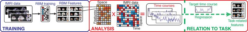
Pipeline for RBM training and analysis. An RBM is first used to obtain intrinsic networks (INs), each with a corresponding SM estimate. The model parameters are then used to forward propagate data onto the INs; this is done by matrix-multiplying the data (space × time) with the SM estimates (features × space), producing time course estimates specific to each IN. For task-related data (as with real fMRI data in Section 2.7), multiple regression with time courses derived from the experimental protocol is used to identify task-related INs.
For a more in depth treatment of the loss functions for RBM and SMF models covered in this work, please refer to Table A.3 in the Appendices.
Figure 2 highlights the steps of the RBM learning algorithm, the details of which are provided in Appendix A. The learning gradient is computed from a single datapoint, while the algorithm cycles through the complete dataset (all subjects together); a single cycle is called an “epoch”. For each data point presentation, each visible variable is assigned the value of the corresponding voxel. Then, a truncated, iterative version of Gibbs sampling called contrastive divergence (CD, see Appendix A.2) is applied to the complete set of variables. This is done in an alternating sequence of hidden and visible variables, using current values of the weights to calculate sampling probabilities of each layer.
Figure 2.

Steps of the RBM algorithm: 1) Set the visible units equal to a data vector. 2) Use contrastive divergence (CD) to first infer hidden states given data, then generate hypothetical data, which is used to update the hidden states. 3) Use the visible and hidden states during CD to calculate the parameter gradients. 4) Modify parameters using the gradient values. 5) Repeat steps 1 through 4 until parameters converge.
The difference between the values of the hidden and visible variables at the beginning and the end of the Gibbs chain is used to calculate the learning gradients, which are used to update the values of the weights before the next fMRI data point is presented. In addition, other penalty functions, such as L1 penalty on the weights (see Appendix C.1) or sparsity of simultaneously active hidden units can be applied here. The gradient update is scaled by a learning rate hyper-parameter which can greatly influence learning convergence.
Typically, convergence of model parameters requires many epochs of learning. To improve speed and take advantage of parallel and GPU processing, the learning algorithm can be improved by processing data in batches (often referred to as minibatches in the literature), where several data points are processed in parallel with their contributions to the learning gradient averaged. For batches of n data points, n RBMs are trained in parallel and the mean gradient over the batch is used in parameter estimation (Hinton, 2010).
Data samples from the probability distribution defined by the energy can be generated via alternating Gibbs sampling. This is typically done by initializing random variables at a random or specified state (in the case of generating data specific to an IN of interest) and running a Gibbs chain until convergence, using the set of visible variables as the generated sample.
2.6. Synthetic Data Analysis
We first considered synthetic data in order to objectively evaluate RBM performance. We trained RBMs using the publically available deepnet implementation (https://github.com/nitishsrivastava/deepnet) and compared estimation performance with a widely-used implementation of spatial ICA in GIFT (http://mialab.mrn.org/software/gift/), along with implementations of PCA and sPCA (Sjöstrand, 2005) and sNMF (Potluru et al., 2013). The SimTB toolbox (Erhardt et al., 2012) was used to generate synthetic 3D (x, y, and t) fMRI-like data from linear combinations of 27 distinct spatial sources with 2D Gaussian spatial profiles. Rician noise was added to the combined data to achieve a contrast-to-noise ratio between 0.65 and 1. Data for 20 artificial “subjects” consisting of 128 volumes were generated from the auditory oddball (AOD) example experiment from the toolbox, in which a subset of sources are modulated by “standard”, “target”, and “novel” events with different weights. Additionally, two sources are modulated by nearly identical noise (spike) events. Thus, source activations are temporally correlated to some degree, though each has its own unique behavior.
Twelve sets of SimTB data were produced by varying a SimTB source “spread” parameter, which changes the relative spatial standard deviation of each source. Increase in spread increases the percentage overlap between features; we define the total overlap of a set of sources as the percentage of voxels in which more than one source contributes over 0.5 standard deviations. We constructed datasets with overlap ranging from 0.3 (minimal spatial overlap between sources) and 0.88 (very high overlap).
RBMs were constructed with 16936 Gaussian visible units (one for each voxel), and a variable number of hyperbolic tangent hidden units (see below). Hidden unit nonlinearity choice is discussed in Appendix C.2, and learning hyperparameters are discussed in more detail in 4.3. The L1 decay rate was set to 0.1 based on performance over multiple experiments, and the learning rates for different model orders were determined as per Section 4.2. The RBMs were then trained with a batch size of 5 for approximately 75 epochs to allow for full convergence of the parameters.
For a set of synthetic data with moderate overlap (0.52), we constructed RBMs with the number of hidden units ranging from 10 to 80 in steps of 10 in order to study the dependence of performance on model order. To investigate the dependence of performance on spatial overlap, we used a single model order of 64, because this value exceeds the true data dimensionality (beneficial due to the presence of additive noise), and the GPU implementation of RBM favors model orders of powers of 2. Identical model orders were used for the SMF models for equivalent comparisons. For group ICA, the data was preprocessed using a two-step PCA by reducing each subject data to 120 principal components, then reducing the concatenated subject principal components again to the final component number. For sPCA, we chose the sparsity by counting the number of voxels in each ground truth source that were above one standard deviation, then taking a rough average of those counts: 1000. For sNMF, a sparsity of 0.7 was used based on performance over multiple experiments.
The RBM analysis pipeline (in the context of fMRI) is illustrated in Figure 3. After acquiring SM estimates from RBM learning, we construct a spatially-demixing SMF model from the learned RBM parameters and forward-propagate the whole dataset for each subject to obtain subject-specific time course (TC) estimates as per Equation 5. For ICA, TCs were produced using dual-regression, while for other SMF models, TCs were produced using their appropriate projections. Finally, due to the relevance in current fMRI research (e.g., Allen et al. (2011)), functional network connectivity (FNC) was computed as cross-correlations using subject-specific TCs.
Each of the models were run over 10 different random seeds. The SM, TC, and FNC estimates from each model were compared to those of the ground truth SimTB sources and features were matched to ground truth sources by solving the assignment problem using the Hungarian algorithm (Burkard et al., 2009), optimizing matches based on the absolute value of SM correlation to the ground truth. Estimation performance was determined based on the SM and TC correlations to the ground truth.
2.7. AOD FMRI Analysis
Based on results from simulations (see Section 3), real fMRI analysis was only performed with RBM and ICA.
Data used in this work comprised task-related scans from 28 healthy participants (five females), all of whom gave written, informed, IRB-approved consent at Hartford Hospital and were compensated for participation.
All participants were scanned during an auditory oddball task (AOD) involving the detection of an infrequent target sound within a series of standard and novel sounds. More detailed information regarding participant demographics and task details are provided by Calhoun et al. (2008) and Swanson et al. (2011).
Scans were acquired at the Olin Neuropsychiatry Research Center at the Institute of Living/Hartford Hospital on a Siemens Allegra 3T dedicated head scanner equipped with 40 mT/m gradients and a standard quadrature head coil. The functional scans were acquired transaxially using gradient-echo echo-planar-imaging with the following parameters: repeat time (TR) 1.50 s, echo time (TE) 27 ms, field of view 24 cm, acquisition matrix 64 × 64 , flip angle 70°, voxel size 3.75 × 3.75 × 4 mm3, slice thickness 4 mm, gap 1 mm, 29 slices, ascending acquisition. Six “dummy” scans were acquired at the beginning to allow for longitudinal equilibrium, after which the paradigm was automatically triggered to start by the scanner. The final AOD dataset consisted of 249 volumes for each subject.
Data underwent standard pre-processing steps using the SPM 5 software package (see Calhoun et al. (2008) for further details). To remove voxels outside the brain, masks were determined for each subject using AFNI’s 3dAutomask. A group mask was then determined as those voxels that were present in 70% of the subject masks, retaining 70969 voxels. Finally for each subject dataset, the voxels were variance normalized before concatenating into the dataset used for RBM training. The final fMRI dataset was composed of a total of 6972 volumes (28 subjects with 249 each).
The RBM was constructed using 70969 Gaussian visible units (matching the number of voxels in the data) and we again used 64 hyperbolic tangent hidden units (See Section 4.2 for details on model order and Appendix B for details on hidden unit choice). The hyper parameters ε for learning rate and λ for L1 weight decay were selected to optimize reduction of reconstruction error over training and spatial map size respectively. The RBM was then trained with a batch size of 5 for approximately 100 epochs to allow for full convergence of the parameters.
We labeled INs based on the Talairach-Tournoux (TT) atlas as provided in AFNI, and excluded features which had a high overlap with white matter, ventricles, or brain edges. In order to compute TCs for each fMRI feature, we subtracted the mean from each fMRI volume time series and filtered it through the trained RBM (via matrix multiplication, as in the simulation). This was done to better compare to ICA, where the mean is removed at the PCA pre-processing stage.
For ICA, spatio-temporal (dual) regression was used to produce TCs (Erhardt et al., 2011). ICA SMs were similarly manually filtered for white matter, ventricles, and other artifacts. To facilitate comparisons between the models, RBM and ICA SMs were cross correlated spatially; features with a spatial correlation exceeding 0.4 were considered matches.
For both RBM and ICA, subject-specific TCs were cross correlated to yield FNC matrices. TCs were also used to identify task-related features. First-level regression models fitting IN time courses to target and novel experimental designs were followed by second-level t-tests on the beta values (Figure 3).
3. Results
We first summarize our comparisons of RBMs with SMF models for synthetic data, then present a more in-depth comparison of RBMs and ICA for synthetic and real fMRI data.
3.1. Synthetic Results
Figure 4A shows the SM and TC estimation accuracy for RBM, ICA, sNMF, sPCA, and PCA. Considering both SM and TC estimation, all models other than PCA perform rather well, though show different sensitivities to model order. For RBM, both SM and TC estimation accuracy increase with model order. For ICA, SM and TC accuracy appears to peak around a model order of 40, and decreases slightly at higher model orders. SNMF, in contrast, shows increased SM but decreased TC accuracy with increasing model order. SPCA is relatively insensitive to increases in model order beyond the true dimensionality. Figure 4B demonstrates that types of estimation errors observed, which tend to be linear combinations of ground truth SMs and erroneous negative background. PCA tended to find non-sparse features, some similar to those found by sPCA, but of low quality overall. For lower model orders, we observed that RBM, sNMF, and sPCA tended to estimate SMs which appeared to be linear combinations of ground truth spatial maps. ICA, in contrast, would find a subset of relatively accurate SMs, albeit with larger spatial volume.
Figure 4.

A) Correlation of SM (left) and TC (right) estimates to the ground truth for all models as a function of model order. Lines indicate average correlation across all datasets (and “subjects” for TCs) with a spatial overlap at 0.52, and the color-fill indicates two standard errors around the mean. B) Contours of all ± SMs (top row) given a thresholded of 0.4 and examples of individual SMs for all models (bottom rows) at a model order of 64 and dataset overlap of 0.52. Typical SM quality between models was very similar and notable examples are shown. C) SM and TC accuracy as a function spatial overlap, at a model order of 64.
When taking overlap into consideration (Figure 4C), all models other than PCA showed comparable results, with ICA slightly performing better for SMs and RBM performing slightly better on TCs than ICA. Other than PCA, all models showed improved performance with overlap, possible due to a reduction in the relative influence of noise as sources increased in spatial extent. Time course estimations showed very little dependence on source overlap.
As ICA exhibits equal or better performance than the other SMF models and is arguably the most popular SMF models used to estimate INs, we continue with a more detailed analysis of RBM in comparison to ICA. Figure 5 provides examples of specific SM estimates for RBM and ICA in a sample dataset. Positioned above in the figure are example RBM/ICA SM pairs that matched to the same ground truth. RBM SM estimates suffer not due to shape, but due to capturing shared temporal information in SMs when ground truth source pairs have strong temporal correlations (e.g., feature i, upper right corner of example features). Thus, even when RBM features are outperformed by equivalent ICA features in SMs, RBM time courses may be more accurate.
Figure 5.

Examples of estimated SMs for RBM and ICA. Each SM is independently variance-normalized; red and blue denote positive and negative values, respectively. Above: example features show SM quality; text indicates spatial and temporal correlations to the ground truth. Middle: Scatter plot between FNC ground truth (GT) and estimation biases in cross-correlations between SMs (estimated-truth). Example pairs for RBM with biases in each direction are shown. RBM feature i is involved in a large proportion of strongly biased spatial cross correlations. Bottom: example features showing scenarios where RBM combines sources with high temporal correlation into a single features (left), and where ICA fails to estimate some ground truth features (right).
To make this point more evident, an analysis of RBM spatial bias is provided in the middle of Figure 5. A scatter plot comparing ground truth FNC versus estimated spatial cross correlations shows that RBM biases spatial cross correlation in the direction of FNC. For example, a pair of RBM features (ii and iii) in Figure 5 show (erroneous) spatial overlap with each other due to their relatively high temporal cross-correlation. An anti-correlating pair (iv) in contrast shows (erroneous) negative spatial overlap. An extreme case of RBM spatial bias can be seen at the bottom of Figure 5 and occurs when a set of sources have very high FNC values, ~ 0.99). In this case, RBM has completely merged the two features. Notably, ICA correctly estimates the SMs as separate features, but does not estimate the TCs well.
Though ICA SMs typically capture shape quite well, they often include more erroneous background features, seen as negative voxels in blue in Figure 5. Additionally, ICA failed to estimate a SM as a unique component, and instead merged it into the negative background of another SM (labeled v). While the resulting SM is similar to a pair in RBM (iv), the two features involved are not temporally correlated (~ 0.02). Rather, we believe the merging is due to the low kurtosis of the source, flat spatial distribution, and spatial overlap between the two sources.
Figure 6 shows FNC estimation bias as a function of the ground truth FNC for RBM and ICA. Both ICA and RBM mis-estimate the FNC between a number of features. In this particular simulation, RBM overestimates FNC with stronger ground truth FNC, while ICA underestimates the FNC for the same pairs of components (see C in Figure 6). The RBM FNC results correspond well with our understanding of the RBM features and construction of TCs: because RBM overestimates spatial cross-correlation between pairs with high FNC, this in turn will induce extra temporal cross-correlation when we calculate TCs via forward-propagation (matrix multiplication between data and SMs). For ICA, the FNC and spatial correlation biases are dependent on the exact configu-ration of the spatial maps (see Figure 7F of Allen et al. (2012b)) due to the constraint of spatial independence, thus biases are more difficult to predict in real datasets where the ground truth is not known.
Figure 6.

A 2D histogram showing the relationship between ground truth (GT) FNC and FNC estimation bias (estimated -true) for RBM and ICA estimates on the same synthetic dataset overlap shown in Figure 5. Note that density is log-scaled to improve visualization. Features A) and B) indicate instances where both RBM and ICA overestimate (positively bias) FNC values that are close to zero. Feature C) denotes cases where RBM overestimate positive FNC values (more so than ICA) and feature D) shows both methods underestimating some negative correlations.
Figure 7.

Groups of spatial maps of intrinsic networks estimated by RBM from fMRI data. INs were divided into groups based on their anatomical and functional properties. For visualization, each SM was thresholded at greater or less than 2 standard deviations. Estimated intrinsic networks are 1) thalamus; 2) inferior frontal gyrus (IFG); 3) middle temporal gyrus (MTG); 4) inferior temporal gryus (ITG); 5) middle cingulate cortex (MCC, overlapping with insula+MCC IN); 6) insula; 7) superior temporal gyrus (STG); 8) supramaginal gyrus (SMG); 9) superior parietal lobule (SPL); 10) precentral gyrus (PreCG); 11) postcentral gyrus (PoCG); 12) paracentral lobule (ParaCL); 13) supplementary motor area (SMA); 14) inferior parietal lobule (IPL); 15) middle frontal gyrus (MiFG); 16) medial frontal gyrus (MFG); 17) inferior frontal gyrus (IFG); 18) superior frontal gyrus (SFG); 19) lingual gyrus (LingualG); 20) inferior occipital gyrus (IOG); 21) cuneus; 22) calcarine gyrus (CalcarineG); 23) middle occipital gyrus (MOG); 24) precuneus; 25) anterior cingulate cortex (ACC); 26) posterior cingulate cortex (PCC); 27) angular gyrus (AG); 28) cerebellum (CB). The FNC (temporal correlation matrix) averaged across subjects is shown on the left. The numbers on the diagonal of the FNC matrix are RBM component number.
3.2. Real fMRI AOD Results
From the RBM features, we removed components corresponding to artifacts (edges, ventricles, or white matter regions), and identified 46 INs with peaks in grey matter. Based on their temporal correlations, known anatomical and functional properties, and cross-referencing to prior work (Allen et al., 2012a), we manually arranged INs into 8 separate groups. The grouped INs as well as the FNC are shown in Figure 7. We labelled groups based on their spatial properties as: 1, subcortical; 2, temporal + frontal cortices; 3, temporal cortex; 4, somatomotor cortex; 5, frontoparietal cortex; 6, visual cortex; 7, default mode network (DMN); and 8, cerebellar networks.
3.2.1. Spatial Analysis
Following removal of artifact components from the ICA results, we identified 38 INs with peaks in grey matter.
A comparative overview between RBM vs ICA components is provided in Table 2. Overall, RBM found a larger proportion of identifiable grey-matter features, while ICA distinguished more distinct white matter regions. Using spatial cross-correlation, we identified 52 RBM/ICA feature pairs (including artifacts, many-to-one) which had spatial cross correlations above 0.4. Ten such pairs are presented in Figure 8. Many of the RBM features showed supra-threshold spatial correlation to more than one ICA feature (and vice versa), indicating that the two models identified unique sets of latent factors (see Table C.5 for additional details). For instance, RBM and ICA show slight differences in combinations of DMN regions (AG, PCC, MiFG, MFG, and ACC) (Figures 15(a) and 15(b)), though overall the DMN sub-networks are very similar. Analysis and visual inspection of feature pairs generally shows RBM features are more sparse than those of ICA. In addition, RBM features are predominantly of a single sign, as opposed to ICA features which contain regions of both signs exceeding 2 standard deviations, similar to our observations in synthetic data.
Table 2.
Counts of grey matter (GM) features, white matter (WM) features, ventricles, and other artifacts in RBM and ICA results. Component classification was performed manually.
| GM | WM | Ventricles | Other | |
|---|---|---|---|---|
| RBM | 46 | 5 | 5 | 8 |
| ICA | 38 | 15 | 6 | 5 |
Figure 8.

Sample pairs of RBM (top) and ICA (bottom) SMs thresholded at 2 standard deviations. Pairing was done with the aid of spatial correlations, temporal properties, and visual inspection. Values indicate the spatial correlation between RBM and ICA SMs.
Figure C.15.

Default mode networks identified by RBM (a) and ICA (b) and p-values to target stimulus. t and p values are from multiple regression to target time courses.
3.2.2. Temporal Analysis
RBM features identified as part of the temporal and motor cortices, as well as those commonly associated with cognitive control (insula and middle cerebral cortex) showed the largest covariation to target stimuli, while only temporal cortex and supramarginal gyri showed positive statistically significant correlation to novel stimuli (see Table C.5 for details). RBM features negatively modulated by task are those which belong to the default mode network (DMN) and visual cortices. In general, these findings are consistent with the ICA results presented here and reported previously (Calhoun et al., 2008). A direct quantitative comparison of task-relatedness between RBM and ICA TCs again suggests the methods are comparable, as seen in Figure 9 where we plot the target and novel t-statistics for RBM and ICA feature pairs with spatial correlation above 0.4 in Figure 9. Wilcoxon signed rank test on the absolute value of the t-statistics suggests no significant difference in magnitude (p-values of 0.27 and 0.24 for targets and novels, respectively).
Figure 9.

Target (left) and novel (right) t-statistics for RBM and ICA feature pairs with spatial correlations above 0.4. The red line indicates unity.
The FNC matrices for both RBM and ICA are provided in Figure 10, where the ordering of components is performed separately for each method. For RBM, modularity is more apparent, both visually and quantitatively. FNC Modularity, as defined in Rubinov and Sporns (2011), averages 0.40 ± 0.060 across subjects for RBM, and 0.35 ± 0.056 for ICA. These values are significantly greater for RBM (t = 7.15, p < 1e−6, paired t-test). Also note that the scale of FNC values for RBM and ICA is different, echoing the simulation results wherein RBM overestimated the magnitude of strong FNC values.
Figure 10.

FNC determined from RBM (left) and ICA (right), averaged over subjects. Note that the color scales for RBM and ICA are different (RBM shows a larger range in correlations). The FNC matrix for ICA on the same scale as RBM is also provided as an inset (upper right). Feature groupings for RBM and ICA were manually determined separately, using the FNC matrices and known anatomical and functional properties. Numbers on the diagonal refer to the feature number in the model.
4. Discussion
4.1. Overview
In this paper, we investigated RBM as a model for separating spatially coherent sources from fMRI data, a problem which is currently addressed with SMF models. Our simulations show that RBM performs competitively against all SMF methods tested. Detailed comparisons with synthetic data show relatively comparable performance between RBM and ICA, with RBM providing slightly improved TC estimation and slightly worse SM accuracy over some ranges of model orders. We observe that the loss in spatial accuracy comes not from an inability to identify features, but from a tendency of RBMs to capture strong temporal correlations within the spatial domain. Thus, in the worst case, RBM SM estimates were still highly interpretable as combinations of temporally correlated ground truth sources.
Applied to real fMRI data collected during an AOD task, RBM and ICA again yielded similar sets of INs, consistent with networks found in a variety of task and resting-state experiments (Allen et al., 2011; Beckmann et al., 2005; Calhoun et al., 2008; Damoiseaux et al., 2006; Kiviniemi et al., 2009; Smith et al., 2009; Zuo et al., 2010). Though RBM and ICA showed some variations in features (see Figures 8, 15(a), and 15(b)), the TCs of corresponding RBM/ICA pairs showed no difference in their degree of task-relatedness (see Figure 9), suggesting that RBM and ICA found different decompositions of the data to model the task equally well. The most prominent difference between the models appeared in the FNC, where RBM yielded correlations of greater magnitude and significantly more modular connectivity structure, and hence greater ease in grouping components. Aided by similar results in simulations, we understand that this “enhanced” structure is due to the tendency of RBMs to capture strong temporal relations in the spatial domain, combined with the feed-forward mechanism used to produce the TCs. FNC biases are also likely to arise from the TCs estimated by ICA, however these will be dependent on the constraint of spatial independence, making biases difficult to predict when the true spatial dependencies are unknown (Allen et al., 2012b).
While the results from RBM and ICA are (surprisingly) similar, we note some key differences between the proposed RBM model and the typical application of spatial ICA to functional imaging data:
RBM does not make the same assumptions of linear factorization of the data as SMF models like ICA, as RBM is an energy-based probability density model, thus freeing it from some linearity assumptions. However, in RBM, the linear factorization interpretation is available after training, making the types of analysis performed by SMF models available for research.
Although it operates on thousands of voxels directly, RBM does not require dimensionality reduction. Spatial ICA is largely impractical without dimensionality reduction (typically via PCA), even when applied to only hundreds of time points. The PCA step in ICA introduces a variance bias, which can diminish our ability to identify certain sources; the avoidance of dimensionality reduction preprocessing represents an advantage of RBMs.
As a generative model RBM can be used to generate samples from the data whose probability density it has estimated. This gives RBM the ability to produce data that corresponds to any set of intrinsic networks, for instance those corresponding to a specific task.
4.2. RBM training parameters, stability, and interpretability
The optimization of the learning hyperparameters poses a difficulty in training RBMs. We do not yet completely understand the relationship between model order, L1 weight regularization, and learning rate parameters. For the experiments performed here, our model order choice was guided by the knowledge that the GPU implementation of RBM favors model orders of powers of 2, and that ICA is successfully used with real fMRI data with model orders in the range 20 to 100 (Abou-Elseoud et al., 2010; Allen et al., 2011; Calhoun et al., 2008; Smith et al., 2009). As discussed below, we observe that RBMs also yield interpretable features over this range.
Regarding weight regularization, we have found that an L1 value of 0.1 ± 0.01 works very well in practice, and we used this for the comparative analyses presented here. Given this L1 value, we find a straight-forward procedure for determining whether a receptive field in W (w·j) will be useful/interpretable for analysis. The strong drop o in the distribution of the maximum weight (maximum voxel value in each SM) across features presented in Figure 11 clearly shows that features are either practically empty or meaningful. When we fix L1 to 0.1 and adjust the learning rate to keep its product with the log of the model order constant (set to the value of 0.08 log(64), chosen based on performance from multiple experiments), RBM learning prunes out spurious features keeping the number of meaningful features relatively constant for a very large range of model orders (see Figure 11).
Figure 11.

The maximum weight within each feature divided by the overall maximum weight, for a variety of RBM model orders. In the legend, c denotes model order, ε denotes the learning rate, and L1 denotes the L1 weight decay. Note that model differences presented are across model order, not learning parameters.
In an assessment of RBM feature stability over a range of model orders, we find RBM behaves similarly to ICA (see Figure 12). At low model orders both RBM and ICA yield rather large features that encapsulate entire systems (e.g., a single default mode network, a single networks for each sensory modality). As the model order increases, these “global” networks split into smaller, more refined sub-networks, accurately reflecting specialized functions (Abou-Elseoud et al., 2010). Feature volumes of both RBM and ICA begin to stabilize at models orders around 80 to 100, though RBM features converge to smaller volumes. A further assessment of features over a limited range of L1 weight regularization again suggested high stability, as shown in Figure C.14 in the Appendix. However, we note this is not the case with large perturbations in L1, and in general, large increases in L1 tend to lead to feature splitting and reduced feature volume.
Figure 12.

SM volume (calculated as the number of voxels over 1 standard deviation) as a function of model order for canonical networks identified with RBM (top) and ICA (bottom). For RBM, we also display corresponding networks obtained at a model order of 10 when no L1 regularization is applied (top left). Features were “tracked” across increasing model orders by identifying the SM at the current model with maximal spatial correlation to the feature in the previous model order.
Figure C.14.

Example tracking of features across model order and L1 decay. Features show limited variation across parameters, indicating stability and analytical utility.
Interestingly, training an RBM at low model order with no L1 regularization also yields similar (though noisier) “global” networks, albeit with a much larger presence of negative voxel weights, reflecting the intrinsic opposition between networks, e.g., between the task positive network and DMN, as shown in the top left panel of Figure 12. For higher model orders, RBM without L1 regularization yielded features that failed to resemble any known intrinsic brain organization, indicating that as RBM is given more freedom, the individual hidden units become more difficult to interpret. Furthermore, in experiments with simulated data we found that when the learning rate and L1 decay are too low, RBM can find multiple instances of the same features; a higher learning rate and L1 typically removed these “extraneous” features, leaving only those that were interpretable. Importantly, while our results for RBM are dependent on the use of the L1 regularizer, the L1 constraint does not dominate learning (see Appendix C.1). The L1 regularizer encourages parsimonious features that are local and interpretable, and we (and others) have observed that regularization significantly improves PCA and NMF performance as well (e.g., see Figure 4).
We conclude that RBM yields highly interpretable and stable features over a relatively large range of free parameters.
4.3. Non-linear functions and depth
The hyperbolic tangent nonlinearity we used to capture both sides of the input Gaussian distribution (See Appendix C.2) is generally considered inefficient (Glorot et al., 2011). While logistic units were capable of producing meaningful features with better reconstruction error than hyperbolic tangent units in the AOD task data, we chose hyperbolic tangent due to the interpretation weaknesses of the former in modeling intrinsic networks. It should also be noted that there is an additional alternative to the logistic unit that works much better in practice for natural images: the rectified linear unit (ReLU) (Nair and Hinton, 2010). A ReLU may be considered a replicated set of logistic units with shared weights and o set biases, and sampled values are in [0, ∞). Though ReLU in general are much better at maximizing log-likelihood, we found them to suffer the same interpretational difficulty as logistic units: sampled values are strictly positive, which leads to identical positive and negative features for modeling a zero-centered distribution. In addition, ReLU output is unbounded, which makes interpretation of output values less intuitive compared to hyperbolic tangent and logistic units.
Shallow models such as RBM and ICA have theoretical limitations on structure complexity they can capture (Bengio and LeCunn, 2007). RBM has been shown to be a useful component of deeper models in state-of-the-art feature detection and classification. We believe that classification successes will translate to advantages for fMRI-based diagnosis, and the structural aspects will reveal unique and meaningful information about the brain not available in single level mixture models (ICA, RBM and others).
5. Conclusions and Future Work
RBMs are a building block of extensible-by-design models that can in principle cover the needs of the neuroimaging field in multimodal and group representation learning methods. Prior to our study, however, it was unclear how powerful an RBM model is by itself. If it were less powerful than currently used models, such as ICA, we would need to study what architectures extend it to i) be as capable as current models, and ii) be beyond current capabilities. The evidence that we have gathered in this study leads us to conclude that RBMs are at least as powerful models as ICA and leads us to strongly believe that models built from RBMs will only increase our abilities to analyze neuroimaging data.
In future work, we intend to construct models for multimodal analysis of group data of neuroimaging and genetics. The approaches formalized in the deep learning field hold great promise for multimodal fusion of neuroimaging, genetics, and beyond. However, even the RBM model by itself can be further improved and extended for other neuroimaging applications: i) group analysis capturing inter-subject variability, ii) accounting for prior information of IN topology, iii) generative use of a trained RBM for the purposes of testing other methods, such as classifiers.
Highlights (for review).
A naturally extensible novel method for separating intrinsic networks from fMRI data
Effective performance of the method in comparison to state of the art in simulations
Effective intrinsic networks separation in task-related fMRI data
Enhanced time course and functional connectivity estimates
Overall competitive approach naturally extensible to group and multimodal settings
Acknowledgements
This work was supported by grants NIBIB 2R01EB000840 and COBRE 5P20RR021938/P20GM103472 to VDC. RDH was in part supported by PIBBS through NIBIB T32EB009414, EAA was supported by a grant from the K.G. Jebsen Foundation, SMP was in part supported by NSF IIS-1318759. The content is the sole responsibility of the authors and does not necessarily represent the o cial views of the National Institutes of Health. We would like to acknowledge Nitish Srivastava of University of Toronto for his support and modifications to the deepnet software (https://github.com/nitishsrivastava/deepnet).
Appendix A. Restricted Boltzmann Machines (RBMs)
A Boltzmann machine is a network of symmetrically coupled stochastic random variables. It contains a set of visible random variables v and a set of hidden random variables h. The joint probability distribution between a set of visible and hidden variables is defined by:
| (A.1) |
where Eθ (v, h) is an energy function defined by symmetric interactions between random variables and a set of interaction parameters θ. A Boltzmann machine can be thought of as a probabilistic graph, where visible and hidden variables are nodes and the undirected edges represent the interactions between variables.
In the case of binary stochastic units, the energy function is defined by:
| (A.2) |
such that θ = {V, H, W, a, b} defines the set of parameters which encode the visible-visible interactions (V), hidden-hidden interactions (H), visible-hidden interactions (W), visible self-interactions or biases (a), and hidden biases (b). In general, inference in a Boltzmann machine, and thus parameter estimation, is intractable. Inferring the conditional distribution over the hidden variables P (h|v) takes time that is exponential in the number of hidden variables.
RBMs represent a “restricted” subclass of Boltzmann machines. The only non-zero interaction terms in the energy function are those between hidden latent variables and visible variables, forming a bipartite probabilistic graph of two layers of units:
| (A.3) |
The conditional distribution over hidden units then factorizes and can be computed exactly:
| (A.4) |
and the conditional distribution of a single binary stochastic hidden unit is given by:
| (A.5) |
where σ(.) is the logistic function defined by:
| (A.6) |
Maximizing the log likelihood involves minimizing the energy marginalized over hidden states. However, it is more convenient to write the probability of a data point, xn, in terms of the free energy:
Such that the probability of a datapoint becomes,
This, in turn, allows us to write a loss function for RBM in terms of the free energy. In the case of an RBM with binary stochastic units with energy given by Equation A.3, the loss function for an individual datapoint is,
where w· is the jth column of W. This RBM loss function in comparison to common loss functions of other methods treated in the paper is given in Table A.3.
Appendix A.1. Parameter Estimation
Training of probabilistic models typically involves estimating the parameters in order to maximize the log likelihood of the data:
| (A.7) |
were is the set of data and is the set of possible states over the hidden variables. One popular approach for estimating the parameters that maximize the log-likelihood is to find the gradient of the log-likelihood with respect to the parameters. For a Boltzmann machine, the gradient has the exact form:
| (A.8) |
The expectations with respect to the conditional probability distribution p(h|xn) of the hidden variables given the data is also known as the “clamped condition”, “data-dependent expectations”, or the “positive phase”, which can intuitively be thought of as bringing the energy down for hidden variables h inferred from P (h|xn) for all . The expectation with respect to the joint P (v, h)2defined by the model (see Eq. A.1) is known as the “unclamped condition”, “model’s expectation”, or “negative phase”, which effectively raises the energy of (v, h) pairs, sampled from the model’s distribution.
Appendix A.2. A fast approximation for the gradient
While the exact gradient is intractable due to the negative phase term coming from the derivative of the log-partition function log Zθ, the conditional independence of the RBM allow for a Monte Carlo approximation of the joint:
| (A.9) |
where vl and hl are the samples drawn in the lth step of a Gibbs sampling chain such that:
| (A.10) |
| (A.11) |
Typically, to arrive at the correct approximation, one would need to initialize the stochastic variables to a random state, sampling until the chain converges to equilibrium, then take sufficient samples to approximate the joint term. However, this is not computationally efficient, as it can take arbitrarily long for the Gibbs chain to converge before sampling from the joint is possible.
However, sampling from a fast truncated Gibbs chain, a method known as contrastive divergence (CD) (Hinton, 2000), is quite effective in practice. Contrastive divergence involves starting the Gibbs chain at the datapoint used to calculate the conditional positive phase term to begin a Gibbs chain, then sampling from the conditional of the hidden then visible units a finite number of times. For instance, for the simplest version, CD-1, for a datapoint xn:
| (A.12) |
| (A.13) |
| (A.14) |
| (A.15) |
Both positive and negative phase terms then can be calculated from the same Gibbs chain, so that the gradients with respect to the parameters θ = {W, a, b then become: }
| (A.16) |
| (A.17) |
| (A.18) |
After the presentation of each datapoint , the parameters are then updated by:
| (A.19) |
where ε is a learning rate.
Table A.3.
Optimized quantity, minimized loss function, and constraints for RBM, Infomax ICA, PCA, sparse PCA, and sNMF. The quantities are as follows: W, de-mixing matrix (transposed for SMF) or energy interaction terms (RBM); X, a M × N data matrix; xn, nth data point or the nth column of the data matrix X; s.n, the nth column of the source matrix S; sj., the jth row of the source matrix S; a, b, linear additive terms; M, the number of observable dimensions; C, the number of components; , an C × C identity matrix; w.j, the jth column of W; λj, the L1sparsity constant on w.j. For RBM and ICA, losses are derived from logistic nonlinearities for comparison, and not the exact losses used in the results.
| Opt. Quantity | Minimized Loss Function | Constraints | |
|---|---|---|---|
| RBM | Free Energy | ||
| Infomax ICA | Entropy | ||
| PCA | Variance | –var (sj.) = –∥Xw.j∥2 | |
| sPCA | Lasso criterion | ||
| sNMF | Squared error | ∥w.j∥1 ≤ λj, W ≥ 0, s.n ≥ 0 |
Appendix B. RBMs for real-valued fMRI data
Each visible unit in the case of fMRI data represents a voxel of an fMRI scan. Each voxel has a distribution which is real-valued and approximately Gaussian (Hinton and Salakhutdinov, 2006). In general, the nonlinear function in a Boltzmann machine used to model the interaction between hidden and visible units need only be in the exponential family. The logistic form of the conditional probability used when sampling hidden and visible units comes from the interaction term vTWh in the energy. However, this energy is in general not appropriate for modeling real-valued data, and while the conditional probability P (v|h) of a logistic unit are continuous, the samples modeled by the distribution are binary. However, a small modification of the energy above works better for real-valued data, such as data from natural images:
| (B.1) |
where the σi is the standard deviation of a parabolic containment function for each visible variable vi centered on the bias ai. In general, the parameters σi need to be learned along with the other parameters. However, in practice it’s faster and works well to make the distribution of each voxel to have zero mean and unit variance (Nair and Hinton, 2010). The free energy of a single datapoint, xn, can then be written as:
Samples from the conditional probability of the visible units then follow:
| (B.2) |
where is the normal distribution with mean μ and standard deviation σ. RBMs with this energy function are known as Gaussian-Bernoulli RBM or GBRBM, and are in general much better in practice at modeling real-valued data (Hinton and Salakhutdinov, 2006). The intuition behind using this type of visible unit is that the value of each pixel of natural images is almost always the mean of its neighboring pixels within some variance. In general this follows in fMRI as well, so in order to better produce samples that resemble fMRI data, we chose GB-RBM.
Note however, that while the energy function implies a distribution for each visible unit as a normal distribution around a mean, there is no explicit constraint or learning rule such that the mean should be related to the values of neighboring voxels. The visible and hidden layers still have the property of conditional independence, so there is no local geometric knowledge adding extra constraints to the distribution of the joint.
Appendix C. Building a model for interpretation
Maximization of the log-likelihood is a good learning strategy for generating data, but in the case of fMRI, this is not necessarily a useful goal. fMRI samples, in contrast to other datasets used with RBMs, such as natural images, faces, and handwritten digits, are not easily identifiable. INs are useful and interpretable in terms of analysis and their relative contribution to data is a better metric for RBM performance relative to fMRI datasets.
Samples from the conditional probabilities P (h|xn) corresponds to inference of the intrinsic brain networks that caused fMRI datapoint . The weights of a intrinsic network hj, Wj form a receptive field over the set of visible variables vi.
The maximum-likelihood gradient ensures that P (xn; W) over the set W = {w·1, w·2, . . . , w·j} is maximized. However, for the sake of interpretability we also want to try to encourage sparse features, and the gradient does not ensure this.
Appendix C.1. L1 Regularization
L1 regularization adds an additional gradient term which forces most of the weights to be zero while allowing a few of the weights to grow large (Hastie et al., 2001):
| (C.1) |
L1 regularization is a useful tool in automated feature learning as it can reduce overfitting (Ng, 2004). While this will force the receptive fields span a smaller subspace of the visible units, it does not directly constrain the them to be either orthogonal nor local, as there are still no interaction terms in the energy between visible units nor hidden units. We then expect that if the receptive fields are local in addition to sparse, that this is driven by the maximum-likelihood gradient coming from the data.
While L1 has an important role in the solution, the learning gradient in RBM is dominated by the term coming from contrastive divergence. The gradient has the form where and are the gradients due to contrastive divergence and L1 respectively (Figure C.13). The dot product between the total gradient and the CD gradient, , is similar to than of L1, close to the solution, W* , but exponentially larger with distance, ΔW .
Figure C.13.

Left) The gradient, , has two components: one for contrastive divergence, , the other from L1 regularization, . If the dot product of , then contrastive divergence dominates. We measure the dot products at iterations W away from the solution, W* . Right) Dot products of the contrastive divergence and L1 gradients, and , onto the total gradient, , for real fMRI (top) and simulation (bottom) data across step distance from solution with SMs thresholded at 1 standard deviation. The L1 gradient and CD gradients are equal near the solution, but CD quickly dominates farther away. This indicates that while L1 as a stronger role close to the solution, the overall gradient is dominated by CD.
Appendix C.2. Hidden unit choice
Binary stochastic units sample from the distribution {0, 1}, which can be interpreted as ”off/on”. Positive visible variables on the receptive field Wj will increase the probability of a hidden unit P (hj = 1|v; w·j). Positive parameters W over a receptive field w·j have an interpretation of recognition, while negative values will inhibit recognition. In addition, positive values in w·j correspond to generate data on the visible variables while negative values inhibit generation, as the outputs of hj are in {0, 1}.
However, there is a subtle interaction with the visible units when the conditional probabilities are Gaussian as in GB-RBM. Sign in Gaussian variables imply different sides of the distribution around the mean. Therefore, negative values of a receptive field with Gaussian visible variables and binary hidden variances correspond to the lefthand side of a Gaussian distribution. In the case of fMRI, the raw unprocessed data is positive-definite, so the division of work done by positive and negative receptive fields effectively splits our interpretation across that distribution.
This is not entirely desirable, as splitting INs along a distribution mean hinders the interpretive power of the model. There is, however, an alternative function in the exponential family, the hyperbolic tangent, which has some similar properties to the logistic function when used to model the conditional probabilities of hidden units. However, a key difference is the output is sampled from {−1, 1}. Sign of the receptive fields then is completely symmetric with respect to hidden variable sign: positive receptive fields will generate with positive hidden variables, while negative receptive fields will generate with negative receptive fields. An additional consequence of this is that a single hidden unit can generate samples over the normal distribution.
Table C.4.
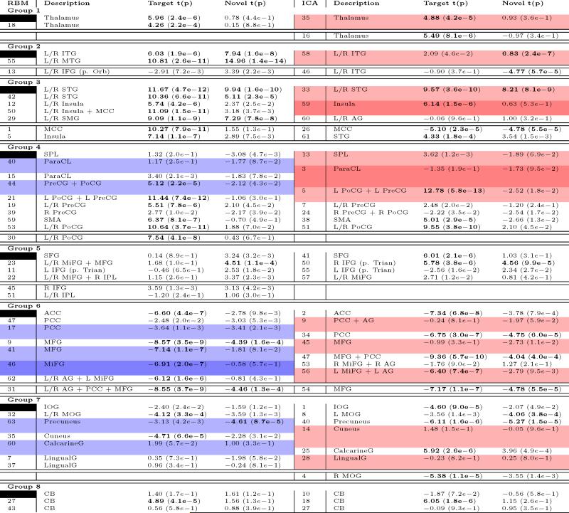
Table C.5: * Feature number, primary regions, t-values, and p-values to target and novel TC for RBM (left) and matched ICA (right) from a second-level t-test. Groupings of components (1-8) are determined from RBM modularity and are generally not consistent with ICA FNC modularity. For each group, white-shaded features above the double-line indicate a one-to-one match between RBM and ICA features with spatial correlation above 0:4. RBM features highlighted in blue correspond to multiple ICA features with spatial correlation above threshold. Similarly, ICA features highlighted in red correspond to multiple RBM features above threshold. Below the double-line in each group are RBM and ICA features with no corresponding feature.
 |
Footnotes
Publisher's Disclaimer: This is a PDF file of an unedited manuscript that has been accepted for publication. As a service to our customers we are providing this early version of the manuscript. The manuscript will undergo copyediting, typesetting, and review of the resulting proof before it is published in its final citable form. Please note that during the production process errors may be discovered which could affect the content, and all legal disclaimers that apply to the journal pertain.
References
- Abou-Elseoud A, Starck T, Remes J, Nikkinen J, Tervonen O, Kiviniemi V. The effect of model order selection in group PICA. Human Brain Mapping. 2010;31(8):1207–1216. doi: 10.1002/hbm.20929. [DOI] [PMC free article] [PubMed] [Google Scholar]
- Allen EA, Damaraju E, Plis SM, Erhardt EB, Eichele T, Calhoun VD. Tracking whole-brain connectivity dynamics in the resting state. Cerebral Cortex. 2012a doi: 10.1093/cercor/bhs352. [DOI] [PMC free article] [PubMed] [Google Scholar]
- Allen EA, Erhardt EB, Damaraju E, Gruner W, Segall JM, Silva RF, Havlicek M, Rachakonda S, Fries J, Kalyanam R, et al. A baseline for the multivariate comparison of resting-state networks. Frontiers in Systems Neuroscience. 2011;5(2) doi: 10.3389/fnsys.2011.00002. [DOI] [PMC free article] [PubMed] [Google Scholar]
- Allen EA, Erhardt EB, Wei Y, Eichele T, Calhoun VD. Capturing inter-subject variability with group independent component analysis of fMRI data: a simulation study. Neuroimage. 2012b;59(4):4141–4159. doi: 10.1016/j.neuroimage.2011.10.010. [DOI] [PMC free article] [PubMed] [Google Scholar]
- Beckmann CF, DeLuca M, Devlin JT, Smith SM. Investigations into resting-state connectivity using independent component analysis. Philosophical Transactions of the Royal Society B: Biological Sciences. 2005;360(1457):1001–1013. doi: 10.1098/rstb.2005.1634. [DOI] [PMC free article] [PubMed] [Google Scholar]
- Bell AJ, Sejnowski TJ. An informationmaximization approach to blind separation and blind deconvolution. Neural Computation. 1995;7 doi: 10.1162/neco.1995.7.6.1129. [DOI] [PubMed] [Google Scholar]
- Bengio Y, Courville AC, Vincent P. Unsupervised feature learning and deep learning: A review and new perspectives. Computing Research Repository. 2012 abs/1206.5538. [Google Scholar]
- Bengio Y, LeCunn Y. Large Scale Kernel Machines. MIT Press; 2007. Scaling learning algorithms towards AI. [Google Scholar]
- Biswal B, Zerrin Yetkin F, Haughton VM, Hyde JS. Functional connectivity in the motor cortex of resting human brain using echo-planar MRI. Magnetic Resonance in Medicine. 1995;34(4):537–541. doi: 10.1002/mrm.1910340409. [DOI] [PubMed] [Google Scholar]
- Burkard RE, Dell'Amico M, Martello S. Assignment problems. Siam. 2009 [Google Scholar]
- Calhoun VD, Adali T. Multi-subject independent component analysis of fMRI: A decade of intrinsic networks, default mode, and neurodiagnostic discovery. IEEE Reviews in Biomedical Engineering. 2012;5 doi: 10.1109/RBME.2012.2211076. [DOI] [PMC free article] [PubMed] [Google Scholar]
- Calhoun VD, Kiehl KA, Pearlson GD. Modulation of temporally coherent brain networks estimated using ICA at rest and during cognitive tasks. Human Brain Mapping. 2008;29 doi: 10.1002/hbm.20581. [DOI] [PMC free article] [PubMed] [Google Scholar]
- Calhoun VD, Sui J, Kiehl KA, Turner JA, Allen EA, Pearlson GD. Exploring the psychosis functional connectome: Aberrant intrinsic networks in schizophrenia and bipolar disorder. Frontiers in Neuropsychiatric Imaging and Stimulation. 2012;2 doi: 10.3389/fpsyt.2011.00075. [DOI] [PMC free article] [PubMed] [Google Scholar]
- Damoiseaux J, Rombouts S, Barkhof F, Scheltens P, Stam C, Smith SM, Beckmann C. Consistent resting-state networks across healthy subjects. Proceedings of the National Academy of Sciences. 2006;103(37):13848–13853. doi: 10.1073/pnas.0601417103. [DOI] [PMC free article] [PubMed] [Google Scholar]
- Erhardt E, Allen EA, Wei Y, Eichele T. SimTB, a simulation toolbox for fMRI data under a model of spatiotemporal separability. Neuroimage. 2012;59(4) doi: 10.1016/j.neuroimage.2011.11.088. [DOI] [PMC free article] [PubMed] [Google Scholar]
- Erhardt EB, Rachakonda S, Bedrick EJ, Allen EA, Adalh T, Calhoun VD. Comparison of multisubject ICA methods for analysis of fMRI data. Human Brain Mapping. 2011;32(12):2075–2095. doi: 10.1002/hbm.21170. [DOI] [PMC free article] [PubMed] [Google Scholar]
- Freudenburg ZV, Ramsey NF, Wronkeiwicz M, Smart WD, Pless R, Leuthardt EC. Real-time naive learning of neural correlates in ECoG electrophysiology. International Journal of Machine Learning and Computing. 2011 [Google Scholar]
- Glorot X, Border A, Bengio Y. Deep sparse rectifier neural networks. International Conference on Artificial Intelligence and Statistics. 2011 [Google Scholar]
- Goodfellow I, Courville A, Bengio Y. Large-scale feature learning with spike-and-slab sparse coding. arXiv preprint. 2012 arXiv:1206.6407. [Google Scholar]
- Hastie T, Friedman JH, Tibshirani R. Elements of Statistical Learning; Data Mining, Inference, and Prediction. Vol. 1. Springer; New York: 2001. [Google Scholar]
- Hinton G. Training products of experts by minimizing contrastive divergence. Neural Computation. 2000;14 doi: 10.1162/089976602760128018. [DOI] [PubMed] [Google Scholar]
- Hinton G. A practical guide to training restricted Boltzmann machines. Momentum. 2010;9(1) [Google Scholar]
- Hinton G, Osindero S. A fast learning algorithm for deep belief nets. Neural Computation. 2006;18 doi: 10.1162/neco.2006.18.7.1527. [DOI] [PubMed] [Google Scholar]
- Hinton G, Salakhutdinov R. Reducing the dimensionality of data with neural networks. Science. 2006 doi: 10.1126/science.1127647. [DOI] [PubMed] [Google Scholar]
- Kiviniemi V, Starck T, Remes J, Long X, Nikkinen J, Haapea M, Veijola J, Moilanen I, Isohanni M, Zang Y-F, et al. Functional segmentation of the brain cortex using high model order group PICA. Human Brain Mapping. 2009;30(12):3865–3886. doi: 10.1002/hbm.20813. [DOI] [PMC free article] [PubMed] [Google Scholar]
- Krizhevsky A, Sutskever I, Hinton G. Imagenet classification with deep convolutional neural networks. Neural Information Processing Systems. 2012 [Google Scholar]
- Laird AR, Eickhoff SB, Rottschy C, Bzdok D, Ray KL, Fox PT. Networks of task co-activations. NeuroImage. 2003 doi: 10.1016/j.neuroimage.2013.04.073. [DOI] [PMC free article] [PubMed] [Google Scholar]
- Lee QV, Monga R, Devin M, Chen K, Corrado GS, Dean J, Ng AY. Building high-level features using large scale unsupervised learning. International Conference on Machine Learning. 2012 [Google Scholar]
- Mohamed A, Dahl GE, Hinton G. Acoustic modeling using deep belief networks. IEEE transactions on audio, speech, and language processing. 2010 [Google Scholar]
- Nair V, Hinton G. Rectified linear units improve restricted Boltzmann machines. International Conference on Machine Learning. 2010 [Google Scholar]
- Ng AY. Feature selection, L1 vs. L2 regularization, and rotational invariance. International Conference on Machine Learning. 2004 [Google Scholar]
- Potluru VK, Plis SM, Jonathan L, Pearlmutter BA, Calhoun VD, Hayes TP. Block coordinate descent for sparse NMF. Proc. International Conference on Learning Representations. 2013 May; [Google Scholar]
- Rubinov M, Sporns O. Weight-conserving characterization of complex functional brain networks. Neuroimage. 2011;56(4):2068–2079. doi: 10.1016/j.neuroimage.2011.03.069. [DOI] [PubMed] [Google Scholar]
- Salakhutdinov R, Hinton G. Deep Boltzmann machines. International Conference on Machine Learning. 2009 [Google Scholar]
- Schmah T, Hinton GE, Zemel RS, Small SL, Strother SC. Generative versus discriminative training of rbms for classification of fMRI images. NIPS. 2008:1409–1416. [Google Scholar]
- Sjöstrand K. Informatics and Mathematical Modelling. Technical University of Denmark (DTU); 2005. Matlab implementation of lasso, lars, the elastic net and spca. [Google Scholar]
- Smith SM, Fox PT, Miller KL, Glahn DC, Fox PM, Mackay CE, Filippini N, Watkins KE, Toro R, Laird AR, et al. Correspondence of the brain's functional architecture during activation and rest. Proceedings of the National Academy of Sciences. 2009;106(31):13040–13045. doi: 10.1073/pnas.0905267106. [DOI] [PMC free article] [PubMed] [Google Scholar]
- Sorg C, Riedl V, Perneczky R, Kurz A, Wohlschlager AM. Impact of alzheimer's disease on the functional connectivity of spontaneous brain activity. Current Alzheimer Research. 2009;6 doi: 10.2174/156720509790147106. [DOI] [PubMed] [Google Scholar]
- Swanson N, Eichele T, Pearlson G, Kiehl K, Yu Q, Calhoun VD. Lateral differences in the default mode network in healthy controls and patients with schizophrenia. Human Brain Mapping. 2011;32(4):654–664. doi: 10.1002/hbm.21055. [DOI] [PMC free article] [PubMed] [Google Scholar]
- van Gerven MA, de Lange FP, Heskes T. Neural decoding with hierarchical generative models. Neural Computation. 2010;22(12):3127–3142. doi: 10.1162/NECO_a_00047. [DOI] [PubMed] [Google Scholar]
- Varoquaux G, Gramfort A, Pedregosa F, Michel V, Thirion B. In: Information Processing in Medical Imaging. Springer; 2011. Multi-subject dictionary learning to segment an atlas of brain spontaneous activity. pp. 562–573. [DOI] [PubMed] [Google Scholar]
- Zou H, Hastie T, Tibshirani R. Sparse principal component analysis. Journal of Computational and Graphical Statistics. 2006;15(2):265–286. [Google Scholar]
- Zuo X-N, Kelly C, Adelstein JS, Klein DF, Castellanos FX, Milham MP. Reliable intrinsic connectivity networks: test-retest evaluation using ICA and dual regression approach. Neuroimage. 2010;49(3):2163–2177. doi: 10.1016/j.neuroimage.2009.10.080. [DOI] [PMC free article] [PubMed] [Google Scholar]