Setting Up the JBrowse Genome Browser

Abstract

JBrowse is a web-based tool for visualizing genomic data. Unlike most other web-based genome browsers, JBrowse exploits the capabilities of the user's web browser to make scrolling and zooming fast and smooth. It supports the browsers used by almost all internet users, and is relatively simple to install. JBrowse can utilize multiple types of data in a variety of common genomic data formats, including genomic feature data in bioperl databases, GFF files, and BED files, and quantitative data in wiggle files. This unit describes how to obtain the JBrowse software, set it up on a Linux or Mac OS X computer running as a web server and incorporate genome annotation data from multiple sources into JBrowse. After completing the protocols described in this unit, the reader will have a web site that other users can visit to browse the genomic data.

INTRODUCTION

JBrowse (Skinner et al. 2009) is a compact and easily-installed software package for the web-based browsing of genomes and genome annotations.

Like other genome browsers, such as the UCSC browser (Unit 1.4; Kent et al. 2002) or GBrowse (Unit 9.9; Stein et al. 2002), JBrowse enables the user to visualize discrete features and gene structures alongside quantitative information. Unlike other web-based genome browsers, with JBrowse, the web browser (e.g., Firefox, Internet explorer, Safari, etc.) does most of the work; this allows the user to interact with the data without having to wait for the server to respond. This approach of moving work from the web server to the web browser makes JBrowse simpler to set up and maintain than other browsers, while being faster and easier to utilize due to the use of advanced client-side user interface enhancements. JBrowse is part of the Generic Model Organism Database (GMOD) project (www.gmod.org), a suite of tools for generating and maintaining genomic databases. Like the other tools in GMOD project (of which it is a part), JBrowse is a piece of software that you install yourself and use with your own data. This is in contrast to services such as the UCSC genome browser (Unit 1.4; Kent et al. 2002) or the Ensembl genome browser (Unit 1.15; Hubbard et al. 2007), which focus mainly on hosting the most-in-demand genomes with rather more limited scope for adding your own data.

Each of the protocols here describes a different way of setting up a JBrowse instance. Such an “instance” is a copy of the JBrowse software combined with genomic data for an organism, placed on a server so that an end user can visit the site in their web browser and browse a genome. Basic Protocol 1 describes setting up a JBrowse instance for genome annotations stored in the common FASTA, GFF3, and/or BED formats. Alternate Protocol 1 describes an alternate way to set up JBrowse, for genome annotations that are stored in a relational database. Alternate Protocol 2 describes the process of setting up a JBrowse instance from a Genbank record. Support Protocol 1 describes the initial installation process for JBrowse and its dependencies.

BASIC PROTOCOL 1

SETTING UP A JBROWSE INSTANCE USING FLATFILES AS A DATA SOURCE

This protocol will walk through the installation of JBrowse and setup process, assuming that the user has already successfully completed the installation steps in Support Protocol 1.

In JBrowse, software running in the web browser downloads specially-formatted data files from the server and displays a visual representation of them. The process of setting up a JBrowse instance involves running the programs that come with JBrowse to generate those specially-formatted data files from some data source.

After JBrowse is downloaded and installed (see Support Protocol 1), the JBrowse directory contains a file named “index.html”. This file is the main HTML front-end to JBrowse, and will (eventually) be displayed in the end user's web browser (e.g. Firefox). However, before it is ready to do this, the user will need to add some genomic data.

JBrowse supports a variety of data sources; it uses the same underlying BioPerl machinery as the GBrowse genome browser, and therefore supports all of the same data sources. In addition to genomic databases (described in Alternate Protocol 1), JBrowse supports several flat-file formats, including FASTA (Appendix 1B) for reference sequence data and GFF3 and BED for genomic feature data.

Broadly speaking, the GFF3 and BED formats are used to store similar data--mainly, the boundaries of genomic features such as genes (for example, a line in a GFF3 or BED file might describe the gene TP53 and state that it is found on chromosome 17 from bases 7,571,720 to 7,590,863). Beyond such basic feature information, though, the two formats differ; GFF3 files can contain richer information about each feature, and can describe multi-level feature hierarchies (e.g., a gene feature being the parent of a transcript feature, which itself is the parent of several exon, intron, and CDS or UTR features). BED, on the other hand, is simpler and more limited in the kinds of data it can store and the depth of the feature hierarchies. Both formats are commonly used to store and communicate genomic feature information. JBrowse can use either one, or both.

Each feature in the GFF3 format consists of a line of text, containing several columns separated by tab characters; here are a few lines from the example GFF3 file included with JBrowse:

ctgA	example remark	13280	16394	.	+	.	Name=f08
ctgA	example remark	15329	15533	.	+	.	Name=f10

A brief description of the GFF3 columns is shown in Table 9.13.1; for full details refer to the specification: http://www.sequenceontology.org/gff3.shtml.

Table 9.13.1.

Description of columns in GFF3 format

Column	Description
Reference sequence name	Name of the sequence that the feature is defined on (commonly a chromosome or contig)
Source	The source of the feature. For features that were generated by software, this is commonly the name of the software; for human-curated features, this is commonly the name of the group performing the curation (e.g., a model organism database)
Type	The type of the feature from the Sequence Ontology (http://www.sequenceontology.org/)
Start	The start position of the feature
End	The end position of the feature
Score	(optional) The score of the feature
Strand	(optional) The strand on which the feature occurs
Phase	(optional) The phase of the feature (e.g., for CDS features, indicates that the first full codon in the feature starts this many bases after the start of the feature)
Attributes	(optional) A set of name=value pairs specifying information not contained within the other GFF columns (often contains Name and ID information)

The BED format is an alternative to GFF3. The BED format also represents each feature by a line containing tab-separated columns. Here are a few example lines:

ctgA	1659	1984	f07	.	+
ctgA	3014	6130	f06	.	+
ctgA	4715	5968	f05	.	-
ctgA	13280	16394	f08	.	+
ctgA	15329	15533	f10	.	+

The columns of the BED format are briefly described in Table 9.13.2. For full details, refer to the format FAQ from UC Santa Cruz: http://genome.ucsc.edu/FAQ/FAQformat.html.

Table 9.13.2.

Description of columns in BED format

Reference sequence name	Name of the chromosome or scaffold
Start	Start position of the feature
End	End position of the feature
Name	(optional) Name of the feature
Score	(optional) Score of the feature
Strand	(optional) Strand on which the feature is defined
Thick Start	(optional) Position where the feature should be drawn thickly (e.g., for transcript models, the start of the coding sequence)
Thick End	(optional) Position where the feature should no longer be drawn thickly (e.g., for transcript models, the end of the coding sequence)
Item Rgb	(optional) Color to use to draw the feature
Block Count	(optional) Number of blocks (e.g., for transcript models, the number of exons)
Block Sizes	(optional) Sizes of blocks (e.g., for transcript models, the size of each exon)
Block Starts	(optional) Start points of blocks (e.g., for transcript models, the starting point of each exon)

This protocol utilizes the term “user” to describe the person installing JBrowse and importing data into a JBrowse instance; the phrase “end user” will describe the person who visits that JBrowse instance in their web browser. In this protocol, the user will set up an instance of JBrowse using the included example data. The tutorial example refers to the “volvox” genome, but the sequence and all annotation data is simulated and does not correspond to volvox or any other living organism.

Necessary Resources

Hardware

• Linux or Mac OS X machine

• RAM – roughly 512 megabytes; more for large data sets

• Internet connection

Software

• Installation of all necessary software is described in Support Protocol 1.

1. Import reference sequence data into the JBrowse instance. To do this, first open a terminal window, go into the JBrowse directory, and then run the prepare-refseqs.pl program from the command line (the “$” symbol represents the Unix shell prompt).

   • $ cd <JBrowse directory>
   • $ bin/prepare-refseqs.pl --fasta docs/tutorial/data_files/volvox.fa

   Where <JBrowse directory> is the directory created in Support Protocol 1; commonly /var/www/html/jbrowse (on Red Hat/CentOS/Fedora machines), /var/www/jbrowse (on Ubuntu), or /Library/WebServer/Documents/jbrowse (on OS X).

   If an end user visits the JBrowse instance now, they should see the JBrowse UI (user interface) elements: buttons for zooming and scrolling, a drop-down box for selecting a reference sequence, and a box showing the current genomic location being viewed. If the end user zooms in all the way, they should see DNA sequence data (Figure 9.13.1).

   To see this, load or reload the “index.html” page in your browser.

2. It is now time to add some genomic feature tracks. Run bin/flatfile-to-json.pl to add the gene track:

   • $ bin/flatfile-to-json.pl --tracklabel gene --key “Gene” --gff docs/tutorial/data_files/volvox.gff3 --cssclass feature2 --getLabel --type gene --autocomplete all

   This step uses the command-line arguments shown in Table 9.13.3. Note that this example command wraps across several lines, but should be entered as a single line. You may use the backslash (“\”) character to continue the command across several lines.

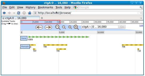
   If an end user visits the JBrowse instance in their web browser, then they'll see a new track as shown in Figure 9.13.2.

   In JBrowse, genomic feature data is organized into tracks, which usually contain features of the same or similar types. For example, there might be a “transcript” track, an “EST” track, and a “SNP” track. JBrowse's bin/flatfile-to-json.pl program takes as input a file with genomic feature data and also takes some command-line arguments that specify how to process the file, and uses those inputs to generate JBrowse's data files for one track. If the user wants to create multiple tracks, they can run the program multiple times and specify different settings each time.

3. Run bin/flatfile-to-json.pl again, with different arguments, to create a new track from a BED file (Figure 9.13.3):

   • $ bin/flatfile-to-json.pl --bed docs/tutorial/data_files/volvox-remark.bed --tracklabel remark --key “Remark” --cssclass feature3 --getLabel --autocomplete label
4. 4. Add a quantitative track using bin/wig-to-json.pl (Figure 9.13.4):

   • $ bin/wig-to-json.pl --wig
   • docs/tutorial/data_files/volvox_microarray.wig --tracklabel
   • wiggle_example --key “20 degrees, 2 hr”

   JBrowse also supports visualizing quantitative data in the “wiggle” format. This type of data is useful for dense quantitative data like transcription level data (e.g., from microarrays or RNA-seq). If you have data with a numeric value at a series of genomic locations, that data can be put into a wiggle file. The genomic locations can be specified in a few different ways as described at http://genome.ucsc.edu/goldenPath/help/wiggle.html, but the wiggle file used in this protocol is in the simplest format. Here are a few lines from the example wiggle file included with JBrowse; the first line specifies that this file contains data points that are separated by a fixed distance (indicated below by “fixedStep”); the data points are 100 bases wide (indicated by “span=100”), starting at base 1 (indicated by “start=1”) and occurring every 100 bases thereafter (indicated by “step=100”):

   fixedStep chrom=ctgA start=1 step=100 span=100

   281

   183

   213

   191

   288And this is how the result looks:

5. Run the bin/generate-names.pl program to enable the end user to search for feature names or identifiers:

   • $ bin/generate-names.pl

   This step enables end users to search for specific features by name. Earlier in this protocol the –autocomplete option passed to flatfile-to-json.pl caused this program to generate lists of feature names (in addition to the locations of the associated features) and place them in separate track files. The generate-names.pl program takes all of the separate per-track lists of names, collects them together, and generates another set of specially-formatted files. Those files allow the web browser to search for a specific feature name or ID. If generate-names.pl generates no error messages, that means the program has completed successfully. If an end user visits the page now, enters a feature name (e.g., “f05”) into the text box that shows the current genomic location, and clicks “Go”, they'll be taken to that feature.

Figure 9.13.1.

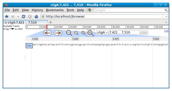
JBrowse instance with just DNA sequence track, zoomed in to the individual base level.

Table 9.13.3.

Description of command-line arguments used with the gene track

Argument	Required	Purpose
--tracklabel	Yes	Unique identifier for the track
--key	Yes	Human-readable label for the track
--gff or --gff2 or --bed	Yes	Path to input flat file
--cssclass	No	Describes how the features should look
--getLabel	No	Include feature labels in the output
--type	No	Only process features of the given type
--autocomplete	No	Make it possible to search for features in this track

Figure 9.13.2.

Screenshot of JBrowse with newly-created “gene” track.

Figure 9.13.3.

Screenshot of JBrowse instance with newly-created “Remark” track.

Figure 9.13.4.

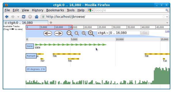
Screenshot of JBrowse instance with newly-created quantitative track.

ALTERNATE PROTOCOL 1

SETTING UP A JBROWSE INSTANCE USING A RELATIONAL DATABASE AS THE DATA SOURCE

JBrowse can also access data in any of the databases that work with the BioPerl Bio::DB API. Two common database schemas that support that API are the chado schema and the Bio::DB::SeqFeature::Store schema. This protocol describes using JBrowse with Bio::DB::SeqFeature::Store and the MySQL database server.

Necessary Resources

Hardware

• Linux or Mac OS X machine

• RAM – roughly 512 megabytes; more for large data sets

• Internet connection

Software

• Installation of all necessary software is described in Support Protocol 1.

1. Create the database using the mysql command-line tool:

   • $ mysql -u root

   mysql> create database jbrowse_example;

   Query OK, 1 row affected (0.00 sec)

   mysql> grant all on jbrowse_example.* to "@'localhost';

   Query OK, 0 rows affected (0.00 sec)

2. Load the database using BioPerl's bp_seqfeature_load.pl script

   • $ bp_seqfeature_load.pl –dsn=dbi:mysql:jbrowse_example --
   • adaptor=DBI::mysql --fast --create docs/tutorial/data_files/volvox.fa
   • docs/tutorial/data_files/volvox.gff3

   In Basic Protocol 1, the user runs the bin/flatfile-to-json.pl program once per track. This protocol, by contrast, uses one program that generates multiple tracks from a data source. The detailed settings for each track (supplied as command-line arguments in Basic Protocol 1) are instead specified in a configuration file. This configuration file is helpful if the user runs the JBrowse programs repeatedly (for example, if the data source is updated with new data) then the configuration file is a convenient place to store those track-specific settings.

   The JBrowse distribution includes an example configuration file; however, it needs to be adjusted to work with the database that the user created in steps 1 and 2 of this protocol (see step 3).

3. Edit the example configuration file. Find the “db_args” setting and change it from:

   “db_args”: { “-adaptor”: “memory”,

    “-dir”: “docs/tutorial/data_files” },

   To:

   “db_args”: { “-adaptor”: “DBI::mysql”,

   “-dsn”: “dbi:mysql:jbrowse_example” },

   This tells JBrowse that the database is a MySQL database, and, of the mysql databases on the machine, to use the one called “jbrowse_example”.

   Most of the remaining of the file contains the per-track settings. These mostly correspond to the command-line parameters used with the flatfile-to-json.pl program described in Basic Protocol 1 (Table 9.13.3).

4. As in Basic Protocol 1, use the prepare-refseqs.pl program to import reference sequence data into this JBrowse instance:

   • $ bin/prepare-refseqs.pl --conf docs/tutorial/conf_files/volvox.json --refs ctgA
   • This performs the same function that this program served in Basic Protocol 1, but uses different command-line arguments. The --conf command-line argument specifies the configuration file; the --refs command line argument gives the names of the reference sequences in the format of a comma-separated list (for example, if there was a second contig named “ctgB”, the --refs argument would then be ctgA,ctgB).
5. Run bin/biodb-to-json.pl to extract data from the database and add it to this JBrowse instance.

   • $ bin/biodb-to-json.pl --conf docs/tutorial/conf_files/volvox.json
6. Run generate-names.pl to enable name/ID searching:

   • $ bin/generate-names.pl

ALTERNATE PROTOCOL 2

SETTING UP A JBROWSE INSTANCE USING NCBI GENBANK FILES AS A DATA SOURCE

JBrowse does not directly support files in genbank formats, but a bioperl conversion program can take genbank files and create GFF3 files that JBrowse can process. This protocol walks through the process of taking a genbank file, converting it into GFF3, and incorporating it into a JBrowse instance.

Necessary Resources

Hardware

• Linux or Mac OS X machine

• RAM – roughly 512 megabytes; more for large data sets

• Internet connection

Software

• Installation of all necessary software is described in Support Protocol 1.

Files

• From

  • ftp://ftp.ncbi.nih.gov/genomes/Saccharomyces_cerevisiae/CHR_I/
• download the file:

  • NC_001133.gbk

  NOTE: Data can be imported into JBrowse from GenBank .gbk files, by converting those files into GFF3 with scripts from BioPerl.

1. Use the BioPerl bp_genbank2gff3.pl script to generate a GFF3 file:

   • $ bp_genbank2gff3.pl NC_001133.gbk
2. Edit the generated file, named NC_001133.gbk.gff, and change this line:

   • # sequence-region NC_001133 1 230208
   • to the following:

     • ##sequence-region NC_001133 1 230208
     • This corrects a small bug in the bp_genbank2gff3.pl script.
3. Go into the JBrowse directory and use bin/prepare-refseqs.pl to initialize the JBrowse instance. JBrowse comes with a suitable configuration file (named yeast_genbank.json) in the docs/examples/config directory:

   • $ bin/prepare-refseqs.pl --conf docs/examples/config/yeast_genbank.json --refs NC_001133
4. Use bin/biodb-to-json.pl to populate the tracks:

   • $ bin/biodb-to-json.pl --conf docs/examples/config/yeast_genbank.json
5. Make the features searchable with bin/generate-names.pl:

   • $ bin/generate-names.pl

SUPPORT PROTOCOL 1

DOWNLOADING/INSTALLING JBROWSE

The protocol describes how to obtain and install the JBrowse software and its prerequisites. After performing the steps in this protocol, the user should be able to go on to Basic Protocol 1, or Alternate Protocols 1 or 2.

Necessary Resources

Hardware

• Linux or Mac OS X machine

• RAM – roughly 512 megabytes; more for large data sets

• Internet connection

1. Install perl and related packages. These are usually available from your operating system provider; the way to install them depends on your operating system. This protocol describes how to install the necessary software on the Red Hat, CentOS, Fedora, and Ubuntu flavors of Linux, and on Apple's Mac OS X operating system.

   • Red Hat/CentOS/fedora:

     • $ sudo yum install perl
   • Ubuntu:

     • $ sudo apt-get install perl
   • OS X:

     • You don't need to do anything on OSX; Perl is installed by default.
2. For quantitative tracks, you need to install a C++ compiler program, the ‘make’ program, the ‘libpng’ library, and the libpng header files. As with Perl, these are usually provided by your operating system provider:

   • Red Hat/CentOS/fedora:

     • $ sudo yum install gcc-c++ make libpng libpng-devel
   • Ubuntu:

     • $ sudo apt-get install g++ make libpng12-0 libpng12-dev
   • OS X:

     • For the C++ compiler and ‘make’ program, you need to install XCode tools, either using the install CD/DVD that came with your computer, or by downloading them directly from Apple at http://developer.apple.com/.

   The ‘libpng.dylib’ library file and ‘png.h’ header file should already be installed in directories /usr/X11R6/lib and /usr/X11R6/include, respectively.

3. Install the necessary perl modules from CPAN:

   • $ sudo cpan
   • cpan> install CJFIELDS/BioPerl-1.6.1.tar.gz JSON JSON::XS
4. For Alternate Protocol 1, install MySQL:

   • Red Hat/CentOS/fedora:

     • $ sudo yum install mysql perl-DBD-MySQL
   • Ubuntu:

     • $ sudo apt-get install mysql-server libdbd-mysql-perl
   • OS X:

     • There are multiple ways of installing MySQL on OS X; the easiest is to go to the MySQL Downloads website (http://dev.mysql.com/downloads/mysql/) and download a ‘.dmg’ (disk image) file containing the MySQL server.

5. Download a zipfile from github, containing the JBrowse source code. You can do this by pointing your web browser at: http://github.com/jbrowse/jbrowse/zipball/master.

   Alternatively, you can download the zipfile directly from the command line, using the ‘wget’ utility, if it is installed on your system:

   $ wget http://github.com/jbrowse/jbrowse/zipball/master

6. Uncompress the zip file downloaded in the previous step

   • $ unzip jbrowse*.zip
7. Build the quantitative track (wiggle) renderer:

   • Red Hat/CentOS/Fedora/Ubuntu:

     • $ cd jbrowse*
     • $ ./configure
     • $ make
   • OS X:

     • $ cd jbrowse*
     • $ ./configure
     • $ make GCC_LIB_ARGS=-L/usr/X11R6/lib GCC_INC_ARGS=-I/usr/X11R6/include
8. Move the JBrowse directory to where it will be served by the web server:

   • Red Hat/CentOS/fedora:

     • $ cd ..
     • $ sudo mv jbrowse*/ /var/www/html/jbrowse
   • Ubuntu:

     • $ cd ..
     • $ sudo mv jbrowse*/ /var/www/jbrowse
   • OS X:

     • $ cd ..
     • $ sudo mv jbrowse*/ /Library/WebServer/Documents/jbrowse

9. To check that the JBrowse instance is accessible, go to http://localhost/jbrowse in your web browser. You should see a completely blank page; this page will be populated when you add a genome sequence and tracks as described in Basic Protocol 1.

GUIDELINES FOR UNDERSTANDING RESULTS

The results of running each major step of Basic Protocol 1 can be seen in the figures referenced within that section. After completing Support Protocol 1, and after each major step of Basic Protocol 1, a web browser can be pointed at the URL corresponding to the jbrowse installation, providing immediate feedback on the success or failure of that step:

1. Following installation (Support Protocol 1), a web browser pointing at the appropriate URL (typically http://localhost/jbrowse) should display a blank page. Some JavaScript errors may be displayed in the console. If, instead of a blank page, you get an error such as “403 Forbidden” or “404 Not Found”, then there may problems with your installation (see Troubleshooting).

2. After adding the sequence data, reloading the web page should yield a view similar to that shown in Figure 9.13.1.

3. After adding a gene annotation track, and successive annotation tracks, reloading the web page should yield a view similar to that shown in Figures 9.13.2 and 9.13.3.

After adding a quantitative (Wiggle) track, reloading the web page should yield a view similar to that shown in Figure 9.13.4.

Problems, and potential resolutions to those problems, are described below in the “Troubleshooting” section.

COMMENTARY

Background Information

A variety of web-based genome browsers have existed for several years. Those systems generally have database engines running on the web server alongside a body of genome-browser software. When a user visits a genome browser page, that software queries the database and draws a picture of a genomic region and sends that picture to the web browser, which just displays it.

Over the last ten years, however, many software systems have begun to shift work away from the web server and onto the user's web browser. Having part of the application running on the user's machine allows for much richer interaction between the user and the application. It also reduces the amount of work that the server must do, which reduces or eliminates the time users have to spend waiting for the server to respond.

JBrowse is an example of this shift; it does part of the work on the server but moves the bulk of the work to the user's web browser. The initial server-side work that JBrowse does (getting data from some data source) is almost the same as the first part of what GBrowse (Unit 9.9) does. In fact, JBrowse uses many of the same software components for data access that were built for the GBrowse genome browser. This sharing and reuse of software is one of the ways that JBrowse builds on the work done for GBrowse, and it means that JBrowse is compatible with the same set of data sources as GBrowse.

The next step differs, however, instead of using that data to draw a picture on the server, JBrowse uses it to create files on the server that the web browser downloads and uses to present a graphical representation of a region of a genome. In addition to the advantages listed above, this approach simplifies the server environment, which helps make JBrowse simple to set up. When a user visits a JBrowse instance, the server does not have to run any JBrowse software; it just sends the files that were created in advance by the JBrowse programs. Many web hosting environments enable users to put such static files online, but restrict the user's ability to install and run software. JBrowse can be used in those environments; all the user has to do is install and run JBrowse on their own computer and then upload the resulting JBrowse instance to the server.

The main (“master”) version of JBrowse currently handles tracks with tens of thousands of features per reference sequence, but does not deal well with tracks like human EST or SNP tracks with millions of features. The version currently in development handles tracks of this size by downloading regions only when they are needed; as of this writing the largest tracks tested with the development version of JBrowse have contained next-generation sequencing read data with tens of millions of features per reference sequence.

Critical Parameters and Troubleshooting

If you encounter problems with JBrowse, the best thing to do is to consult the email list, first by searching the archive here: http://gmod.827538.n3.nabble.com/JBrowse-f815920.html.

And then, if you don't see any messages that solve your problem, send a message to the list at gmod-ajax@sourceforge.net.

Common problems that users encounter include:

1. The JBrowse programs fail with an error message -- there are multiple reasons why this can happen; the main ones are:

   1. Running programs from outside of the JBrowse directory -- JBrowse works best if the programs are run from within the JBrowse directory (the directory that contains the index.html file) as shown above.
   2. Missing or outdated dependencies -- Some JBrowse programs use parts of BioPerl in which bugs have recently been fixed. Using the latest available stable version of BioPerl (1.6.1 as of this writing) will help avoid problems.
2. When a user visits a JBrowse instance in their web browser, they get a 403 (Forbidden) error -- This can arise as a result of restrictive permissions in the JBrowse directory; to fix it, try going into the JBrowse directory and changing the permissions of all files so as to be readable by Unix users other than yourself, as follows:

   • $ chmod −R o+r .

3. Subfeatures not showing up -- Subfeatures (such as exons in a transcript) are, by default, not included in the files that JBrowse generates. To include them, specify --getSubs (for flatfile-to-json.pl) or “subfeatures”: true in the config file (for biodb-to-json.pl).

APPENDIX 1B

Common File Formats

This appendix discusses a few of the file formats frequently encountered in bioinformatics.

FASTA FILES

FASTA files may contain DNA, RNA, or protein sequences. In each case, the sequence is written in the standard IUPAC single-letter codes (APPENDIX 1A), with the following exceptions:

• Lowercase letters are accepted;

• A hyphen (−) represents a gap of indeterminate length;

• The letter U represents selenocysteine in protein sequences;

• An asterisk (*) in a protein sequence indicates a translation stop.

A FASTA file may contain one or more sequences. A file with multiple sequences is called a multi-FASTA file. The first line, or descriptor line (see discussion below), of each new entry begins with a greater-than sign (>), followed by a single-line description of the sequence that follows. This title line may be any length, including simply the greater-than sign followed by no additional characters. Subsequent lines contain the sequence (Fig. A.1B.1). It is recommended that sequence lines be less than 80 characters.

NCBI Descriptor Lines

In typical NCBI descriptor lines, pipe (“|”) characters delineate key fields. For example:

• >gi|532319|pir|TVFV2E|TVFV2E envelope protein

The syntax of NCBI sequence FASTA format descriptor lines depends on the database from which each sequence was obtained. Table A.1B.1 lists the identifiers for the databases from which the sequences were derived.

“gi” identifiers are being assigned by NCBI for all sequences contained within NCBI's sequence databases. The “gi” identifier provides a uniform and stable naming convention whereby a specific sequence is assigned its unique gi identifier. If a nucleotide or protein sequence changes, however, a new gi identifier is assigned, even if the accession number of the record remains unchanged. Thus gi identifiers provide a mechanism for identifying the exact sequence that was used or retrieved in a given search.

Figure A.1B.1.

A sample FASTA file that contains the sequences for two homologous proteins, actophorin and yeast cofilin. Note that a greater-than sign (>) designates the beginning of each entry and that each of the lines of sequence contains less than 80 characters.

Table A.1B.1.

Identifiers to be Used With Sequence Databases

Database name	Identifier syntax
GenBank	gb|accession|locus
EMBL Data Library	emb|accession|locus
DDBJ (DNA Database of Japan)	dbj|accession|locus
NBRF PIR	pir||entry
Protein Research Foundation	prf||name
SWISS-PROT	sp|accession|entry name
Brookhaven Protein Data Bank	pdb|entry|chain
Patents	pat|country|number
GenInfo Backbone identifier	bbs|number
General database identifier	gnl|database|identifier
NCBI Reference Sequence	ref|accession|locus
Local sequence identifier	lcl|identifier

In the example above, 532319 is the gi accession number, TVFV2E is the PIR accession code, and TVFV2E envelope protein is the description of the sequence. Note that in this case there are two accession codes (a gi number and a PIR code).

The gnl (“general”) identifier allows databases not on the above list to be identified with the same syntax. An example here is the PID identifier:

• gnl|PID|e1632

PID stands for Protein ID; the e (in e1632) indicates that this ID was issued by EMBL. The pipe (“|”) separates different fields as listed in the above table. In some cases, a field is left empty, even though the original specification called for including this field. To make these identifiers backwardly compatible for software applications that expect these fields, the empty field is denoted by an additional pipe (“||”).

GenBank FLAT FILES

GenBank Files summarize pertinent information (e.g., sequence, size, source organism, and key references) for genes and gene products. They are readily available from the NCBI server (http://www.ncbi.nlm.nih.gov). Each file is broken into fields that designate what information is found on the following line(s). New fields are identified by a left-justified field name (given in capital letters) at the beginning of a new line of text. Some fields contain subfields, which are indented on subsequent lines. Table A.1B.2 lists the possible field names and describes the contents of each field. It is important to note that any given GenBank file may not contain every field. Figure A.1B.2 illustrates one example of a GenBank file. Additional information regarding the content and format of GenBank records may be found at http://www.ncbi.nlm.nih.gov/Sitemap/samplerecord.html.

If you are creating a sequence file in GenBank format, it may contain multiple sequences. Each new sequence begins with a LOCUS field. The other fields are optional, except for the ORIGIN field, which marks the beginning of the sequence. Two slashes (//) mark the end of the sequence (Fig. A.1B.2).

Table A.1B.2.

A Summary of Fields Commonly Found in GenBank Records (Fig. A.1B.2)

Field	Identifier(s) in Figure A.1B.2	Contents
LOCUS	1a: Locus name	Although the locus name was originally intended to identify similar sequences, it no longer carries such significance. Each GenBank file has a unique locus name. Often, it is either the first letter of the genus and species followed by the accession number, or simply the GenBank accession number of the file.
	1b: Sequence length	The number of nucleotide base pairs (bp) or amino acid residues (aa) in the gene or gene product.
	1c: Molecule type	Identifies the type of sequence found in a particular file. Possibilities include: genomic DNA, genomic RNA, precursor RNA, mRNA, rRNA, tRNA, small nuclear RNA, and cytoplasmic RNA.
	1d: Molecular topology	The molecule's expected topology. The options are linear and circular.
	1e: GenBank division	Each GenBank sequence is currently classified in one of the following 17 subdivisions: PRI, primates; ROD, rodents; MAM, mammals (excluding primates and rodents); VRT, vertebrates (excluding mammals); INV, invertebrates; PLN, plants, fungi, and algae; BCT, bacteria; VRL, viral; PHG, bacteriophages; SYN, synthetic; UNA, unannotated; EST, expressed sequence tag; PAT, patent sequence; STS, sequence tagged sites; GSS, genome survey sequence; HTG, high-throughput genomic sequence; HTC, unfinished high-throughput cDNA sequence. Note that the organismal subdivisions do not coincide with the current NCBI taxonomy. They are purely historical.
	1f: Modification date	Indicates when the file was last revised.
DEFINITION	2	A brief description of the sequence, including the organism source and the gene or protein name.
ACCESSION	3	A unique, stable, identifier for the particular file, which is usually a combination of one or two letters with five or six digits.
VERSION	4	Allows users to track multiple incarnations of a given sequence. The version number is the accession number concatenated with a period and a number. For the first version of a particular accession, the number following the period is set to 1. Each time the sequence data are modified, the number following the period is incremented by 1. The example shown in Figure A.1B.2 is the first version of accession number M93361.
		This field will also contain a GenInfo Identifier (GI) for nucleotide sequence files. This number uniquely identifies each nucleotide sequence in GenBank, even if they differ by a single nucleotide. Note that, unlike the accession number for a file, the GI number may change.
KEYWORDS	5	A word or phrase describing the sequence. Although frequently found in older GenBank records, this field is generally not present in more recent GenBank files.
SOURCE	6	The first line is a free-format description of the source organism, followed by the molecule type. The subsequent lines contain the subfield ORGANISM, which has the complete scientific name of the source organism and its phylogenetic classification as given by the NCBI Taxonomy Database.
REFERENCE	7	Publications by the authors of the GenBank entry that discuss the molecule. Multiple publications may be listed in chronological order, ending with the most recent. Each reference entry will contain subfields (e.g., AUTHORS, TITLE, JOURNAL, MEDLINE) that are appropriate for the particular publication type.
FEATURES	8	This is essentially a concise summary of the gene or protein annotation. It offers a list of genes, gene products, and regions of biological interest that have been identified within the reported sequence. The first subfield in each FEATURE list is the source subfield, which contains the length of the sequence, the scientific name of the source organism, and the taxon ID number. Additional subfields are given—e.g., gene, promoter, TATA signal, 5′ UTR, 3′ UTR, and coding sequence (CDS)—depending on the features within the sequence. For each feature, the GenBank record provides its location within the sequence and other pertinent information (e.g., the product or gene name, possible function, and protein translation).
BASE COUNT	9	The number of adenine, cytosine, thymine (or uracil), and guanine nucleotide bases within the sequence.
ORIGIN	10	This field is often left blank. In older records, it may contain the experimentally derived restriction cleavage site. Note that the ORIGIN field should be included in every GenBank record, even if it contains no information. Most parsers look for the sequence on the first line after the word ORIGIN.
	11	The sequence data with 60 bases (or residues) per line. The bases on each line are presented in six groups of ten bases per group, with the groups separated by spaces. The sequence ends with two slashes (//).

PHYLIP FILES

The Phylogeny Inference Package (PHYLIP) is a suite of programs used to infer phylogenies and generate evolutionary trees. The PHYLIP package allows users to generate distance matrices and apply a variety of phylogenetic methods to both nucleotide and protein sequences.

All of the programs in the package that use sequence data as the input (usually the result of a multiple sequence alignment) require that the sequences be formatted in PHYLIP's own “PHYLIP format.” An example of a PHYLIP-formatted file is shown in Figure A.1B.3. The file begins with a line containing two numbers; the first number represents the number of sequences in the data set (here, 5), and the second number represents the length of the alignment (here, 547 amino acids). The five sequences then follow, in “interleaved” format; this is different from the “sequential” FASTA format described above, where a sequence is listed in its entirety before the next sequence begins. In the first block, each sequence is preceded by an identifier that can be up to ten characters in length.

Figure A.1B.2.

A sample GenBank record. Circled numbers identify the fields listed in Table A.1B.1.

PHYLIP files usually take the file extension .phy.

MSF FILES

Multiple sequence files (called “MSF files”) are used by the individual programs within the GCG (Wisconsin) sequence analysis package. The GCG suite (UNIT 3.6) provides a large number of programs designed for sequence comparison, the generation of multiple sequence alignments, gene and secondary structure prediction, and pattern recognition, to name a few.

As with PHYLIP, the programs in the GCG package that use multiple sequence alignment data as the input require that the sequences be provided in MSF format. An example of an MSF-formatted file is shown in Figure A.1B.4. All MSF files begin with either PileUp, !!NA MULTIPLE ALIGNMENT, or !!AA MULTIPLE ALIGNMENT on the first line of the file. In the line that begins with MSF:, the length of the alignment is given (here, 547 amino acids), followed by the type of alignment (N for nucleotide, P for protein), a checksum number, and two dots, which signify the end of the descriptive header. The next block of lines contains information on the sequences in the alignment, giving their name, length, a checksum, and weight. A double slash then precedes the sequences, which are shown in interleaved format.

Figure A.1B.3.

A sample PHYLIP-formatted file. The five sequences shown are HIV-1 and HIV-2 gag proteins from a variety of isolates. See text for details.

Figure A.1B.4.

A sample MSF-formatted file. The five sequences shown are HIV-1 and HIV-2 gag proteins from a variety of isolates. See text for details.

MSF files usually take the file extension .msf.

NEXUS FILES

A variety of programs use a format known as Nexus format. These include programs such as MacClade, MrBayes, and the PAUP suite of phylogenetics programs (UNITS 6.4 & 6.5).

A sample Nexus-formatted file is shown in Figure A.1B.5. The file begins with the keyword #NEXUS, which is then followed by a block describing the sequences that follow. The DIMENSIONS line gives the number of sequences (or taxa) in the file (NTAX=5, for five sequences), as well as the length of the alignment (NCHAR=547). The FORMAT line indicates whether the alignment is of nucleotide or protein sequences and that they are interleaved. The lines that follow, one per sequence, give the name of each sequence and its length. The sequences then follow under the keyword MATRIX, as shown in the figure. The end of the file is signified by the semicolon and END; on the final two lines of the file.

Nexus files usually take the file extension .nex or .nxs.

Figure A.1B.5.

A sample Nexus-formatted file. The five sequences shown are HIV-1 and HIV-2 gag proteins from a variety of isolates. See text for details.

CONVERTING BETWEEN FILE FORMATS

Often, the output of a program is provided in one format, but in order to provide that output as the input to another program, the format of the file needs to be converted before the second program can actually read the file. A number of utilities are available to perform this conversion, and many are available on the Web.

The most widely-used format conversion program is ReadSeq, which is described in detail in APPENDIX 1E. ReadSeq currently allows interconversion between 19 different file types, including those discussed in this appendix. Programs such as ClustalW (UNIT 2.3), which are widely used to generate reliable multiple sequence alignments, can provide the alignment output in MSF and PHYLIP formats, among others, facilitating analysis by programs such as PHYLIP and PAUP.

Literature Cited

- Stein LD, Mungall C, Shu S, Caudy M, Mangone M, Day A, Nickerson E, Stajich JE, Harris TW, Arva A, Lewis S. The generic genome browser: a building block for a model organism system database. Genome Res. 2002;12:1599–610. doi: 10.1101/gr.403602. [DOI] [PMC free article] [PubMed] [Google Scholar]
- Kent WJ, Sugnet CW, Furey TS, Roskin KM, Pringle TH, Zahler AM, Haussler D. The human genome browser at UCSC. Genome Res. 2002;12:996–1006. doi: 10.1101/gr.229102. [DOI] [PMC free article] [PubMed] [Google Scholar]
- Hubbard TJP, Aken BL, Beal1 K, Ballester1 B, Caccamo M, Chen Y, Clarke L, Coates G, Cunningham F, Cutts T, Down T, Dyer SC, Fitzgerald S, Fernandez-Banet J, Graf S, Haider S, Hammond M, Herrero J, Holland R, Howe K, Howe K, Johnson N, Kahari A, Keefe D, Kokocinski F, Kulesha E, Lawson D, Longden I, Melsopp C, Megy K, Meidl P, Overduin B, Parker A, Prlic A, Rice S, Rios D, Schuster M, Sealy I, Severin J, Slater G, Smedley D, Spudich G, Trevanion S, Vilella A, Vogel J, White S, Wood M, Cox T, Curwen V, Durbin R, Fernandez-Suarez XM, Flicek P, Kasprzyk A, Proctor G, Searle S, Smith J, Ureta-Vidal A, Birney E. Ensembl 2007. Nucleic Acids Res. 2007;35(Database issue):D610–D617. doi: 10.1093/nar/gkl996. [DOI] [PMC free article] [PubMed] [Google Scholar]
Key Reference
- Skinner ME, Uzilov AV, Stein LD, Mungall CJ, Holmes IH. JBrowse: A next-generation genome browser. Genome Res. 2009;19:1630–8. doi: 10.1101/gr.094607.109. [DOI] [PMC free article] [PubMed] [Google Scholar]