

Abstract
The fact that acoustic radiation from a violin at air-cavity resonance is monopolar and can be determined by pure volume change is used to help explain related aspects of violin design evolution. By determining the acoustic conductance of arbitrarily shaped sound holes, it is found that air flow at the perimeter rather than the broader sound-hole area dominates acoustic conductance, and coupling between compressible air within the violin and its elastic structure lowers the Helmholtz resonance frequency from that found for a corresponding rigid instrument by roughly a semitone. As a result of the former, it is found that as sound-hole geometry of the violin's ancestors slowly evolved over centuries from simple circles to complex f-holes, the ratio of inefficient, acoustically inactive to total sound-hole area was decimated, roughly doubling air-resonance power efficiency. F-hole length then slowly increased by roughly 30% across two centuries in the renowned workshops of Amati, Stradivari and Guarneri, favouring instruments with higher air-resonance power, through a corresponding power increase of roughly 60%. By evolution-rate analysis, these changes are found to be consistent with mutations arising within the range of accidental replication fluctuations from craftsmanship limitations with subsequent selection favouring instruments with higher air-resonance power.
Keywords: violin acoustics, musical acoustics, violin evolution, Helmholtz resonance, f-hole, sound hole evolution
1. Introduction
Acoustic radiation from a violin at its lowest frequency resonance is monopolar [1] and can be determined by pure volume change [2–4]. We use this to help explain certain aspects of violin design evolution that are important to acoustic radiation at its lowest frequency resonance. This lowest frequency resonance is also known as air cavity resonance and Helmholtz resonance [3–5]. Air cavity resonance has been empirically identified as an important quality discriminator between violins [6–8] and is functionally important because it amplifies the lower frequency range of a violin's register [7–9]. It corresponds to the violin's lowest dominant mode of vibration. Since most of the violin's volume is devoted to housing the air cavity, the air cavity has an important effect on a violin's acoustic performance at low frequencies by coupling interior compressible air with the violin's elastic structure and air flow to the exterior via sound holes.
Owing to its long-standing prominence in world culture, we find enough archaeological data exist for the violin and its ancestors to quantitatively trace design traits affecting radiated acoustic power at air cavity resonance across many centuries of previously unexplained change. By combining archaeological data with physical analysis, it is found that as sound hole geometry of the violin's ancestors slowly evolved over a period of centuries from simple circular openings of tenth century medieval fitheles to complex f-holes that characterize classical seventeenth–eighteenth century Cremonese violins of the Baroque period, the ratio of inefficient, acoustically inactive to total sound hole area was decimated, making air resonance power efficiency roughly double. Our findings are also consistent with an increasing trend in radiated air resonance power having occurred over the classical Cremonese period from roughly 1550 (the Late Renaissance) to 1750 (the Late Baroque Period), primarily due to corresponding increases in f-hole length. This is based upon time series of f-hole length and other parameters that have an at least or nearly first-order effect on temporal changes in radiated acoustic power at air cavity resonance. The time series are constructed from measurements of 470 classical Cremonese violins made by the master violin-making families of Amati, Stradivari and Guarneri. By evolution rate analysis, we find these changes to be consistent with mutations arising within the range of accidental replication fluctuations from craftsmanship limitations and selection favouring instruments with higher air-resonance power, rather than drastic preconceived design changes. Unsuccessful nineteenth century mutations after the Cremonese period known to be due to radical design preconceptions are correctly identified by evolution rate analysis as being inconsistent with accidental replication fluctuations from craftsmanship limitations and are quantitatively found to be less fit in terms of air resonance power efficiency.
Measurements have shown that acoustic radiation from the violin is omni-directional at the air cavity resonance frequency [1]. These findings are consistent with the fact that the violin radiates sound as an acoustically compact, monopolar source [2–4], where dimensions are much smaller than the acoustic wavelength, at air resonance. The total acoustic field radiated from a monopole source can be completely determined from temporal changes in air volume flow from the source [2–4,10,11]. For the violin, the total volume flux is the sum of the air volume flux through the sound hole and the volume flux of the violin structure. Accurate estimation of monopole radiation at air resonance then only requires accurate estimation of volume flow changes [2,3,11,12] rather than more complicated shape changes of the violin [8,9,13] that do not significantly affect the total volume flux. By modal principles, such other shape changes may impact higher frequency acoustic radiation from the violin. Structural modes describing shape changes at and near air resonance have been empirically related to measured radiation, where modes not leading to significant net volume flux, such as torsional modes, have been found to lead to insignificant radiation [8,13]. Since acoustic radiation from the violin at air resonance is monopolar [1], and so can be determined from changes in total volume flow over time, a relatively simple and clear mathematical formulation for this radiation is possible by physically estimating the total volume flux resulting from the corresponding violin motions that have been empirically shown [13] to lead to the dominant radiation at air resonance.
Here we isolate the effect of sound hole geometry on acoustic radiation at air resonance by developing a theory for the acoustic conductance of arbitrarily shaped sound holes. We use this to determine limiting case changes in radiated acoustic power over time for the violin and its ancestors due to sound-hole change alone. These limiting cases are extremely useful because they have exact solutions that are only dependent on the simple geometric parameters of sound hole shape and size, as they varied over time, and are not dependent on complex elastic parameters of the violin. We then estimate monopole radiation from the violin and its ancestors at air resonance from elastic volume flux analysis. This elastic volume flux analysis leads to expected radiated power changes at air resonance that fall between and follow a similar temporal trend as those of the geometric limiting cases. The exact solution from rigid instrument analysis leads to a similar air resonance frequency temporal trend as elastic analysis but with an offset in frequency from measured values by roughly a semitone. Elastic volume flux estimation, on the other hand, matches measured air resonance frequencies of extant classical Cremonese instruments to roughly within a quarter of a semitone or a Pythagorean comma [14]. This indicates that rigid analysis may not be sufficient for some fine-tuned musical applications.
While Helmholtz resonance theory for rigid vessels [3–5] has been experimentally verified for simple cavity shapes and elliptical or simple circular sound holes (e.g. [15–18]) as in the guitar, it has not been previously verified for the violin due to lack of a model for the acoustic conductance of the f-hole. Parameter fit and network analogy approaches to violin modelling [19], rather than fundamental physical formulations that have been developed for the violin and related instruments [5,9,20,21], have led to results inconsistent with classical Helmholtz resonance theory [3–5] even for rigid vessels. Here it is found both experimentally and theoretically that when violin plates are rigidly clamped, the air-cavity resonance frequency still follows the classic rigid body dependence on cavity volume and sound hole conductance of Helmholtz resonator theory [3–5]. It is also found that when the plate clamps are removed, air-cavity resonance frequency is reduced by a percentage predicted by elastic volume flux analysis, roughly a semitone. Discussions on the dependence of air resonance frequency, and consequently acoustic conductance, on sound hole geometry have typically focused on variations in sound hole area (e.g. [22–25]). The fluid-dynamic theory developed here shows that the conductance of arbitrarily shaped sound holes is in fact proportional to the sound hole perimeter length and not the area. This is verified by theoretical proof, experimental measurement and numerical computation. This perimeter dependence is found to be of critical importance in explaining the physics of air-flow through f-holes and sound radiation from a violin at air resonance. It is also found to have significantly impacted violin evolution.
2. Determining the acoustic conductance of arbitrarily shaped sound holes
Sound hole conductance C [3,4] is related to air volume flow through the sound hole by
| 2.1 |
where ΔP(t) is the pressure difference across the hole-bearing wall, for monopolar sound sources [2–4] like the violin at the air resonance frequency, and is mass flow rate through the sound hole [2], which is the product of air volume flow rate and air density, at time t. The acoustic pressure field radiated from a sound hole of dimensions much smaller than the acoustic wavelength is proportional to the mass flow rate's temporal derivative [2–4], and consequently the temporal derivative of the air volume flow rate and conductance via equation (2.1). Analytic solutions for conductance exist for the special cases of circular and elliptical sound holes [3,4], where conductance equals diameter in the former, but are not available for general sound hole shapes.
A theoretical method for determining the acoustic conductance of an arbitrarily shaped sound hole is described here. Acoustic conductance is determined by solving a mixed boundary value problem [2–4,26] for approximately incompressible fluid flow through a sound hole. This approach is used to theoretically prove that conductance is approximately the product of sound hole perimeter length L and a dimensionless shape factor α in §3. It is then numerically implemented in §§4 and 5 to quantitatively analyse the evolution of violin power efficiency at air resonance. It is experimentally verified for various sound hole shapes, including the violin f-hole, in §§4, 5 and 7. The approach described here is for sound hole dimensions small compared with the acoustic wavelength, as is typical at the air resonance frequency of many musical instruments, including those in the violin, lute, guitar, harp and harpsichord families.
Assuming irrotational fluid flow with velocity potential ϕ(x,y,z), the boundary value problem [2–4,26] is to solve Laplace's equation in the upper half plane above a horizontal wall with the boundary conditions that (i) ϕ=1 over the sound hole aperture in the wall, (ii) ∂ϕ/∂n=0 on the wall, corresponding to zero normal velocity, and (iii) ϕ vanishes as the distance from the opening approaches infinity. The normal fluid flow velocity through the sound hole is
| 2.2 |
and the conductance C is
| 2.3 |
where S is the sound hole area. From the boundary integral formulation [27], we develop a robust boundary element method to solve the stated boundary value problem for ϕ and obtain the exact solution for the normal velocity un(x,y,z) on the opening from which conductance is then determined [3,4]. This method is found to be effective for arbitrary sound hole shapes and multiple sound holes. In the limit as the separation between multiple sound holes approaches infinity, the total conductance equals the sum of the conductances of the individual sound holes. When the separation between sound holes is small, the total conductance is smaller than the sum of the conductances of individual sound holes. For typical Cremonese violins, the conductance theory developed here shows that the interaction of two f-holes reduces the total conductance by roughly 7% from the sum of conductances of individual f-holes. This leads to a roughly 4% change in air resonance frequency, which is a significant fraction of a semitone, and a roughly 15% change in radiated acoustic power at air resonance. The conductance formulation of equation (2.3) is for wall thickness, hsh, asymptotically small near the sound hole, hsh<L, which is generally the case for the violin and its ancestors as well as guitars, lutes and many other instruments. The effect of finite wall thickness on C can be included by use of Rayleigh's formulation [3], which becomes negligible for sufficiently thin wall thickness at the sound hole.
For the special case of an ellipse, both perimeter length [28] and Rayleigh's analytic solution for the conductance of an ellipse [3] are directly proportional to the ellipse's major radius, and so are proportional to each other for a fixed eccentricity. In the elliptical case, for example, the eccentricity determines the constant of proportionality, i.e. the shape factor α, between the conductance and the perimeter length. With only the ellipse solution available, Rayleigh observed that sound hole conductance ‘C varies as the linear dimension’ [3] of the sound hole, but he did not supply a general proof or describe the physical mechanisms leading to this dimensionality.
3. Theoretical proof of the linear proportionality of conductance on sound hole perimeter length
Here the conductance of a sound hole is proved to be linearly proportional to sound hole perimeter length for L>hsh. Total sound hole area S in equation (2.3) can be subdivided into N elemental areas sj, which share a common vertex inside S, such that the total sound hole conductance from equation (2.3) is
| 3.1 |
where , with sj containing a piece-wise smooth boundary element lj of the sound hole perimeter. Using Stokes theorem, the integral in equation (3.1) can be written as
| 3.2 |
where Lj is the total boundary contour of the elemental area sj and ∂B/∂x−∂A/∂y=un(x,y).
The boundary value problem for ϕ(x,y,z) has a special feature that un(x,y,z) has a weak, integrable singularity at the perimeter of the sound hole. A local coordinate system (x′,y′) with x′ along lj and y′=0 can be defined on lj so that equation (3.2) reduces to
| 3.3 |
where Lj=lj+Δlj, ∂B′/∂x′−∂A′/∂y′=un(y′) and un(y′)=a(y′)β from the three-dimensional corner flow solution [29] with −0.5<β<0. Then A′=b+(a/(β+1))(y′)β+1 with B′=0 or an arbitrary constant is a solution to ∂B′/∂x′−∂A′/∂y′=un(y′), and so where a and b are constants.
Then, from equations (3.1) and (3.3)
| 3.4 |
where the second term vanishes since the total contribution from the edges of sj other than lj cancel out from Stokes theorem. Then, the conductance C of the sound hole
| 3.5 |
is proportional to the sound hole perimeter length L, b depends on the shape of the sound hole and α=b/2 is the shape factor.
4. Evolution of sound hole shape from the tenth to the eighteenth centuries and its effect on radiated air resonance power of the violin and its european ancestors
Upper and lower limiting cases are determined by exact solutions for the changes in radiated acoustic power over time due solely to changes in the purely geometric parameter of sound hole shape for the violin and its ancestors (figure 1a, electronic supplementary material, §§1 and 2). These are compared with the radiated power changes over time at air resonance from elastic volume flux analysis (§9 and electronic supplementary material, §§3 and 4) (figure 1a). To isolate the effect of sound hole geometry in figure 1a–c, all cases have constant forcing amplitude over time, are normalized to the circular sound hole case, and have all other parameters including sound-hole area and air cavity volume fixed over time. So, the basic question is, for the same area of material cut from an instrument to make a sound hole, what is the isolated effect of the shape of this sound hole on the air resonance frequency and the acoustic power radiated at this resonance frequency?
Figure 1.

Acoustic air-resonance power efficiency grows as sound hole shape evolves over centuries through the violin's European ancestors to the violin. (a) Change in radiated acoustic air-resonance power for an elastic instrument Wair-elastic (equation (4.5)), rigid instrument Wair-rigid (equation (4.2)) and infinite rigid sound hole bearing wall Wwall (equation (4.1)) as a function of sound hole shape, where percentage change is measured from the circular sound hole shape. (b) Air-resonance frequency for elastic instrument fair-elastic (equation (4.4)) and rigid instrument fair-rigid (equation (4.3)) as a function of sound hole shape, normalized by fair-elastic for the circular opening (i). (c) Conductance C (equation (2.3)) and perimeter length L for different sound hole shapes of fixed sound-hole area, normalized to be unity for the circular opening (i). Shape overlap occurred between nearby centuries. Only sound hole shape is changed and all other parameters are held fixed and equal to those of the 1703 ‘Emiliani’ Stradivari violin [30]. The conductance of the two interacting sound holes for each instrument is determined from equation (2.3). Data sources are provided in the electronic supplementary material, §5.
The upper limiting case corresponds to the radiated power change of an infinite rigid sound hole bearing wall, where the exact analytical solution for total power in a frequency band Δf is given by
| 4.1 |
as shown in the electronic supplementary material, §1, where is the frequency spectrum of the time-varying pressure difference ΔP(t) across the hole bearing wall, where are a Fourier Transform pair [31], T is the averaging time, ρair is air density, cair is the sound speed in air and only C changes with sound-hole shape in figure 1.
The lower limiting case corresponds to the radiated power change of a rigid instrument with a sound hole and air cavity where the exact solution for the total power in the half-power bandwidth around the Helmholtz resonance [3–5] frequency is
| 4.2 |
where the exact form of ηrigid is given and shown to be approximately independent of sound hole shape, conductance and cavity volume in the electronic supplementary material, §2. The corresponding rigid instrument Helmholtz resonance [3–5] frequency is
| 4.3 |
where V is air cavity volume, and only C changes with sound-hole shape in figure 1.
In the case of elastic volume flux analysis (§9 and electronic supplementary material, §§3 and 4), derived from classical Cremonese violin measurements, the air resonance frequency fair-elastic is found to be approximately
| 4.4 |
and the total power in the half-power bandwidth about the air resonance frequency is found to be approximately
| 4.5 |
where κ and β are empirically determined constants, hback, htop and ha are, respectively, the back plate thickness, top plate thickness and mean air-cavity height, which are all assumed constant over time, and only C changes over time in figure 1a–b to isolate the effect of sound-hole shape change.
The power change curves in figure 1a can be distinguished by their dependencies on sound hole conductance (figure 1c), where the upper limiting case has power change proportional to C2 (equation (4.1)), the lower limiting case to C (equation (4.2)) and the elastic instrument case to C1.7 (equation (4.5)). The expected dependencies on sound hole conductance are in the C1–C2 range, with elastic analysis falling roughly in the middle of the limiting cases determined by exact analytic solutions.
When compared to the exact solutions of the limiting cases, elastic analysis, which involves more parameters (§9), still yields a similar increasing trend in power change over time due to geometric changes in sound hole shape alone (figure 1a). The elastic instrument dependence follows a trend that is roughly the average of the upper and lower limiting cases (figure 1a). If only sound hole shape varied, these results are consistent with roughly a doubling of power as sound hole geometry of the violin's prominent European ancestors slowly evolved over the centuries from simple circular openings of tenth century medieval fitheles to complex f-holes that characterize classical sixteenth–eighteenth century Cremonese violins of the late Renaissance and Baroque period (figure 1(i)–(vi)). This doubling (figure 1a) is due to a gradual morphing to more slender shapes that enables sound hole conductance to increase by roughly 50% through triplication of perimeter length for the same sound hole area (figure 1c).
The rigid instrument resonance frequency fair-rigid (equation (4.3)) follows a similar dependence on sound hole shape as that of elastic analysis but offset by roughly 6% (figure 1b), which will be experimentally confirmed in §§5 and 7. While this may seem to be a small inconsistency, 6% corresponds to roughly a semitone [14], which suggests that idealized rigid instrument analysis may lack the accuracy needed for some fine-tuned musical pitch estimates.
The resulting air resonance power and frequency dependencies shown in figure 1a–b indicate that linear scaling of a violin, or related instrument, by pure dilation will not lead to an instrument with linear proportional scaling in resonance frequency or power at air cavity resonance. This suggests that historic violin family design may have developed via a relatively sophisticated nonlinear optimization process.
The explanation for how and why violin family sound hole evolution occurred is intimately connected to the fact that the acoustic source amplitude, via temporal changes in air flow through the sound hole, is directly proportional to sound hole perimeter length L near the air resonance frequency, rather than area, as proved in §3. The reason for this dependence can be seen by examining the normal velocity field exiting the sound hole for the violin and its prominent European ancestors (figure 2, §2). Beginning with the Medieval fithele of the tenth century, which contemporary imagery shows to have a simple circular sound hole [33,34], most acoustic flux is found to be concentrated in a narrow region near the perimeter or outer edge of the hole (figure 2a). This can be understood by noting that air flows through the hole as an incompressible laminar fluid rather than propagating through as an acoustic ray, because the length scale of compression, roughly a quarter wavelength, is large compared with the hole dimension near air resonance frequency. The circular sound hole's interior then becomes increasingly inactive as radial distance from the edge increases (figure 2a), following fluid dynamical principles for flow near wall edges [29], and consequently increasingly inefficient for acoustic radiation. Our findings from the archaeological record (figure 1(i)–(vi)) indicate that the ratio of inefficient to total sound-hole area was gradually reduced over the centuries by increasing aspect ratio and geometric complexity, as exhibited by the introduction of semi-circular sound holes [34–36] in twelfth–thirteenth century lyras (figure 2b), and then c-holes [33,36] in thirteenth–sixteenth century Medieval and Renaissance rebecs (figure 2c–d). Through this series of shape changes alone, sound hole perimeter length gradually grew, providing greater conductance, greater air volume and mass flow rates over time and higher radiated power for the same sound hole area at the air resonance frequency. The intertwined evolutionary trends of decreasing acoustically inactive sound-hole area by increasing sound hole perimeter length and conductance to increase radiated power efficiency continued with the addition of taper, circular end nobs and central cusps in vihuela de arcos and viols [33,35,37] of the fifteenth–seventeenth centuries (figure 2e), and the classical Cremonese f-holes [33–35,38,39] of the sixteenth–eighteenth centuries (figure 2f).
Figure 2.

Sound hole shape evolution driven by maximization of efficient flow near outer perimeter, minimization of inactive sound-hole area and consequent maximization of acoustic conductance. Normal air velocity field un(x,y,z) (equation (2.2)) through (a)–(f) sound holes (i)–(vi) of figure 1 and (h) a lute rosette known as the ‘Warwick Frei’ [32] estimated for an infinite rigid sound hole bearing wall at air-resonance frequencies by boundary element method in §2. (g) Experimental verification and illustration of the sound hole conductance theory for annular sound holes. Dashed horizontal lines indicate equal temperament semitone factors. The resonance frequency, conductance and radiated power of a circular sound hole are represented by f0, C0 and P0, respectively. Velocities in (a)–(f) and (h) are normalized by the average air-flow velocity through the circular sound hole (a).
In this context, an instructive experimental verification of the sound hole conductance theory used here is provided in figure 2g, for annular sound holes of varying thickness, where the dominant mass flow is found to be concentrated near the outer perimeter, which has the most impact on sound hole conductance, resonance frequency and radiated power. A related finding is that the purely circular sound holes of classical guitars and the intricate sound hole rosettes of lutes (figure 2h) and other instruments such as harpsichords, which have complex interior structures within a circular perimeter, have negligibly different resonance frequencies (within a quarter tone) and air resonance powers (within roughly 10%) for fixed outer perimeter length. This supports assertions that the interior rosettes of these instrument families served primarily decorative purposes [32,40–42] and hence did not evolve to maximize air resonance power efficiency. The lute in fact became effectively extinct, perhaps partly due to its relatively low radiated power. This occurred as the violin's prominence rose, at least partially because its greater radiated power enabled it to project sound more effectively as instrument ensembles and venue sizes historically increased.
The gradual nature of sound hole shape changes from the tenth to the sixteenth century in the violin's ancestors to the violin is consistent with incremental mutation from generation to generation of instruments. The steady growth of power efficiency across the centuries is consistent with a selection process favouring instruments with higher power efficiency at air resonance.
5. Time-series analysis over the classical Cremonese period (sixteenth to eighteenth centuries)
Over the classical Cremonese period, exact solutions for upper (∼C2, equation (4.1)) and lower (∼C1, equation (4.2)) limiting cases on radiated acoustic power change over time (figure 3) due purely to variations in the geometric parameter of f-hole length (figure 4c) are compared with those determined from elastic volume flux estimation (∼C1.7, equation (4.5)) (figure 3). As a control, all other parameters than f-hole length are again held fixed over time, including the forcing. Similar increasing trends are found for all cases (figure 3). So, elastic analysis, which involves more parameters (§9, electronic supplementary material, §§3 and 4) all of which are held fixed except for f-hole length in figure 3, still yields similar trends as exact solutions based on purely geometric violin parameters.
Figure 3.

Time series of change in total radiated acoustic power as a function of temporal changes of the purely geometric parameter of f-hole length during the Cremonese period. The estimated dependence via elastic volume flux analysis (Wair-elastic∼C1.7, equation (4.5), solid coloured lines) is roughly the average of the upper (Wwall∼C2, equation (4.1), dashed black line) and lower (Wair-rigid∼C, equation (4.2), solid black line) limiting cases. Coloured lines and shaded patches, respectively, represent mean trends and standard deviations of Wair-elastic for different workshops: Amati (blue), Stradivari (red), Guarneri (green), Amati–Stradivari overlap (blue-red) and Stradivari–Guarneri overlap (red-green). Percentage change is measured from the 1560 Amati workshop instrument. The conductance of the two interacting violin f-holes is determined from equation (2.3).
Figure 4.

Time series of changes in (a) total radiated acoustic air-resonance power Wair-elastic (equation (4.5), solid coloured lines); (b) air resonance frequency fair-elastic (equation (4.4), solid coloured lines) over the classical Cremonese period and (c) f-hole length LF (coloured markers) measured from 470 Cremonese violins. Coloured shaded patches in (a) and (b) represent standard deviations. Filled circles and error bars in (b), respectively, represent the means and standard deviations of air resonance frequencies for each workshop for 26 surviving Cremonese violins (2 Nicolo Amati, 17 Antonio Stradivari, 7 Guarneri del Gesu) previously measured in the literature [43–45]. Black solid line in (b) represents rigid instrument air resonance frequency fair-rigid (equation (4.3)). Two northern Italian pitch standards, Mezzo Punto and Tuono Corista (electronic supplementary material, §10), from the late sixteenth to late seventeenth centuries and common seventeenth to early eighteenth centuries French baroque pitches (black dashed lines) are also shown in (b). Percentage change in radiated power is measured from the 1560 Amati workshop instrument. Black line in (c) represents 10-instrument running average. The conductance of the two interacting violin f-holes is determined from equation (2.3). Data sources are provided in the electronic supplementary material, §5. *Documents suggest Tutto Punto to be the problematic pitch of the Cremonese organ in 1583 because it did not conform to dominant Northern Italian pitch standards of the time (electronic supplementary material, §10).
We next estimate the change in acoustic radiated power over time (figure 4a) as a function of the temporal variations of six parameters (figures 4c and 5) that have an at least or nearly first-order effect on temporal changes in radiated acoustic power at air cavity resonance, by elastic analysis for constant forcing over time. These parameters are measured from 470 extant classical Cremonese violins. They are air cavity volume (figure 5a), which affects air cavity compression; mean top and back plate thicknesses (figure 5b,c), which affect masses and stiffnesses; plate thickness at the f-holes (figure 5e), which affects acoustic conductance [3]; mean air-cavity height (figure 5d), which affects overall stiffnesses and f-hole length (figure 4c), which affects acoustic conductance. The empirically observed modal motions that generate the effectively monopolar acoustic radiation at air resonance [8,13], purely through changes in volume flux, are described by physical analysis involving these measured parameters in §9. Increasing sound hole length, for example, increases conductance and mass flow, but it also increases radiation damping. This lowers the resonance maxima but increases peak bandwidth sufficiently to increase total power integrated over the spectral peak (electronic supplementary material, §§2 and 4). By making the back plate thicker and denser than the top plate, back plate motion and body volume change are reduced. This leads to less coherent cancellation between mass outflow from the sound hole and violin body contraction, and consequently higher radiated power at air resonance. This is because at the air resonance frequency the top and back plates move towards each other, air cavity volume decreases, forcing air volume out of the sound hole so that positive mass outflow from the sound hole is then partially cancelled by negative mass outflow from the violin body contraction, in the observed omnidirectional or monopolar radiation (electronic supplementary material, §4). Keeping the top plate lighter, on the other hand, enables it to be more responsive to direct forcing at the bridge and drive more air mass through the sound hole. For fixed air cavity volume, increasing mean air cavity height increases stiffness. Reducing top plate thickness at the f-holes reduces air flow resistance and so increases conductance.
Figure 5.

Temporal variations in (a) air-cavity volume V , (b) back plate thickness hback, (c) top plate thickness htop (d) plate thickness near f-holes hsh and (e) mean air cavity height ha measured from 110 classical Cremonese violins. Black lines in (a,e) represent 20-instrument running averages, and in (b)–(d) represent quadratic regression fits of available thickness data. Data sources are provided in the electronic supplementary material, §5.
By comparison of figures 3 and 4a, we find that estimated power changes due to the temporal variations of all six parameters (figure 4a) primarily follow the estimated power variations due to the isolated temporal effects of f-hole length variation alone (figure 3). This can also be seen by noting that the total change in radiated power over the Cremonese period estimated from elastic volume flux analysis with all six parameters is roughly 60±10% (figure 4a), and that the conductance contribution via from f-hole length changes alone of roughly 30% (electronic supplementary material, equation (S18)) leads to a similar 58±5% power change over the Cremonese period (figure 3), with a very similar trend. We find that these results are consistent with a selection process favouring instruments with higher acoustic power at air resonance during the classical Cremonese period. The increases in estimated power and measured f-hole length over the classical Cremonese period are found to be relatively steady and gradual beginning from the Nicolo Amati period until the Guarneri period. During the Guarneri period more dramatic increases in both occurred. By examining individual contributions of the six parameters (figure 6a), it is again found that temporal changes in estimated acoustic power are dominated by temporal changes in f-hole length. The next largest contribution to estimated power comes from clear increases in back plate thickness during the Stradivari and Guarneri periods, which is still roughly a factor of two less than the contribution from f-hole length increases (figure 6a). These observations and trends have clear design implications.
Figure 6.

Approximate components of temporal trends in (a) radiated acoustic power Wair-elastic (equation (4.5)) and (b) air resonance frequency fair-elastic (equation (4.4)) over time due to f-hole length LF (blue), air cavity volume V (red), top plate thickness htop (green), back plate thickness hback (magenta), plate thickness near f-hole hsh (brown) and mean air cavity height ha (yellow) estimated from elastic analysis. Mean trends and standard deviations are represented by coloured solid lines and error bars, respectively. Percentage change in radiated power is measured from the 1560 Amati workshop instrument. Contributions from each parameter are isolated by holding all other parameters fixed at 1560 Amati workshop instrument values. The conductance of the two interacting violin f-holes is determined from equation (2.3). Input mean time series data are from figures 4c and 5.
Mean air resonance frequencies estimated from elastic analysis match well, to within an eighth of a semitone corresponding to a roughly 1% RMSE, with mean measured air resonance frequencies of classical Cremonese violins for each family workshop (figure 4b). Rigid instrument analysis leads to an air resonance frequency temporal trend similar to elastic analysis (figure 4b), suggesting that the elastic resonance frequency trend is dominated by variations in sound hole length and instrument volume. This is consistent with the finding that the effects of all other parameters are small on the overall resonance frequency temporal trend (figure 6b), even though they play an important role in fine tuning the absolute resonance frequency. Rigid instrument analysis, however, results in offsets of roughly a semitone between estimated and measured Cremonese air resonance frequencies (figure 4b), and so may not be sufficient for some fine-tuned musical applications. These observations and trends also have clear design implications. Increases in f-hole length (figure 4c) were apparently tempered by a gradual increasing trend in cavity volume (figure 5a) that effectively constrained the air resonance frequency (equation (4.4)) to vary within a semitone of traditional pitch conventions (figures 4b and 6b), and within a range not exceeding the resonance peak's half power bandwidth, roughly its resolvable range.
6. Sound hole shape and air resonance power evolution rates and mechanisms
A theoretical approach for determining whether design development is consistent with evolution via accidental replication fluctuations from craftsmanship limitations and subsequent selection is developed and applied. Concepts and equations similar to those developed in biology for the generational change in gene frequency solely due to random replication noise and natural selection [46,47] are used. The formulation, however, includes thresholds for detecting changes in an evolving trait that are inconsistent with those expected solely from replication noise due to random craftsmanship fluctuations, and so differs from biological formulations.
A key assumption is that the instrument makers select instruments for replication from a current pool within their workshop, which would typically be less or much less than the number of surviving instruments in use at the time. This is consistent with historic evidence [38,39,48] and the smooth nature of the time series in figure 4c.
The expected evolution rate threshold ECraftFluct is defined as the difference from the mean of the expected maximum value of the evolving random trait variable, taken from the expected selection pool of population N containing the most recent generations, divided by the mean time between each generation, assuming randomness and mutation solely due to random replication noise. So, the evolution rate threshold, ECraftFluct, for a given trait ι, such as f-hole length, below which trait evolution rates are consistent with accidental trait replication fluctuations from craftsmanship limitations is defined as
| 6.1 |
Here maxN(ι) represents the maximum value of the trait ι taken from a selection pool of population N containing the most recent generations, 〈ι〉 is the expected value of ι and Tg is the mean generational period. Equation (6.1) reduces to that for expected generational change in gene frequency due to replication error and natural selection obtained by Price [46] when only the sample with the largest trait value is selected for replication. Another evolution rate threshold, EDesignPlan, above which trait evolution rates are likely to be inconsistent with accidental replication fluctuations from craftsmanship limitations is defined as
| 6.2 |
This corresponds to an increase of 1 s.d. in the value of the trait ι over consecutive generations. Two evolving design traits of the Cremonese violins are examined here, f-hole length and radiated acoustic power at air resonance. Their statistics are described in the electronic supplementary material, §7.
For measured rates below the theoretical threshold ECraftFluct (equation (6.1)), mutations arise well within the range of accidental replication fluctuations from craftsmanship limitations while for those above the threshold EDesignPlan (equation (6.2)), mutations probably arise from planned design changes. All evolution rates for linear sound hole dimension (figure 7a) and air resonance power (figure 7b) are found to fall at least an order of magnitude below an expected evolution rate threshold set for a selection pool population of at least N=2 instruments, the minimum whole number population enabling selection, since N=1 leads to no selection and trendless random walk. All measured evolution rates are then consistent with mutations arising from replication noise due to random craftsmanship fluctuations before the nineteenth century. All measured evolution rates require very small and easy to attain minimum generational selection pool populations of between 1 and 1.12 instruments. Evolution rates exceeding the replication noise standard deviation per generational period, EDesignPlan (equation (6.2)), which corresponds to N=4 for the given noise distribution, are more likely to be due to planned design alterations, but none above even the N=2 threshold were found up to and including the Cremonese period. For the late Guarneri period, measured f-hole length and estimated power evolution rates dramatically increase (figure 7). This is consistent with a significant increase in preference for instruments with longer f-holes and higher power or a significant increase in the mean selection pool population available compared with past generations. If lower evolution rates are associated with more stable evolutionary niches characterized by low environmental pressure for change, then the Stradivari period would be most stable and the Guarneri the least based on figure 7, which is consistent with historical evidence [38,39].
Figure 7.

Measured evolution rates and thresholds distinguishing mutation origins as being consistent or inconsistent with accidental replication fluctuations from craftsmanship limitations. Mean evolution rates for (a) linear sound hole dimension and (b) estimated radiated acoustic power at air resonance. Below N=2, corresponding to ECraftFluct (equation (6.1), lower dashed grey line), mutations likely arise within the range of accidental replication fluctuations due to craftsmanship limitations. Above N≈4, corresponding to EDesignPlan (equation (6.2), upper dashed grey line), mutations probably arise from planned design changes. All rates are based on a generational period of 0.1 year (electronic supplementary material, §5).
In unsuccessful evolutionary offshoots, relatively drastic and temporally impulsive changes to sound hole shape (figure 8) and violin design were made by Savart and Chanot in the early 1800s by well-documented preconceptions [49–51]. Their respective evolution rates in sound hole perimeter length and power are so large that they are inconsistent with random craftsmanship fluctuations, leaving planned design change as the likely possibility (figure 7). The air resonance power efficiencies and conductances of the Savart and Chanot sound holes are significantly lower than those of the classic violin f-holes: Savart and Chanot sound holes (figure 8) have perimeter lengths that are lower by roughly 34% and 30% (figure 7a), and air resonance powers that are lower by roughly 23% and 17% (figure 7b), than those of classical Cremonese violin f-holes (figure 1(vi)), and are a regression to sound hole shapes of the fourteenth–fifteenth centuries (figure 1a) in terms of air resonance power. These results are consistent with the classical Cremonese violin makers taking the conservative approach of letting inevitable random craftsmanship fluctuations, or small planned changes of magnitude consistent with those of such random fluctuations, be the source of mutations that led to evolution by subsequent selection and replication. This approach avoids the potential waste of implementing flawed preconceptions that exceed those of inevitable craftsmanship fluctuations. Savart and Chanot were scientists rather than professional violin makers. They apparently were freer to take the far riskier approach of gambling with the implementation of drastically different sound hole shapes based on preconceptions. Such gambling could produce much greater changes in efficiency in a short time. Unfortunately, the conductance theory here shows them to have been less efficient than the f-hole in terms of power efficiency at air resonance.
Figure 8.

Sound hole shapes and violins made by Savart and Chanot in the early 1800s [49–51]. While the Savart and Chanot instruments, which had notable design differences from classical violins, were unsuccessful, they were made for the violin repertoire and were consistently referred to as violins by their creators and in subsequent literature [49–51]. In particular, Savart's instrument is usually referred to as the ‘trapezoidal’ violin and Chanot's instrument is usually referred to as the ‘guitar-shaped’ violin [6,50,51].
7. Experimental verification of the conductance theory
By experimentally stimulating an approximately rigid vessel with violin f-holes with an external sound source and an internal receiver, the conductance theory of §§2 and 3 is found to provide an excellent match (RMSE ≈ 1%) with measured values of Helmholtz resonance frequency (figure 9). A similar match between conductance theory results and measured Helmholtz resonance frequencies is found for a rigid vessel containing annular sound holes of varying thickness, as shown in figure 2g. Details of the measurements are provided in [52].
Figure 9.
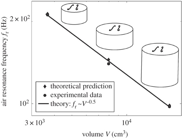
Experimental verification of theoretical f-hole conductance. Theoretical boundary element method predictions (diamonds) and experimental measurements (circles) of air-resonance frequency show excellent agreement (RMSE ≈ 1%). A receiver is placed inside an instrument with rigidly clamped walls. An acoustical source is placed outside the instrument. Expected V −0.5 dependence of the air resonance frequency for a rigid instrument is observed. The conductance of the two interacting violin f-holes is determined from equation (2.3) in theoretical predictions. The air-resonance frequency is taken to be the average of the half-power frequencies measured on either side of the air-resonance peak and is found to have insignificant variation of less than 1% across multiple measurements.
A circular hole is found to provide a poor approximation to a sound hole of the same area but with a significantly different perimeter length, as shown in figure 10, where conductance is found to be linearly proportional to outer perimeter length as explained in §4 and proved in §3. A sound-hole area-based approach, that the conductance of a sound hole is the same as that of a circular hole with same area, then results in incorrect values of Helmholtz resonance frequencies as shown in figure 10 for a variety of sound hole shapes spanning many different musical instruments, based on theory and direct experimental measurements, including the violin f-hole. For example, instruments whose sound holes have interior rosettes, such as lutes, theorbos and ouds, have less sound-hole area than the circle for the same outer perimeter length, which leads to significant errors in the sound-hole area approach. This is consistent with Rayleigh's supposition that for fixed area, the circle is the shape with the lowest conductance [3].
Figure 10.

Conductance-based theory accurately estimates (RMSE ≈ 1%) Helmholtz resonance frequencies for various sound hole shapes. By contrast, resonance frequencies are incorrectly estimated from the circle-of-same-area approach. The conductance of the interacting sound holes of any instrument with multiple sound holes is determined from equation (2.3). The air-resonance frequency is taken to be the average of the half-power frequencies measured on either side of the air-resonance peak and is found to have insignificant variation of less than 1% across multiple measurements.
A circular hole is also quantitatively found to be a poor approximation to the f-hole by elastic instrument analysis and conductance theory. If sound hole area is fixed, then the Helmholtz resonance frequencies of Cremonese violins with circular holes are offset by roughly 50 Hz or three semitones from those of violins with f-holes (electronic supplementary material, figure S1). If sound hole perimeter length is fixed, then the resonance frequencies are offset by roughly 100 Hz or 6 semitones from those of violins with f-holes (electronic supplementary material, figure S1). Cremer [9] deduced that an ellipse of the same area is a better approximation to an f-hole than a circle of the same area but did not quantify the accuracy of this approximation in conductance, radiated power or resonance frequency due to the lack of a method for computing the conductance of an actual f-hole.
8. Experimental verification of differences between rigid and elastic Helmholtz resonance for the violin
By experimentally stimulating a violin with an external sound source and an internal receiver, the measured Helmholtz resonance frequency of a violin with rigidly clamped top and back plates is found to provide an excellent match (figure 11), within roughly 1% after repeated measurements, to the rigid instrument Helmholtz resonance frequency of equation (4.3) with f-hole conductance theory (§§2 and 3). The plates are clamped using five c-clamps attached approximately uniformly across the violin plates. When the plate clamps are removed, air resonance frequency is found to be reduced by roughly 6±1% (figure 11) from the clamped case after repeated measurements, consistent with the reduction expected from elastic volume flux analysis (§9) with f-hole conductance theory (§§2 and 3) (figure 4b). This experimentally shows that the elastic effects of the violin body lead to a roughly 6% reduction in Helmholtz resonance frequency from that of a corresponding rigid violin body.
Figure 11.
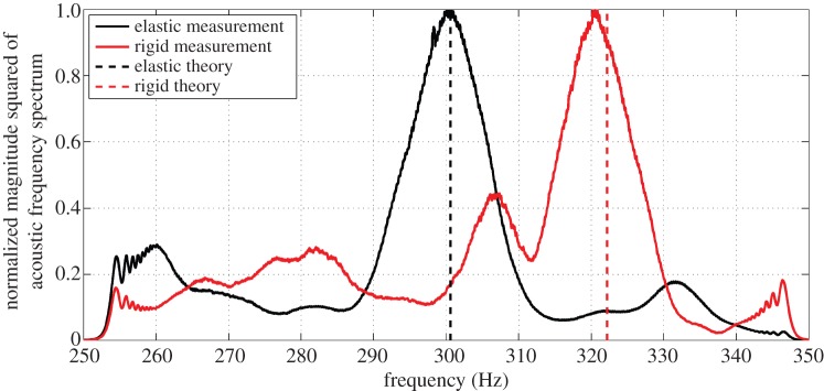
The measured Helmholtz resonance frequency of a violin with rigidly clamped top and back plates (solid red curve) is an excellent match (within roughly 1%) to the rigid instrument analysis (equation (4.3), dashed red line). When the plate clamps are removed, the measured resonance frequency (solid black curve) reduces by roughly 6% or a semitone, consistent with the reduction expected from elastic volume flux analysis for the violin (dashed black line). The two spectra shown are normalized by their respective peak amplitudes. The violin is externally stimulated with white noise. The violin used here has LF=70.5 mm, V =1580 cm3, hsh=2.7 mm, ha=35.9 mm, htop=2.5 mm and hback=3 mm. Other physical parameters are given in table 1.
9. Harmonic oscillation of violin elastic structure coupled with compressible air and f-hole air flow at air resonance
At air resonance measurements have shown that the violin radiates sound as an omni-directional or monopolar source [1], as has also been noted in [53]. Sound radiation at air resonance can then be determined from the total volume flux due to air volume flowing through the f-holes and violin body volume change. For the guitar, the lowest mode of vibration, that at air resonance, has been modelled [21,54] by coupling the elastic deformation of the guitar with fluid compression within the air cavity using a fundamental harmonic oscillator approach. This work followed earlier suggestions of considering a similar harmonic oscillator approach for the violin [20]. It was found that the guitar's elastic body led to a significant lowering of the air cavity resonance frequency from that of a corresponding rigid instrument [55] given by the classical theory of a Helmholtz resonator [3–5]. Here, a similar reduction in air cavity resonance frequency is experimentally found by investigating a rigidly clamped versus a free, unclamped violin and theoretically confirmed as shown in §8. This similarity between guitar and violin results suggests rigid analysis is inadequate and elastic analysis, as was applied to the guitar [21,54], is necessary to estimate the air resonance frequency of a violin to within a semitone.
At and in the vicinity of the air resonance frequency, it has been experimentally shown that roughly normal displacements of the top and back plate of the violin are primarily responsible for radiation of sound [8,13]. This is consistent with measured monopole radiation at the air resonance frequency since monopole radiation results from pure volume change. The spectral peak at the air resonance frequency is a result of harmonic oscillation involving masses, stiffnesses and damping components from the violin. Measurements across extant classical Cremonese violins [43–45] show the air resonance frequency to be remarkably stable, varying within only two-thirds of a semitone (≈4%) with a standard deviation of only one-third of a semitone (≈2%). This suggests that a stable physical mechanism is at work at air resonance. The harmonically oscillating structural elements of the violin that lead to sound radiation at air resonance have stiffnesses that have been identified in previous studies [56] (electronic supplementary material, §6). In particular, at the air resonance frequency, the ribs and sound post correspond to nulls in the displacement field of the violin top and back plates [8,57], and so these regions yield negligible contributions to both volume change and the resulting monopole radiation. The ribs and sound post, however, add stiffness to the violin top and back plates, which affects the displaced volume. The stiffness of an actual violin top plate, , of thickness with sound holes, curvature and structural support from the bass bar, sound post and ribs has been experimentally [56] determined through spectral analysis (electronic supplementary material, §6). The stiffness of an actual violin back plate, , of thickness with curvature and structural support from the sound post and ribs has been experimentally [56] determined through spectral analysis (electronic supplementary material, §6). Elastic coupling of the air cavity, with compressibility , to the violin structure plays an important role at air resonance, as does the combined conductance of the sound holes, C, which regulates volume changes due to air volume flow, vair, through the sound holes. When the system is subjected to top plate forcing F at the bridge, the resulting harmonic oscillation can be described using Newton's second law. The total structural volume change resulting from this oscillation can be determined via multiplication of equivalent displaced areas (electronic supplementary material, §6) Stop and Sback of the top and back plates at air resonance, which include the combined effects of the curved violin shape and nonlinear modal displacement field, with associated time-dependent normal displacements xtop(t) and xback(t) of the top and back plates (electronic supplementary material, §6). The ratios of equivalent displaced area to total plate surface area for actual violin top and back plates at air resonance have been experimentally determined (electronic supplementary material, §6) from holographic measurements [57].
The air-resonance dynamics of i=1,2,3,…N Cremonese violins beginning from Amati 1560 to Guarneri 1745, where N=485 are analysed. Known design parameters Ci (electronic supplementary material, §9), V i, htopi, hbacki and hai from direct measurements or interpolation appear in figures 4c and 5. Small variations in top plate thickness htopi about for the ith violin lead to top plate stiffness near air resonance where ϵtop is the first-order Taylor series coefficient. Similarly, back plate stiffness near air resonance depends on plate thickness hbacki, where ϵback is the first-order Taylor series coefficient for small variations near . The equivalent displaced top plate and back plate areas (electronic supplementary material, §6) that contribute to acoustic radiation via net volume change near air resonance are given by and , where and are the total top and back plate areas. The displaced masses of the top and back plates near air resonance are then and . Damping factors at air resonance
| 9.1 |
are determined such that the energy dissipated by the damping forces acting on the plates and air piston is equal to that acoustically radiated from plate oscillations and air flow through the sound holes (electronic supplementary material, §3), where constants ρtop and ρback are top and back plate densities, respectively. Viscous air flow damping at the sound hole is at least one order of magnitude smaller than radiation damping [10] at air resonance and is negligible. In the guitar model [21,54], damping coefficients were empirically determined by matching modelled and measured sound spectra and/or plate mobility. The physical approach for determining the damping coefficients used here follows Lamb [4], through a radiation damping mechanism. The Q-factors obtained here for the air resonance peaks and the corresponding half power bandwidth are within roughly 20% of those measured for violins [13,58], indicating that radiation damping is the dominant source of damping at the air resonance frequency.
Narrowband [31,59–61] forcing that is spectrally constant in the vicinity of the air resonance peak is assumed, where F0(t) is a slowly varying temporal envelope that is the same for each of the i=1,2,3,…N violins. This allows narrowband approximations [31,59–61] for the displacements , and , where χtopi(t), χbacki(t) and γairi(t) are slowly varying temporal envelopes that are effectively constant at the center of the time window for the ith violin. The harmonic oscillating system at air resonance for the ith violin can then be described by
| 9.2 |
where
| 9.3 |
Estimates of the parameters , , ξtop, ξback, ϵtop and ϵback at the air resonance frequency are obtained by comparing measured air resonance frequency data of Cremonese violins with those obtained from electronic supplementary material, equation (S9) via the method of least squares. Twenty-six air resonance frequency measurements previously obtained in the literature corresponding to 26 extant Cremonese violins [43–45] are used. Parameter ranges in the least-squares estimate are constrained to be near independently measured values. Specifically, the parameters , , ξtop and ξback are all constrained to have small first-order variations, i.e. no more than roughly 33%, from empirical values determined from direct measurements by Jansson and colleagues [56,57] of an actual violin top plate with f-holes, curvature, bass bar and effectively zero displacement at the location of the sound post and ribs (electronic supplementary material, §6) and a violin back plate with curvature, and effectively zero displacement at the location of sound post and ribs (electronic supplementary material, §6). The sum of the squared differences between measured and estimated air resonance frequencies
| 9.4 |
is minimized with respect to parameters , , ξtop, ξback, ϵtop and ϵback resulting in the least-squares estimates
| 9.5 |
where i=1,2,…N and s[i]=1 for the ith violin if air resonance frequency data ωair-datai are available, otherwise s[i]=0. These least-squares estimates are also the maximum-likelihood estimates because the measured air resonance frequencies are uncorrelated and have roughly the same variance across time, and so have minimum variance for large samples [61,62].
Estimates for , , , , and are provided in table 1. These least-squares estimates are used to determine the air resonance frequency ωairi via electronic supplementary material, equation (S9) and xtopi , xbacki and vairi via equation (9.2) in the vicinity of the air resonance peak given the violin design parameters of figures 4c and 5 for the ith violin. The total radiated power at air-resonance is then determined from the resulting xtopi , xbacki and vairi via equation (9.8) for the ith violin. This leads to the time series of air resonance frequency and power shown in figure 4a–b. Empirically obtained dependencies of the air resonance frequency and power on violin design parameters over the entire Cremonese period are given in equations (4.4) and (4.5), respectively. Time series of estimated air-resonance frequency and half power bandwidth about the resonant peak, determined from equation (9.7) (electronic supplementary material, figure S2), characterize the resonance peaks estimated for each violin in the time series [63]. Wood densities are taken to be ρtop=400 kg m−3, ρback=600 kg m−3 [8] and air densities and sound speeds are taken to be cair=340 m s−1 and ρair=1 kg m−3 [64].
Table 1.
Parameters estimated in elastic volume flux analysis.
| parameter | value |
|---|---|
| for | 6.92×10⁴ N m−1 |
| for | 2.75×10⁵ N m−1 |
| for top plate thickness variation near | 1.10×10⁷ N m−2 |
| for back plate thickness variation near | 1.20×10⁸ N m−2 |
| 0.15 | |
| 0.22 |
The second and third eigenvalues, where and of the equation (9.2) system are also estimated from electronic supplementary material, equation S9 for all i=1,2,3…N violins with the parameters of table 1. The RMSE between the means of estimated first eigenvalues and those measured [43–45] from classical Cremonese violins for each family workshop is roughly 1%. Over the entire Cremonese period, the second and third eigenvalue estimates are (i) within roughly 15% of those measured from a modern violin in [56,57], and (ii) consistent with the range found for extant Cremonese violins [7–9,13,20,43,56,57]. Air resonance frequency is found to be relatively insensitive to typical changes in plate stiffness and equivalent displaced areas. For variations in plate stiffnesses of roughly 33% and equivalent displaced areas of roughly 33%, the air resonance frequency varies only by roughly 2%. Mode 1, the air resonance frequency mode, is dominated by resonant air flow through the sound holes, where top and back plates move in opposite directions, and the back plate moves in the same direction as air flow through the sound hole. Mode 2 is mainly influenced by the top plate [13,65]. Mode 3 is mainly influenced by the back plate [13,65]. These basic coupled oscillator results are consistent with the dominant ‘A0,’ ‘T1’ and ‘C3’ motions that Jansson [8] and Moral & Jansson [13] empirically found to contribute significantly to sound radiation near air cavity resonance (figs 2b, 4 and 6 of [13]). Other modes in this frequency range are due to torsional motions that do not lead to significant volume flux nor consequent monopole radiation. Jansson et al. [13] empirically found these torsional modes lead to only insignificant acoustic radiation. Fletcher & Rossing [66] provides a translation of nomenclatures used by various authors for violin modes.
The effect of the ‘island’ area between the sound holes is included in the least-squares stiffness estimates and in those from the empirical measurements of Jansson and colleagues [56,57] as shown in the electronic supplementary material, §6. While dynamical effects associated with the ‘island’ area [9,20,67] between the f-holes have been discussed in the context of violin performance in the 2–3 kHz frequency range, i.e. near the ‘bridge hill’ [68,69], empirical measurements [8] and numerical simulations [67] of violins with and without f-holes, and consequently with and without the ‘island,’ show that the effects of the ‘island’ at air resonance on radiated power and the air resonance frequency are negligible, as shown in the electronic supplementary material, §6. All of these findings are consistent with the fact that at the air resonance frequency only total volume change needs to be accurately resolved. An investigation of the evolution of violin power efficiency at frequencies much higher than the air resonance frequency is beyond the scope of the air resonance analysis presented.
It is theoretically confirmed that at air resonance the combination of elastic displacements of the violin plates and air flow through the sound holes described in equation (9.2) leads to predominantly monopolar radiation in the electronic supplementary material, §4. The spectrum of the radiated acoustic pressure field from a monopole source [2–4] at frequency f is
| 9.6 |
where are Fourier transform pairs and is mass flow rate. The corresponding radiated power spectral density [10] from the monopole at frequency f is
| 9.7 |
where T is the averaging time. The total power in the half power band Δf about the air resonance spectral peak at resonance frequency fair is
| 9.8 |
For the violin, which radiates as a monopole at air resonance (equation (9.6)), the total radiated acoustic power in half-power bandwidth at air resonance is then given by equation (9.8), with and , where , , , and are Fourier transform pairs [31], and vair(t), xtop(t) and xback(t) are estimated from equation (9.2), fair=fair-elastic from equation (4.4) and Δf=Δfair-elastic from equation (9.7). This is consistent with the experimental findings of Meyer [1] and the monopole radiation assumption in a number of musical acoustics applications [21,66,67,70,71]. Well below air resonance, it is theoretically confirmed in electronic supplementary material, §4, that the volume change caused by violin plate displacements is approximately balanced by air flow out of the sound holes leading to approximately dipole radiation
| 9.9 |
where h0 is the distance between the violin centre and top plate, corresponding to the dipole length between volume change sources, and θ is the angle between the receiver and dipole axis along the surface normal pointing outward from the top plate. This is consistent with the experimental findings and discussion of Weinreich [53].
10. Conclusion
By theoretical proof, experimental measurements and numerical computation, air flow at the perimeter rather than the broader sound-hole area is found to dominate the acoustic conductance of sound holes of arbitrary shape, making conductance proportional to perimeter length. As a result, it is found that the ratio of inefficient, acoustically inactive to total sound-hole area was decimated and radiated acoustic power efficiency from air-cavity resonance roughly doubled as sound-hole geometry of the violin's ancestors slowly evolved over nearly a millennium from simple circles of the tenth century to the complex f-hole of the sixteenth–eighteenth centuries. It is also found that f-hole length then followed an increasing trend during the classical Cremonese period (sixteenth–eighteenth centuries) in the renowned workshops of Amati, Stradivari and Guarneri, apparently favouring instruments with correspondingly higher air-resonance power. Temporal power trends due solely to variations in sound hole geometry over roughly a millennium, determined from exact analytic solutions for equivalent rigid violins and infinite rigid sound hole bearing plates, are found to be similar to those determined from elastic volume flux analysis. Resonance frequency and power changes over the classical Cremonese period were then also estimated by elastic volume flux analysis including the variations of other violin parameters as well as f-hole length. This was done by constructing time series of f-hole length, air cavity volume, top and back plate thickness, plate thickness near f-holes and mean air cavity height from measurements of 470 classical Cremonese violins. The resulting temporal trend in radiated power is dominated by the effect of variations in f-hole length alone. This trend is similar to that obtained by exact analytic solutions for equivalent rigid violins and infinite rigid f-hole bearing plates, where only f-hole length is varied. The resulting resonance frequency estimates from elastic analysis match measured resonance frequencies from extant classical Cremonese violins to within a quarter of a semitone, roughly a Pythagorean comma. Rigid analysis, which only depends on f-hole length and cavity volume, leads to the same resonance frequency trend but with an offset of roughly a semitone. This indicates that elastic analysis is necessary for fine-tuned musical pitch estimates. Evolution rate analysis was performed on the time series of measured f-hole length and estimated air resonance power. The corresponding evolution rates are found to be consistent with (a) instrument-to-instrument mutations arising within the range of accidental replication fluctuations from craftsmanship limitations and subsequent selection favouring instruments with higher air-resonance power, rather than (b) drastic preconceived design changes from instrument-to-instrument that went beyond errors expected from craftsmanship limitations. This suggests evolutionary mechanisms by either (i) a conservative approach where planned mutations avoided changes of a magnitude that exceeded those inevitable from normal craftsmanship error, or (ii) purely random mutations from craftsmanship limitations and subsequent selection. The former is consistent with a practical and economical innovation strategy to minimize waste.
Supplementary Material
Acknowledgements
We thank Ryan Fini, Cory Swan and Garret Becker, who helped in Cremonese data reduction and Amit Zoran for help with laser cutting of sound holes. For many interesting and motivating discussions, we thank early instrument and violin makers, professional musicians and museum curators Stephen Barber, Stephen Gottlieb, Sandi Harris, Martin Haycock, Olav Chris Henriksen, Jacob Heringman, Darcy Kuronen, Michael Lowe, Ivo Magherini, Benjamin Narvey, Andrew Rutherford, Lynda Sayce and Samuel Zygmuntowicz.
Data accessibility
All data sources are provided in the electronic supplementary material.
Author contributions
Work on evolution rates, evolution rate thresholds and mutation analysis was primarily done by A.D.J. and N.C.M.; work on elastic and rigid vessel modeling was primarily done by Y.L., A.D.J. and N.C.M.; conductance analysis was primarily done by Y.L., H.T.N., A.D.J. and N.C.M.; acquisition and reduction of Cremonese violin data was primarily done by A.D.J. and R.B.; work on conductance experiments was primarily done by H.T.N., M.R.A., Y.L. and N.C.M.; violin air cavity volume modeling was primarily done by H.T.N., R.B. and N.C.M.; acoustic radiation theory was primarily derived by A.D.J., Y.L. and N.C.M.; Y.L. co-supervised the overall project; N.C.M. conceived and supervised the overall project and N.C.M., A.D.J. and Y.L. wrote the paper. All authors gave final approval for publication.
Funding statement
This research was partially supported by Massachusetts Institute of Technology, North Bennet Street School and the Office of Naval Research.
Conflict of interests
We have no competing interests.
References
- 1.Meyer J. 1972. Directivity of the bowed stringed instruments and its effect on orchestral sound in concert halls. J. Acoust. Soc. Am. 51, 1994–2009 (doi:10.1121/1.1913060) [Google Scholar]
- 2.Lighthill J. 1978. Waves in fluids. Cambridge, UK: Cambridge University Press. [Google Scholar]
- 3.Rayleigh BJWS. 1896. The theory of sound, vol. 2 London, UK: Macmillan and Co. [Google Scholar]
- 4.Lamb H. 1925. The dynamical theory of sound. New York, NY: Dover Publications Inc. [Google Scholar]
- 5.Helmholtz H. 1877. On the sensations of tone. [Trans. AJ Ellis] New York, NY: Dover. [Google Scholar]
- 6.Hutchins CM. 1983. A history of violin research. J. Acoust. Soc. Am. 73, 1421 (doi:10.1121/1.389430) [Google Scholar]
- 7.Dunnwald H. 1990. Ein erweitertes Verfahren zur objektiven Bestimmung der Klangqualitat von Violinen. Acta Acust. United Ac. 71, 269–276. [Google Scholar]
- 8.Jansson EV. 2002. Acoustics for violin and guitar makers in the function of the violin. Stockholm, Sweden: Kungl Tekniska Hogskolan, Department of Speech, Music and Hearing. [Google Scholar]
- 9.Cremer L, Allen JS. 1984. The physics of the violin. Cambridge, UK: The MIT Press. [Google Scholar]
- 10.Morse PM, Ingard K. 1968. Theoretical acoustics. New York, NY: McGraw-Hill Book Co., Inc. [Google Scholar]
- 11.Cato DH. 1991. Sound generation in the vicinity of the sea surface: source mechanisms and the coupling to the received sound field. J. Acoust. Soc. Am. 89, 1076–1095 (doi:10.1121/1.400527) [Google Scholar]
- 12.Cremer L, Heckl M, Petersson BAT. 2005. Structure-borne sound: structure vibrations and sound radiation at audio frequencies. Berlin, Germany: Springer. [Google Scholar]
- 13.Moral JA, Jansson EV. 1982. Eigenmodes, input admittance and the function of the violin. Acustica 50, 329–337. [Google Scholar]
- 14.Randel DM. 2003. Harvard dictionary of music. Cambridge, MA: Harvard University Press. [Google Scholar]
- 15.Panton RL, Miller JM. 1975. Resonant frequencies of cylindrical Helmholtz resonators. J. Acoust. Soc. Am. 57, 1533–1535 (doi:10.1121/1.380596) [Google Scholar]
- 16.Bigg GR. 1980. The three dimensional cavity resonator. J Sound Vib 85, 85–103 (doi:10.1016/0022-460X(82)90472-2) [Google Scholar]
- 17.Deskins WG, Winter DC, Sheng H, Garza C. 1985. Use of a resonating cavity to measure body volume. J. Acoust. Soc. Am. 77, 756–758 (doi:10.1121/1.392346) [DOI] [PubMed] [Google Scholar]
- 18.Webster ES, Davies CE. 2010. The use of Helmholtz resonance for measuring the volume of liquids and solids. Sensors 10, 10 663–10 672 (doi:10.3390/s101210663) [DOI] [PMC free article] [PubMed] [Google Scholar]
- 19.Bissinger G. 1998. A0 and A1 coupling, arching, rib height, and f-hole geometry dependence in the 2 degree-of-freedom network model of violin cavity modes. J. Acoust. Soc. Am. 104, 3608–3615 (doi:10.1121/1.423943) [Google Scholar]
- 20.Beldie JP. 1975. Representation of the violin body as a vibration system with four degrees of freedom in the low frequency range. Technical University of Berlin, Berlin, Germany.
- 21.Christensen O. 1982. Quantitative models for low frequency guitar function. J. Guitar Acoust. 6, 10–25. [Google Scholar]
- 22.Saunders FA. 1953. Recent work on violins. J. Acoust. Soc. Am. 25, 491–498 (doi:10.1121/1.1907069) [Google Scholar]
- 23.Vandegrift G, Wall E. 1997. The spatial inhomogeneity of pressure inside a violin at main air resonance. J. Acoust. Soc. Am. 102, 622–627 (doi:10.1121/1.419736) [Google Scholar]
- 24.Bissinger G. 2003. Wall compliance and violin cavity modes. J. Acoust. Soc. Am. 113, 1718–1723 (doi:10.1121/1.1538199) [DOI] [PubMed] [Google Scholar]
- 25.Rossing TD. 2010. Science of string instruments. New York, NY: Springer. [Google Scholar]
- 26.Collins MD. 1992. A self-starter for the parabolic equation method. J. Acoust. Soc. Am. 92, 2069–2074 (doi:10.1121/1.405258) [Google Scholar]
- 27.Yan H, Liu Y. 2011. An efficient high-order boundary element method for nonlinear wave–wave and wave–body interactions. J. Comput. Phys. 230, 402–424 (doi:10.1016/j.jcp.2010.09.029) [Google Scholar]
- 28.Bronshtein IN, Semendyayev KA, Musiol G, Muhlig H. 2007. Handbook of mathematics. Heidelberg, Germany: Springer. [Google Scholar]
- 29.Lamb H. 1895. Hydrodynamics. London, UK: Cambridge University Press. [Google Scholar]
- 30.Comprehensive information about unique Italian stringed instruments. See http://www.cozio.com (accessed 17 April 2013).
- 31.Seibert WM. 1986. Circuits, signals and systems, vol. 2 Cambridge, MA: The MIT Press. [Google Scholar]
- 32.Harwood I, Prynne M. 1975. A brief history of the lute. Richmond, UK: Lute Society. [Google Scholar]
- 33.Sandys W, Forster SA. 1884. History of the violin. Mineola, NY: Dover Publications Inc. [Google Scholar]
- 34.Engel C, Hipkins AJ. 1883. Researches into the early history of the violin family. London, UK: Novello, Ewer & Co. [Google Scholar]
- 35.Van der Straeten ESJ. 1933. The history of the violin: its ancestors and collateral instruments from earliest times to the present day. Cassell and company Ltd. [Google Scholar]
- 36.Baines A. 1992. The oxford companion to musical instruments. New York, NY: Oxford University Press. [Google Scholar]
- 37.Woodfield I. 1988. The early history of the viol. New York, NY: Cambridge University Press. [Google Scholar]
- 38.Hill WH, Hill AF, Hill AE. 1980. Antonio Stradivari, his life and work: 1644–1737. London, UK: W. E. Hill and Sons. [Google Scholar]
- 39.Hill WH, Hill AF, Hill AE. 1980. The violin makers of the Guarneri family, 1626–1762. London, UK: W. E. Hill and Sons. [Google Scholar]
- 40.Prynne M. 1949. An Unrecorded Lute by Hans Frei. Galpin Soc. J. 2, 47–51 (doi:10.2307/841395) [Google Scholar]
- 41.Wells RH. 1981. Number symbolism in the renaissance lute rose. Early Music 9, 32–42 (doi:10.1093/earlyj/9.1.32) [Google Scholar]
- 42.Hubbard R, Schott H. 2002. The historical harpsichord: a monograph series in honor of Frank Hubbard, vol. 4 Hillside, NY: Pendragon Press. [Google Scholar]
- 43.Bissinger G. 2008. Structural acoustics of good and bad violins. J. Acoust. Soc. Am. 124, 1764–1773 (doi:10.1121/1.2956478) [DOI] [PubMed] [Google Scholar]
- 44.Curtin J. 2009. Scent of a violin. The Strad, pp. 30–33.
- 45.Curtin J. 2009. Good vibrations. The Strad, pp. 44–47.
- 46.Price GR. 1970. Selection and covariance. Nature 227, 520–521 (doi:10.1038/227520a0) [DOI] [PubMed] [Google Scholar]
- 47.Fisher RA. 1999. The genetical theory of natural selection: a complete variorum edition. New York, NY: Oxford University Press. [Google Scholar]
- 48.Chiesa C, Rosengard D. 1998. The stradivari legacy. London, UK: P. Biddulph. [Google Scholar]
- 49.Savart F. 1819. Rapport sur un memoire de M. Felix Savart relatif a la construction des instruments a cordes et a archet. Ann. Chim. Phys. 12, 225–255. [Google Scholar]
- 50.Dubourg G. 1852. The violin: some account of that leading instrument, and its most eminent professors, from its earliest date to the present time. London, UK: Robert Cocks and Co. [Google Scholar]
- 51.Larson AP. 2003. Beethoven and Berlioz, Paris and Vienna: musical treasures from the age of revolution & romance, 1789–1848 National Music Museum. ND: Vermillion Press. [Google Scholar]
- 52.Nia HT. 2010. Acoustic function of sound hole design in musical instruments. Master's Thesis, Massachusetts Institute of Technology, Cambridge, MA, USA.
- 53.Weinreich G. 1985. Sound hole sum rule and the dipole moment of the violin. J. Acoust. Soc. Am. 77, 710–718 (doi:10.1121/1.392339) [Google Scholar]
- 54.Christensen O, Vistisen BB. 1980. Simple model for low-frequency guitar function. J. Acoust. Soc. Am. 68, 758–766 (doi:10.1121/1.384814) [Google Scholar]
- 55.Meyer J. 1974. Die Abstimmung der Grundresonanzen von Gitarren. Das Musikinstrument 23, 179–186. [Google Scholar]
- 56.Jansson E, Molin N-E, Sundin H. 1970. Resonances of a violin body studied by hologram interferometry and acoustical methods. Physica Scripta 2, 243–256 (doi:10.1088/0031-8949/2/6/002) [Google Scholar]
- 57.Saldner HO, Molin N-E, Jansson EV. 1996. Vibration modes of the violin forced via the bridge and action of the soundpost. J. Acoust. Soc. Am. 100, 1168–1177 (doi:10.1121/1.416301) [Google Scholar]
- 58.Woodhouse J, Langley RS. 2012. Interpreting the input admittance of violins and guitars. Acta Acust. United Ac. 98, 611–628 (doi:10.3813/AAA.918542) [Google Scholar]
- 59.DiFranco J, Rubin B. 2004. Radar detection. New York, NY: SciTech Publishing Inc. [Google Scholar]
- 60.Levanon N. 1988. Radar principles. New York, NY: Wiley-Interscience. [Google Scholar]
- 61.Kay S. 1998. Fundamentals of statistical signal processing, vol. I–II MA: Pearson Education Inc. [Google Scholar]
- 62.Rao CR. 1965. Linear statistical inference and its applications. MA: John Wiley & Sons. [Google Scholar]
- 63.French AP. 1971. Vibration and waves. Boca Raton, FL: CRC Press. [Google Scholar]
- 64.Everest FA, Pohlmann KC, Books T. 2001. The master handbook of acoustics. New York, NY: McGraw-Hill. [Google Scholar]
- 65.Jansson EV, Niewczyk BK, Fryden L. 1995. On the body resonance C3 and its relation to the violin construction. STL-QPSR 36, 1–10. [Google Scholar]
- 66.Fletcher NH, Rossing TD. 1998. The physics of musical instruments. New York, NY: Springer. [Google Scholar]
- 67.Gough CE. 2013. Vibrational modes of the violin family. In Proc. SMAC2013, pp. 66–74, Stockholm, Sweden.
- 68.Durup E, Jansson EV. 2005. The quest of the violin Bridge-Hill. Acta Acust. United Ac. 91, 206–213. [Google Scholar]
- 69.Woodhouse J. 2005. On the ‘bridge hill’ of the violin. Acta. Acust. United Ac. 91, 155–165. [Google Scholar]
- 70.Weinreich G, Arnold EB. 1980. Method for measuring acoustic radiation fields. J. Acoust. Soc. Am. 68, 404–411 (doi:10.1121/1.384751) [Google Scholar]
- 71.Gough CE. 2013. Acoustic characterization of violin family signature modes by internal cavity measurements. In Proc. SMAC2013, pp. 75–81, Stockholm, Sweden.
Associated Data
This section collects any data citations, data availability statements, or supplementary materials included in this article.
Supplementary Materials
Data Availability Statement
All data sources are provided in the electronic supplementary material.