

Abstract
Local binary pattern (LBP) is a simple gray scale descriptor to characterize the local distribution of the grey levels in an image. Multi-resolution LBP and/or combinations of the LBPs have shown to be effective in texture image analysis. However, it is unclear what resolutions or combinations to choose for texture analysis. Examining all the possible cases is impractical and intractable due to the exponential growth in a feature space. This limits the accuracy and time- and space-efficiency of LBP. Here, we propose a data mining approach for LBP, which efficiently explores a high-dimensional feature space and finds a relatively smaller number of discriminative features. The features can be any combinations of LBPs. These may not be achievable with conventional approaches. Hence, our approach not only fully utilizes the capability of LBP but also maintains the low computational complexity. We incorporated three different descriptors (LBP, local contrast measure, and local directional derivative measure) with three spatial resolutions and evaluated our approach using two comprehensive texture databases. The results demonstrated the effectiveness and robustness of our approach to different experimental designs and texture images.
Keywords: local binary pattern, frequent pattern mining, texture image, feature selection, classification
1. INTRODUCTION
Texture analysis has a wide variety of applications in image processing and computer vision such as image segmentation (Malik, Belongie, Leung, & Shi, 2001), image retrieval (Howarth & Rüger, 2005) (Manjunath & Ma, 1996), object recognition (Samal, Brandle, & Zhang, 2006) (Tan & Triggs, 2007), medical image analysis (Castellano, Bonilha, Li, & Cendes, 2004) {Kwak, 2014 #95}, and remote sensing (C. Zhu & Yang, 1998). Numerous methods are available to extract robust and reliable texture information from an image. These include a co-occurrence matrix (Haralick, Shanmugam, & Dinstein, 1973), Markov Random Field (MRF) (Cross & Jain, 1983), Gabor filtering (Bovik, Clark, & Geisler, 1990), wavelet transform (Laine & Fan, 1993), principal component analysis (PCA) (Turk & Pentland, 1991), and local discriminative analysis (LDA) (Etemad & Chellappa, 1997). Recently, a local texture descriptor, called local binary pattern (LBP) (Ojala, Pietikainen, & Maenpaa, 2002), has gained much attention due to its low computational complexity, gray-scale and rotation invariance, robustness to illumination changes, and excellent performance in many applications (Ahonen, Hadid, & Pietikainen, 2006) (Wang, Gong, Zhang, Li, & Zhuang, 2006) (Nanni, Lumini, & Brahnam, 2010) (Tajeripour, Kabir, & Sheikhi, 2008) (G. Zhao & Pietikainen, 2006).
LBP is a simple descriptor that compares the gray level of a pixel and its local neighborhood and generates a binary pattern code. Binary pattern codes are often summarized into a histogram, and a bin in the histogram corresponds to a unique binary code. Numerous variants of LBP have been proposed to improve upon the basic LBP. It includes variants in neighborhood topology (Shu Liao & Chung, 2007) (Wolf, Hassner, & Taigman, 2008) (Petpon & Srisuk, 2009) and thresholding and/or encoding (Jin, Liu, Lu, & Tong, 2004) (Tan & Triggs, 2007) (Fu & Wei, 2008) (Iakovidis, Keramidas, & Maroulis, 2008) (Z. Guo, Zhang, & Zhang, 2010) (Nanni, et al., 2010) (Zhenhua Guo, Zhang, Zhang, & Zhang, 2010) (B. Zhang, Gao, Zhao, & Liu, 2010) (Zhenhua Guo, Li, You, Zhang, & Liu, 2012) (C. R. Zhu & Wang, 2012). Some researchers have also proposed alternative manners of exploiting the binary pattern codes; for example, “uniform” patterns group the binary pattern codes by the number of bit transitions. Linear or non-linear dimensionality reduction methods sought to utilize only the useful pattern codes (Topi, Timo, Matti, & Maricor, 2000) (S. Shan, Zhang, Su, Chen, & Gao, 2006) (Chan, Kittler, & Messer, 2007) (D. Zhao, Lin, & Tang, 2007) (Hussain & Triggs, 2010) (Smith & Windeatt, 2010) (C. Shan, Gong, & McOwan, 2005) (Lumini, 2010) (Nanni, Lumini, & Brahnam, 2012).
Although LBP and its variants perform well, their combinations often outperform the individual descriptors; for instance, a multi-resolution LBP showed an improvement over single resolutions (Ojala, Pietikainen, et al., 2002) (Zhenhua Guo, et al., 2012) and a joint histogram of LBP and a variance measure descriptor of local contrast (VAR) outperformed each of the descriptors (Ojala, Pietikainen, et al., 2002). Combining complementary descriptors in a multi-resolution setting appears to be best utilizing the capability of LBP. However, a simple approach of integrating several LBP variants into a single- or multidimensional histogram may be undesirable. There are many LBP variants and numerous ways to combine them. Each combination is represented in a high-dimensional feature space. Estimating the exact densities or probabilities of such features requires huge training images, and noisy features would adversely affect texture analysis (Ojala, Pietikainen, et al., 2002). Conventional dimensionality reduction methods may be ineffective because it is still restricted to how the initial feature pool was prepared and may lead to another issue of interpreting the resulting (or transformed) features or an additional computational burden on a testing phase. Hence, an alternative, efficient, and effective method to fully utilize LBP and its variants is needed.
In this paper, we propose a data mining approach for LBP and its variants (Figure 1). The basic and variants of LBP with multiple radii are computed, and frequent pattern mining discovers the binary pattern codes that frequently occurred within training images. The frequently occurred pattern codes can be any combination of LBP and its variants and form the initial feature pool. Since they are frequent, the density (or probability) estimation is reliable. A two-stage feature selection method selects the most discriminative features. In the first stage, features are ordered by their relevance with the given class labels using a mutual information-based criterion. In the second stage, forward feature selection chooses the best feature set with the highest discriminative capability on the training images. A histogram is built using the selected features and used for texture analysis. We evaluate our approach on the texture images from the public texture databases.
Figure 1.

Illustration of our proposed framework. Pattern codes are individually generated using LBP, VAR and LDDP with 8 neighbors and a radius 1 for the given images. Frequent patterns are mined with a minimum support threshold (MINSUP) θ and mutual information-based feature selection method chooses the most discriminative patterns. Finally, classification models (or histograms) are constructed for the images.
The rest of the paper is organized as follows. In Section2, we briefly review LBP and its variants. In Section 3, we describe our approach. In Section 4, training and validation datasets are presented. In Section 5, the experimental results are demonstrated. Finally, we conclude in Section 6.
2. LOCAL BINARY PATTERN AND ITS VARIANTS
2.1. Basic LBP
Local binary pattern (LBP) (Ojala, Pietikainen, et al., 2002) is a gray scale texture descriptor that utilizes the distribution of the gray levels of local neighborhood pixels. Given a (center) pixel c in an image I (Figure 2), it examines its neighboring pixels p(p = 0, …, P − 1) in a radius R and generates a binary pattern code as follows:
| (1) |
| (2) |
where gc and gp represent the gray level of the center pixel and its neighborhood pixels, respectively. The coordinates of the neighborhood pixels are computed as (R cos(2πp/P), −R sin(2πp/P)) and their gray levels are estimated by interpolation. Since LBP only depends on the sign of the gray level difference, the pattern code is invariant to the scaling of the gray scale. Moreover, rotating the image, the gray level of the neighborhood pixels rotates around the center pixel. The rotation results in a different binary pattern code but only makes a bit-wise shift in the original pattern code. Hence, rotation-invariant pattern code is computed as
Figure 2.

Description of LBP computation. A binary code is computed for a pixel c (red circle) and its 8 neighborhood pixels in a radius 1 and further converted to a decimal number. A black and white circle denote a binary digit of 0 and 1, respectively, generated by a thresholding function s(·). gc and gp correspond to the gray level of the center pixel c and the neighborhood pixels p(p = 0, …, P − 1), respectively. LBPP,R denotes LBP using P neighborhood pixels in a radius R. and represent rotation-invariant and “uniform” rotation-invariant LBPs, respectively.
| (3) |
where ROR(x, i) is a circular bit-wise shift operator on x by i bits. Limiting the number of bit transitions (from 0 to 1, or vice versa), “uniform” pattern is defined as follows:
| (4) |
| (5) |
It is known that “uniform” patterns discard a large amount of the binary pattern codes that could provide useful and discriminative information in an image (Zhou, Wang, & Wang, 2008). In addition, LBP lacks contrast information. To compensate for it, variance of the local contrast (VAR) is measured as follows:
| (6) |
Computing LBP, a histogram is often built over a whole image or a region of an image and used for texture analysis. When multiple LBPs from different radii or LBP variants are computed, either a joint histogram is constructed or histograms are concatenated into one large histogram.
2.2. Thresholding and Encoding
Some variants incorporate different thresholding or binary code encoding schemes. Improved LBP (ILBP) (Jin, et al., 2004) calculates the mean gray level in a local neighborhood and uses it as a threshold. It assigns the largest weight to the center pixel which contains more information than the neighborhood pixels. Centralized binary pattern (CBP) (Fu & Wei, 2008) compares pairs of neighboring pixels and decreases the length of a histogram. In Completed LBP (CLBP) (Z. Guo, et al., 2010), three different types of information (sign difference, magnitude difference, and intensity) is computed and combined into one large histogram. Weighted Local Gray Level (WLG) is further introduced to CLBP (Y. Zhao, Jia, Hu, & Min, 2013). Local Ternary Patterns (LTP) (Tan & Triggs, 2007) extends LBP by introducing 3-valued codes (1, 0, and −1). For computational simplicity, the ternary code is further split into two LBPs using positive and negative parts only. Two separate histograms are built for each LBP and then combined into a single histogram. Completed LTP (CLTP) extends LTP by decomposing the local difference into two sign complementary components and two magnitude complementary components (Rassem & Khoo, 2014).
Elongated Quinary Pattern (EQP) (Nanni, et al., 2010) utilizes a quinary encoding and elliptical neighborhood topology. Similar to LTP, four histograms are constructed and concatenated into one large histogram. Instead of the hard thresholding of LBP, Fuzzy LBP (FLBP) (Iakovidis, et al., 2008) introducs fuzzy logic to LBP with the following rules: 1) The more negative Δgp is, the greater the certainty that s(Δgp) is 0 2) The more positive Δgp is, the greater the certainty that s(Δgp) is 1 where Δgp = gp − gc. Based upon the two rules, two membership functions are defined and used to construct the FLBP histogram. Adaptive LBP (ALBP) (Zhenhua Guo, Lei Zhang, David Zhang, & Su Zhang, 2010) incorporates orientation information into LBP by minimizing the directional difference along different orientations. Local Derivative Pattern (LDP) (B. Zhang, et al., 2010) attempts to encode higher order derivative information which provides more detailed texture information. However, it is four times longer than LBP and its framework differs from LBP. A simpler and more efficient method is proposed by Local directional derivative pattern (LDDP) (Zhenhua Guo, et al., 2012). LDDP computes the 2nd, 3rd, and 4th order derivatives along p direction as follows:
| (7) |
| (8) |
| (9) |
where , and denote the gray level of a neighborhood pixel p in a circle of radius R1, R2, and R3, respectively. The mth order LDDP is computed as follows:
| (10) |
Local Binary Count (CLBC) only utilizes the number of 1s in a neighborhood (Y. Zhao, Huang, & Jia, 2012). In (Ghahramani, Zhao, & Pietikainen, 2013), intensity information is incorporated into LBP. In Robust LBP (RLBP), noisy coding bits are identified and revised to improve LBP (Chen, Kellokumpu, Zhao, & Pietikainen, 2013). Local structure is also incorporated into LBP (Shrivastava & Tyagi, 2014). Dominant Neighborhood Structure (DNS) is combined with LBP (Khellah, 2011). Neighborhood estimated local binary patterns (NELBP) are proposed (Song & Yan, 2014).
2.3. Neighborhood topology
Local Line Binary Pattern (LLBP) (Petpon & Srisuk, 2009) considers neighborhood pixels in a straight line. The gray level of a center pixel is separately compared to its neighboring pixels in a horizontal and vertical direction. Then, the magnitude of LLBP is computed as the square root of the sum of the squared horizontal and vertical responses. Elongated LBP (ELBP) (Shu Liao & Chung, 2007) adopts an elliptical neighborhood topology including three parameters: 1) major axis A 2) minor axis B 3) number of neighborhood pixels P. Patch-based LBP draws a w × w patch around a center pixel and its neighborhood pixels and compares the values of the patches to generate a binary code. Three-Patch LBP (TPLBP) (Wolf, et al., 2008) compares a center patch and two neighborhood patches which are ∝ apart from each other in a circle and produces a single bit depending on which of the two patches is closer to the center patch. Four-Path LBP (FPLBP) (Wolf, et al., 2008) uses two circles. A pair of center symmetric patches in an inner circle is compared with those in an outer circle. Multi-ring local binary pattern (MrLBP) (Y. G. He & Sang, 2013) creates pattern codes from several ringed areas.
2.4. Multi-scale Analysis
Block- or region- based multi-scale analyses have been proposed for LBP. In Multi-scale Block Local Binary Pattern (MB-LBP) (Shengcai Liao, Zhu, Lei, Zhang, & Li, 2007), a neighborhood pixel is replaced by a small block, and the mean gray level of the small block is used to generate a binary pattern code. (Mäenpää & Pietikäinen, 2003) adopts a Gaussian low-pass filter. It extracts texture information from a larger area than a single pixel while minimizing redundant information. Then, cellular automata are applied for encoding arbitrarily large neighborhoods and generating eight bits automata rules. Another multi-scale analysis scheme is to utilize image pyramids at different scales. In (Turtinen & Pietikäinen, 2006), LBPs at three different image scales are extracted and concatenated for texture image classification. It divides an image into non-overlapping blocks. Windows of three different sizes are placed at the center of each block, and the blocks at different scales are scaled to the same size prior to computing LBP. Similarly, (Y. He, Sang, & Gao, 2011) generates image pyramids by applying five different templates including a Gaussian kernel and four anisotropic filters. LBPs are computed from the original image and the image pyramids to describe macro and micro structures of texture images. In addition, Hierarchical multi-scale LBP (Zhenhua Guo, Zhang, Zhang, & Mou, 2010) utilizes “non-uniform” pattern codes. First, it computes LBP from the largest radius and groups the pixels into “uniform” and “non-uniform” pattern groups. Second, a histogram is built for the “uniform” patterns. Third, for those “non-uniform” patterns, LBP is computed with a smaller radius. Repeating the above three steps until it reaches the smallest radius, all the histograms with different radii are, finally, combined into one multi-scale histogram. In MBLTP (Xiaofei, et al., 2013), LTP is computed based on the average value of blocks. Polytypic multi-block LBP (P-MLBP) (Li, Ruan, Jin, An, & Zhao, 2015) fuses depth and texture information to represent three-dimensional facial expressions.
2.5. Discriminative Pattern and Feature Selection
“Uniform” pattern reduces the number of patterns by merging a large number of “non-uniform” patterns into one group. (Yang & Wang, 2007) and (Zhou, et al., 2008) further assigns part of “non-uniform” patterns to “uniform” patterns. (Yang & Wang, 2007) adopts Hamming distance between patterns. (Zhou, et al., 2008) utilizes the occurrence of bits and structure of 1s and 0s in a binary code. Dominant LBP (DLBP) (S. Liao, et al., 2009) considers only the most frequently occurred patterns. It determines the number of dominant patterns: 1) Sort patterns by their frequencies in non-decreasing order 2) Find the number of patterns comprising 80% of the entire pattern occurrences. (Y. Guo, Zhao, Pietikäinen, & Xu, 2011) uses fisher separation criterion (FSC) to provide the most reliable and robust DLBP. By combining DLBPs of different classes, they formed a global DLBP.
Search-based methods have been proposed. (Topi, et al., 2000) finds the optimal subset of patterns using beam search. Starting from a single pattern, it iteratively increases the size of the pattern set and retains the best pattern set so far. The goodness of the pattern set is determined by a classification error. Fast correlation-based filtering (FCBF) (Smith & Windeatt, 2010) takes a similar approach but introduces information-theoretic concept of symmetric uncertainty to measure a correlation between patterns and class labels. It repeatedly selects the most correlated pattern with the given class labels and rejects patterns that are more correlated with the selected pattern than the class labels. Moreover, boosting has been another popular feature selection method. (G. Zhang, et al., 2005) generates sub-images with scalable sub-windows and extracts LBPs from each of the sub-images. Applying AdaBoost, the most discriminative sub-images are selected. Also, (C. Shan & Gritti, 2008) uses AdaBoost to select the most discriminative LBP histogram bins.
Another dimensionality reduction approach is to transform or project a high-dimensional LBP feature space into a lower dimensional space. (Chan, et al., 2007) uses Linear Discriminant Analysis (LDA) in conjunction with principal component analysis (PCA) to derive discriminative patterns from a high-dimensional multispectral LBP. Using Laplacian PCA (LPCA), (D. Zhao, et al., 2007) attempts to maximize the weighted local scatter instead of the global scatter of data as in the original PCA. (S. Shan, et al., 2006) uses Ensemble of Piecewise Fisher Discriminant Anlalysis (EPFDA) classifiers with LBP and local Gabor binary pattern (LGBP). LGBP is a simple extension of LBP which applies Gabor transform prior to computing LBP. EPFDA splits the original high-dimensional histogram into k segments. Lower dimensional features are extracted for each of the segments by applying FDA. The final classifier is built by combining all the FDA models together. Partial Least Squares (PLS) dimensionality reduction is employed by (Hussain & Triggs, 2010) to select the most discriminative patterns from the combined set of three different features: LBP, histogram of gradients (HOG), and LTP. (C. Shan, et al., 2005) performs Locality Preserving Projections (LPP) on LBP. In (Lumini, 2010) (Nanni, et al., 2012), PCA and neighborhood preserving embedding (NPE) are applied for random subsets of LBP. They randomly select 50% of the entire LBPs, apply PCA and NPE sequentially, and build a support vector machine (SVM) on the subset. Repeating this procedure 50 times and combining the results, they obtain the final classifier. In (Girish, Shrinivasa Naika, & Das, 2014), PCA is combined with MB-LBP for face recognition.
3. PROPOSED APPROACH
Suppose that we compute K variants of LBP with a radius R for a set of texture images. Each descriptor includes Nk binary codes where is ith binary code of the kth descriptor. Each pixel in an image contains K binary codes , 1 ≤ i1 ≤ N1, 1 ≤ i2 ≤ N2, …, 1 ≤ iK ≤ NK. A unique combination of the binary codes becomes a bin in a joint histogram of the K descriptors. However, computing the joint histogram is not time- and space- effective due to the exponential growth of the number of bins. Even, lots of noisy bins will present. Instead, we attempt to directly find the most informative bins that are frequent and discriminative, i.e. improve discriminative power as well as reduce noisy bins.
In order to find frequent pattern codes (or bins), we adopt a data mining approach, so called frequent pattern mining (Han, Cheng, Xin, & Yan, 2007). Whether a bin is frequent or not is determined by a user-specified threshold. It should be noted that frequent pattern mining discovers any combination of the binary pattern codes that are frequent. This means that we can simultaneously examine not only an individual descriptor but also any combination of the descriptors. It is equivalent to computing and exploring histograms of a single descriptor and joint histograms of every combination of the K descriptors. Hence, “frequent bins” include bins from single- and multiple- descriptor histograms. Since the frequency of a bin is not indicative of its discriminative ability, a two-stage feature selection is followed to obtain a set of discriminative bins (or features). In the first stage, we order the features via mRMR (minimum Redundacy Maximum Relevance) criterion which maximizes the relevance between the features and the class labels and minimizes the redundancy among the features. In the second stage, forward feature selection chooses the most discriminative features according to the mRMR feature order. Finally, classification models are constructed using the discriminative features and tested on the validation datasets.
3.1. FREQUENT PATTERN MINING
Suppose a dataset D = {d1, d2, …, dn} has NA categorical attributes, and class label Y = {y1, y2, …, yn} has NC classes where yi is the label associated with data di. Each attribute can have a number of values, and each pair of an attribute A and a value v (A, v) is mapped to a distinct item in I = {a1, a2, …, am}. Then, each data di is represented as a set of items in I. In the dataset, frequent patterns are the itemsets which occur no less than a user-specified threshold. In other words, an k-itemset α, consists of k items from I, is frequent if α occurs no less than θ|D| times in a dataset, where θ is a user-specified minimum support threshold (MINSUP) and |D| is the total number of data. The support of a pattern is the number of data contains the pattern. We set MINSUP=0.2%. FP-growth (Han, Pei, & Yin, 2000), which generates the complete set of frequent patterns without candidate generation, is used to mine frequent patterns. When we have continuous data, each dimension is independently discretized prior to applying frequent pattern mining. We adopt equal-depth binning which allocates approximately same number of data in each interval.
3.2. Feature Selection
mRMR (Peng, Long, & Ding, 2005) is a feature selection method based on mutual information. It attempts not only to maximize the relevance between selected features and class labels, but also to minimize the redundancy between selected features. Both the relevance and redundancy are characterized in terms of mutual information as follows:
| (11) |
| (12) |
where I(x; y) represent the mutual information of two variables x and y, S is a feature set, and Y is a class label. To achieve the goal of optimizing above two conditions simultaneously, the simple mRMR criterion, max(D − R), is invoked. mRMR starts from a feature with the highest maximal relevance and selects a new feature among the rest of features that is the most correlated with the class labels while being the least redundant with the selected features so far. Thus, it generates an order of the features according to the mRMR criterion. Following the order by mRMR, forward feature selection sequentially adds a new feature at a time and measures the discriminative power of the features so far. The features with the highest classification performance are chosen as the most discriminative features. Performing K-fold cross validation, the classification performance is measured by the ratio of the number of correctly predicted images and the total number of images. K-fold cross validation divides the training dataset into K disjoint partitions, learns classification models on the K−1 partitions, and tests the models on the remaining partition. This is repeated K times with different choices of the testing partition. We set K=5.
3.3. Classification
Histograms (or classification models) are built using the selected features and training images. Validation images are also converted into histograms using the same features. In order to assign a class label for a testing image, we adopt a k-nearest neighbor approach, i.e., the class label of a testing image is determined by its neighbors among the training images. As a measure of similarity between two images (or histograms), we use the following two distance metrics.
| (13) |
| (14) |
where , B is the number of bins, and Tk and Mk are the densities at the kth bin of the testing and model image, respectively.
4. DATASETS
4.1. Outex database
We employed two datasets from Outex database (Ojala, Maenpaa, et al., 2002) (Figure 3a): Outex_TC_00010 (TC10) and Outex_TC_00012 (TC12). Both TC10 and TC12 include the same 24 classes of texture images. Each image was acquired under three different illumination settings (“inca”, “horizon”, and “t184”) and rotated at 9 different angles (0°, 5°, 10°, 15°, 30°, 45°, 60°, 75°, and 90°). For each texture class, 20 non-overlapping images at the size of 128×128 were obtained. Hence, TC10 is composed of 4320 images (24×20×9) of illuminant “inca”. Two sets of 4320 images under “horizon” and “t184” illumination form TC12. In TC10, 480 (24×20) images of illuminant “inca” and 0° rotation are designated as a training dataset, that is, 480 classification models. The rest of 3840 (24×8×20) images at 8 different rotations becomes the first validation dataset. The entire images in TC12 form the second validation dataset. Accordingly, the first validation dataset is to test rotation invariance in textures. The second validation dataset is designed to examine rotation and illuminant invariance in textures.
Figure 3.

Texture images from (a) Outex and (b) CUReT databases. (a) 24 images of “inca” illuminant and 0° rotation. (b) 61 color texture images of 35° viewing angle and 78.5° illumination orientation.
4.2. CUReT database
CUReT database (Figure 3b) (Dana, Van Ginneken, Nayar, & Koenderink, 1999) includes 61 classes of textures, and 205 images at different viewpoints and illumination orientations per class. For each class, we selected 118 images that have <60 ° viewing angle and a sufficient texture area (128×128). A region of texture (128×128) was cropped and converted into a gray-scale image. The 118 images were further divided into a training and validation dataset based on the viewing angle: 35 training images (<30 ° viewing angle) and 83 validation images (>30 ° viewing angle). Hence, the training and validation dataset contains 2135 images (61×35) and 5063 images (61×83) images, respectively.
5. EXPERIMENTS
We chose three texture descriptors: LBP, VAR, and LDDP. LBP is a gray-scale invariance measure, VAR measures a local contrast, and LDDP is a high order derivative descriptor. We adopted rotation invariant pattern codes for LBP and LDDP. For LDDP, 2nd and 3rd order derivatives were computed. VAR was discretized using 16 equal-depth bins. Three different neighborhood topologies (P, R) = {(8,1), (16,2), (24,3)} were considered. Hence, 12 different binary codes were computed for each pixel in an image. Our approach was evaluated on the two comprehensive texture databases under different experimental schemes. Not only each single descriptor but also their combinations were tested with a single- and multi-spatial resolutions; thereby, 77 combinations (4 single and 7 combined descriptors with 3 single- and 4 multi-spatial resolutions). The conventional classification approach of constructing one or more single- or multi-dimensional histograms was also examined in comparison with our approach of utilizing the most discriminative histogram bins.
5.1. Experiments on Outex Database
Classification models were first trained on the training dataset of “inca” illuminant 480 images. Then, the models were tested on the first validation dataset of 3840 images with the same illuminant. We observed that the classification performance of our approach was comparable or better than that of the conventional classification approach of utilizing the entire single or multi-dimensional histogram (Table 1 and 2). The classification performance was improved in 69% (correlation) and 66% (cosine) of the 77 combinations of the descriptors and spatial resolutions. The highest accuracy of 99.04% (correlation) and 99.06% (cosine) was also achieved by our approach. As tested on the second validation dataset, composed of two sets of 4320 images under illuminant “t184” and “horizon”, our approach was apparently superior to the conventional approach (Table 1 and 2). The classification accuracies were improved about 5 % on average and over 73% of the 77 combinations by the both distance metrics. Our method achieved the highest classification accuracy (correlation; 95.69% in “t184” and 95.51% in “horizon”, cosine; 95.79% in “t184” and 95.51% in “horizon”). These indicate that the selected features by our method better characterize the textures and are robust to illumination changes.
Table 1.
Classification performance (%) on Outex datasets using correlation distance metric.
| (8,1) | (16,2) | (24,3) | (8,1)+(16,2) | (8,1)+(24,3) | (16,2)+(24,3) | (8,1)+(16,2)+(24,3) | ||||||||
|---|---|---|---|---|---|---|---|---|---|---|---|---|---|---|
|
| ||||||||||||||
| “inca” | WHOLE | FP | WHOLE | FP | WHOLE | FP | WHOLE | FP | WHOLE | FP | WHOLE | FP | WHOLE | FP |
| LBP | 80.89 | 81.35 | 89.01 | 89.45 | 95.03 | 94.11 | 91.98 | 92.94 | 94.82 | 96.67 | 95.34 | 91.15 | 95.42 | 94.90 |
| VAR | 84.06 | 84.24 | 79.53 | 79.95 | 76.72 | 76.88 | 92.01 | 95.16 | 92.97 | 94.82 | 89.35 | 93.02 | 93.46 | 95.76 |
| LDDP2 | 65.52 | 79.58 | 88.28 | 91.33 | 93.78 | 92.27 | 78.67 | 93.36 | 78.41 | 86.98 | 95.03 | 97.11 | 82.06 | 90.73 |
| LDDP3 | 54.82 | 63.65 | 76.67 | 77.92 | 88.98 | 89.97 | 75.94 | 79.61 | 84.35 | 90.81 | 88.96 | 93.31 | 85.94 | 90.78 |
| LBP/VAR | 96.51 | 93.18 | 97.47 | 96.02 | 94.92 | 97.81 | 97.68 | 96.20 | 97.73 | 96.67 | 97.19 | 97.81 | 98.07 | 97.01 |
| LBP/LDDP2 | 87.71 | 88.65 | 97.79 | 96.56 | 97.37 | 98.02 | 94.58 | 90.63 | 94.45 | 96.77 | 98.44 | 98.80 | 96.43 | 98.80 |
| LBP/LDDP3 | 92.08 | 89.38 | 94.64 | 92.06 | 96.09 | 98.28 | 95.39 | 96.33 | 96.09 | 98.13 | 96.09 | 97.42 | 96.25 | 98.70 |
| VAR/LDDP2 | 92.16 | 95.05 | 96.64 | 96.74 | 93.93 | 96.15 | 96.17 | 97.11 | 95.29 | 96.41 | 96.38 | 97.45 | 96.25 | 97.63 |
| VAR/LDDP3 | 93.20 | 95.08 | 91.77 | 94.38 | 90.00 | 92.19 | 95.00 | 97.40 | 94.40 | 97.21 | 93.85 | 95.52 | 94.87 | 96.95 |
| LBP/VAR/LDDP2 | 97.76 | 94.95 | 97.71 | 97.66 | 94.32 | 98.70 | 98.23 | 97.99 | 97.81 | 96.64 | 97.29 | 98.70 | 97.94 | 98.28 |
| LBP/VAR/LDDP3 | 97.06 | 90.99 | 96.82 | 96.43 | 94.09 | 98.10 | 97.55 | 97.27 | 97.42 | 96.38 | 96.64 | 99.04 | 97.63 | 97.76 |
|
| ||||||||||||||
| “t184” | WHOLE | FP | WHOLE | FP | WHOLE | FP | WHOLE | FP | WHOLE | FP | WHOLE | FP | WHOLE | FP |
|
| ||||||||||||||
| LBP | 63.06 | 62.96 | 82.48 | 83.08 | 87.69 | 84.61 | 79.31 | 85.95 | 83.8 | 88.98 | 89.51 | 85.09 | 84.63 | 84.40 |
| VAR | 55.93 | 56.11 | 57.31 | 57.29 | 54.68 | 54.65 | 69.68 | 72.73 | 73.61 | 75.35 | 68.43 | 71.46 | 73.13 | 75.67 |
| LDDP2 | 52.22 | 65.02 | 78.19 | 89.44 | 86.99 | 84.93 | 67.80 | 87.48 | 69.14 | 81.02 | 86.78 | 93.98 | 74.65 | 80.44 |
| LDDP3 | 45.35 | 52.55 | 50.76 | 65.69 | 82.45 | 84.98 | 50.30 | 61.23 | 67.22 | 84.31 | 73.96 | 86.41 | 65.12 | 76.60 |
| LBP/VAR | 80.46 | 78.68 | 81.30 | 92.22 | 76.94 | 93.66 | 83.10 | 89.14 | 84.65 | 91.94 | 81.88 | 94.33 | 85.02 | 91.97 |
| LBP/LDDP2 | 80.32 | 75.07 | 93.01 | 90.65 | 91.00 | 92.55 | 85.58 | 86.88 | 86.74 | 91.57 | 94.03 | 94.19 | 90.44 | 95.69 |
| LBP/LDDP3 | 83.01 | 78.17 | 84.70 | 85.39 | 87.73 | 93.54 | 83.52 | 92.27 | 87.80 | 93.98 | 88.47 | 91.94 | 88.24 | 94.86 |
| VAR/LDDP2 | 75.32 | 73.43 | 76.44 | 80.81 | 74.17 | 79.58 | 80.74 | 80.93 | 80.60 | 80.32 | 77.96 | 83.98 | 81.71 | 84.24 |
| VAR/LDDP3 | 71.18 | 70.69 | 68.70 | 72.34 | 66.71 | 69.88 | 74.12 | 76.92 | 76.30 | 79.95 | 72.18 | 76.55 | 75.28 | 79.35 |
| LBP/VAR/LDDP2 | 86.92 | 84.31 | 83.47 | 91.20 | 77.08 | 93.98 | 86.57 | 92.25 | 86.34 | 91.32 | 82.82 | 95.35 | 86.25 | 93.17 |
| LBP/VAR/LDDP3 | 84.56 | 77.34 | 81.37 | 92.66 | 76.74 | 91.09 | 83.66 | 89.81 | 83.61 | 90.58 | 80.81 | 94.61 | 83.40 | 92.43 |
|
| ||||||||||||||
| “horizon” | WHOLE | FP | WHOLE | FP | WHOLE | FP | WHOLE | FP | WHOLE | FP | WHOLE | FP | WHOLE | FP |
|
| ||||||||||||||
| LBP | 65.90 | 63.38 | 77.62 | 77.82 | 86.20 | 82.04 | 72.62 | 83.06 | 76.09 | 86.13 | 85.97 | 83.03 | 77.92 | 84.21 |
| VAR | 58.63 | 58.66 | 63.22 | 63.03 | 60.37 | 60.30 | 70.90 | 73.24 | 77.04 | 77.82 | 72.48 | 74.47 | 76.16 | 77.87 |
| LDDP2 | 55.02 | 69.14 | 68.29 | 89.21 | 87.92 | 82.52 | 67.62 | 88.89 | 70.46 | 82.59 | 82.99 | 93.10 | 73.10 | 79.14 |
| LDDP3 | 48.03 | 54.65 | 51.64 | 64.42 | 81.06 | 85.32 | 54.21 | 61.50 | 67.38 | 81.53 | 71.55 | 85.95 | 66.23 | 75.07 |
| LBP/VAR | 80.67 | 75.39 | 81.27 | 89.65 | 78.36 | 91.60 | 83.82 | 86.57 | 85.02 | 88.73 | 81.57 | 93.26 | 85.05 | 90.42 |
| LBP/LDDP2 | 81.04 | 75.90 | 89.19 | 88.01 | 85.51 | 90.60 | 83.82 | 88.01 | 84.42 | 91.60 | 88.75 | 91.25 | 87.57 | 94.31 |
| LBP/LDDP3 | 82.64 | 76.57 | 80.69 | 81.99 | 82.87 | 90.12 | 77.80 | 89.75 | 81.13 | 91.04 | 83.87 | 88.70 | 81.27 | 92.43 |
| VAR/LDDP2 | 78.80 | 76.78 | 75.07 | 80.46 | 76.34 | 81.34 | 81.60 | 82.94 | 82.78 | 81.83 | 79.31 | 83.96 | 82.41 | 85.44 |
| VAR/LDDP3 | 72.01 | 69.81 | 68.66 | 74.33 | 71.09 | 74.42 | 75.25 | 77.92 | 77.48 | 81.53 | 74.70 | 78.01 | 76.57 | 80.14 |
| LBP/VAR/LDDP2 | 89.17 | 81.37 | 83.66 | 88.73 | 77.25 | 92.82 | 87.85 | 91.55 | 87.85 | 90.05 | 82.59 | 95.51 | 87.69 | 92.92 |
| LBP/VAR/LDDP3 | 85.39 | 72.94 | 81.90 | 90.60 | 76.48 | 90.83 | 83.61 | 88.24 | 84.35 | 87.08 | 81.25 | 93.31 | 84.51 | 91.55 |
WHOLE and FP represent the conventional classification approach and our framework of using frequent pattern mining and feature selection, respectively. (P, R) indicates neighborhood topology. LDDP2 and LDDP3 denote 2nd and 3rd order LDDP, respectively. WHOLE uses rotation invariant uniform pattern codes and FP adopts rotation invariant pattern codes. Bold indicates the highest accuracy in the experiment. / and + denote a joint histogram and a concatenation of multiple histgorams, respectively.
Table 2.
Classification performance (%) on Outex datasets using cosine distance metric.
| (8,1) | (16,2) | (24,3) | (8,1)+(16,2) | (8,1)+(24,3) | (16,2)+(24,3) | (8,1)+(16,2)+(24,3) | ||||||||
|---|---|---|---|---|---|---|---|---|---|---|---|---|---|---|
|
| ||||||||||||||
| “inca” | WHOLE | FP | WHOLE | FP | WHOLE | FP | WHOLE | FP | WHOLE | FP | WHOLE | FP | WHOLE | FP |
| LBP | 84.01 | 81.46 | 89.87 | 89.38 | 95.16 | 94.11 | 92.11 | 92.94 | 94.82 | 96.77 | 94.84 | 91.20 | 95.26 | 94.95 |
| VAR | 89.64 | 89.09 | 88.15 | 88.26 | 83.67 | 83.46 | 94.87 | 95.10 | 94.69 | 94.79 | 91.72 | 93.23 | 94.97 | 95.21 |
| LDDP2 | 67.06 | 78.07 | 89.17 | 91.33 | 92.73 | 92.58 | 79.56 | 93.33 | 79.61 | 86.88 | 93.67 | 97.19 | 82.89 | 90.52 |
| LDDP3 | 57.73 | 64.95 | 77.08 | 80.78 | 89.61 | 90.18 | 77.24 | 82.16 | 84.24 | 90.91 | 87.42 | 92.68 | 85.73 | 91.67 |
| LBP/VAR | 96.56 | 93.46 | 97.55 | 96.07 | 95.03 | 97.79 | 97.73 | 96.17 | 97.76 | 96.69 | 97.19 | 97.81 | 98.10 | 96.98 |
| LBP/LDDP2 | 87.58 | 88.70 | 97.84 | 96.85 | 97.24 | 97.94 | 94.74 | 91.02 | 94.32 | 96.72 | 98.28 | 98.91 | 96.43 | 98.83 |
| LBP/LDDP3 | 91.85 | 89.32 | 94.64 | 92.11 | 96.09 | 95.99 | 95.42 | 96.17 | 96.09 | 98.13 | 96.07 | 97.42 | 96.22 | 98.72 |
| VAR/LDDP2 | 92.68 | 95.05 | 96.56 | 96.74 | 94.01 | 95.81 | 96.20 | 97.06 | 95.31 | 96.41 | 96.38 | 97.45 | 96.35 | 97.63 |
| VAR/LDDP3 | 93.31 | 95.05 | 91.95 | 94.30 | 90.31 | 92.16 | 95.00 | 97.47 | 94.35 | 97.27 | 93.83 | 95.42 | 94.79 | 97.06 |
| LBP/VAR/LDDP2 | 97.73 | 94.92 | 97.71 | 97.66 | 94.35 | 98.65 | 98.2 | 97.99 | 97.81 | 96.67 | 97.32 | 98.67 | 97.92 | 98.31 |
| LBP/VAR/LDDP3 | 97.06 | 90.99 | 96.82 | 96.54 | 94.11 | 98.10 | 97.55 | 97.08 | 97.42 | 96.35 | 96.61 | 99.06 | 97.60 | 97.63 |
|
| ||||||||||||||
| “t184” | WHOLE | FP | WHOLE | FP | WHOLE | FP | WHOLE | FP | WHOLE | FP | WHOLE | FP | WHOLE | FP |
|
| ||||||||||||||
| LBP | 62.96 | 62.43 | 81.16 | 83.03 | 85.19 | 84.72 | 80.14 | 86.25 | 84.28 | 89.03 | 87.75 | 85.23 | 84.88 | 84.42 |
| VAR | 63.22 | 62.31 | 64.68 | 64.88 | 59.63 | 59.19 | 72.25 | 72.78 | 75.69 | 75.32 | 70.63 | 71.23 | 74.86 | 74.47 |
| LDDP2 | 54.42 | 63.13 | 76.16 | 89.54 | 85.65 | 85.05 | 67.75 | 87.38 | 69.42 | 80.93 | 84.95 | 94.03 | 73.47 | 80.16 |
| LDDP3 | 47.99 | 53.29 | 51.88 | 67.92 | 78.54 | 85.30 | 50.60 | 61.97 | 65.90 | 83.26 | 69.40 | 86.13 | 63.84 | 79.19 |
| LBP/VAR | 80.69 | 78.68 | 81.44 | 92.29 | 77.27 | 93.77 | 83.45 | 89.19 | 84.86 | 92.06 | 82.11 | 94.26 | 84.84 | 91.94 |
| LBP/LDDP2 | 79.68 | 75.07 | 92.34 | 91.81 | 90.79 | 92.18 | 85.60 | 86.94 | 86.64 | 91.50 | 93.45 | 94.31 | 90.16 | 95.79 |
| LBP/LDDP3 | 81.76 | 78.1 | 83.96 | 85.51 | 87.80 | 90.28 | 83.45 | 89.31 | 87.85 | 93.96 | 88.24 | 91.97 | 88.03 | 94.88 |
| VAR/LDDP2 | 75.60 | 73.15 | 76.69 | 80.69 | 74.26 | 78.54 | 81.13 | 80.81 | 80.83 | 80.19 | 77.99 | 83.94 | 81.88 | 84.12 |
| VAR/LDDP3 | 71.02 | 70.63 | 69.05 | 72.38 | 67.06 | 70.14 | 74.65 | 76.94 | 76.53 | 80.12 | 72.50 | 76.48 | 75.51 | 80.02 |
| LBP/VAR/LDDP2 | 86.94 | 84.4 | 83.56 | 91.09 | 77.11 | 93.96 | 86.64 | 92.31 | 86.39 | 91.44 | 82.87 | 95.46 | 86.34 | 93.19 |
| LBP/VAR/LDDP3 | 84.49 | 77.36 | 81.44 | 92.73 | 76.78 | 91.02 | 83.68 | 89.79 | 83.63 | 90.69 | 80.86 | 94.61 | 83.45 | 92.29 |
|
| ||||||||||||||
| “horizon” | WHOLE | FP | WHOLE | FP | WHOLE | FP | WHOLE | FP | WHOLE | FP | WHOLE | FP | WHOLE | FP |
|
| ||||||||||||||
| LBP | 61.5 | 62.08 | 73.94 | 77.71 | 80.86 | 81.88 | 73.10 | 82.92 | 76.55 | 86.11 | 82.18 | 82.89 | 77.92 | 84.33 |
| VAR | 63.91 | 62.43 | 69.44 | 69.05 | 64.79 | 63.96 | 73.01 | 73.43 | 77.55 | 77.78 | 74.72 | 74.65 | 77.20 | 75.44 |
| LDDP2 | 57.45 | 67.13 | 68.43 | 88.66 | 80.58 | 83.03 | 67.13 | 88.61 | 69.14 | 82.55 | 78.38 | 93.01 | 71.50 | 79.21 |
| LDDP3 | 49.03 | 55.65 | 54.95 | 64.91 | 73.03 | 85.65 | 54.21 | 63.08 | 65.72 | 80.79 | 67.94 | 85.88 | 65.37 | 76.78 |
| LBP/VAR | 80.30 | 75.19 | 81.18 | 89.63 | 78.38 | 91.44 | 83.61 | 86.62 | 84.91 | 88.63 | 81.55 | 93.19 | 84.88 | 90.39 |
| LBP/LDDP2 | 80.49 | 75.56 | 88.15 | 88.77 | 85.09 | 90.49 | 83.77 | 88.24 | 84.12 | 91.57 | 88.08 | 91.27 | 87.29 | 94.38 |
| LBP/LDDP3 | 80.42 | 76.37 | 79.65 | 82.20 | 82.71 | 87.80 | 77.62 | 87.80 | 81.00 | 91.09 | 83.50 | 88.63 | 81.06 | 92.45 |
| VAR/LDDP2 | 79.88 | 76.69 | 75.53 | 80.42 | 76.23 | 79.70 | 81.88 | 82.69 | 82.89 | 81.78 | 79.33 | 84.03 | 82.64 | 85.49 |
| VAR/LDDP3 | 72.20 | 69.65 | 69.00 | 74.24 | 71.18 | 74.63 | 75.58 | 78.33 | 77.55 | 81.48 | 74.68 | 77.94 | 76.74 | 80.93 |
| LBP/VAR/LDDP2 | 88.91 | 81.30 | 83.75 | 88.68 | 77.22 | 92.66 | 87.85 | 91.64 | 87.85 | 90.21 | 82.62 | 95.51 | 87.69 | 92.96 |
| LBP/VAR/LDDP3 | 84.98 | 72.73 | 81.94 | 90.53 | 76.50 | 90.79 | 83.59 | 88.33 | 84.35 | 87.25 | 81.18 | 93.29 | 84.51 | 91.81 |
WHOLE and FP represent the conventional classification approach and our framework of using frequent pattern mining and feature selection, respectively. (P, R) indicates neighborhood topology. LDDP2 and LDDP3 denote 2nd and 3rd order LDDP, respectively. WHOLE uses rotation invariant uniform pattern codes and FP adopts rotation invariant pattern codes. Bold indicates the highest accuracy in the experiment. / and + denote a joint histogram and a concatenation of multiple histgorams, respectively.
Moreover, our approach only used 181 (correlation) and 205 (cosine) features on average whereas the conventional classification approach used 2088 bins on average. In Figure 4, three images from Canvas005 texture class and their histograms using the discriminative features are shown. Three images were acquired under illuminant “inca” at 0° rotation, “t184” at 30° rotation, and “horizon” at 60° rotation. 51 discriminative features were obtained from the combination of the three descriptors (LBP, VAR, and 2nd order LDDP) and two neighborhood topologies (P, R) = {(16,2), (24,3)} and a cosine distance metric as a similarity measure. Although the illumination settings and rotation angles are different, the three histograms of these features were almost identical. For the same combination, the conventional approach would require >10,000 features ( ; 26×16×26) to perform the same classification task. Further, we examined the 51 discriminative features. As shown in Table 3, 36 features were from a single descriptor, 4 features were from a single descriptor using two neighborhood topologies, a combination of two descriptors forms 10 features, and 1 feature uses the three descriptors together. Hence, our approach, in fact, explores various combinations of the descriptors and finds the features that best represent the texture.
Figure 4.
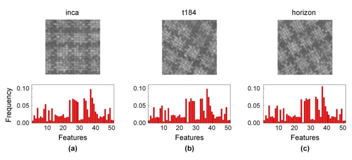
Canvas005 texture images and their histograms using discriminative features. texture images were acquired under illumination (a) “inca” at 0° rotation, (b) “t184” at 30° rotation, and (c) “horizon” at 60° rotation. The discriminative features were obtained from the three descriptors (LBP, VAR, and 2nd order LDDP) and two neighborhood topologies (P, R) = {(16, 2), (24, 3)}.
Table 3.
51 discriminative features from LBP, VAR, and 2nd order LDDP descriptors using two neighborhood topologies (P, R) = {(16, 2), (24, 3)}.
| Descriptor | Count | |
|---|---|---|
|
|
6 | |
|
|
9 | |
| VAR16,2 | 4 | |
| VAR24,3 | 3 | |
|
|
5 | |
|
|
9 | |
|
|
1 | |
|
|
1 | |
|
|
1 | |
|
|
5 | |
|
|
3 | |
| VAR16,2 + VAR24,3 | 3 | |
|
|
1 |
5.2. Experiments on CUReT Database
Here, we learned the classification models on the training dataset of 2135 images and tested on the validation dataset of 5063 images. The classification performance of our approach outperformed the conventional approach (Table 4). The highest accuracies of 79.12% (correlation) and 79.10% (cosine) were achieved. The improvement was shown for the most of the 77 combinations of the descriptors and spatial resolutions (correlation; >92% and cosine; >89%). On average, the classification accuracy increased by ~5% for the two distance metrics. The results demonstrate the robustness of our approach to differing viewing angles and illumination orientations. Moreover, the (average) number of discriminative features was substantially small (correlation; 449 and cosine; 421) compared to the conventional classification method.
Table 4.
Classification performance (%) on CUReT dataset.
| (8,1) | (16,2) | (24,3) | (8,1)+(16,2) | (8,1)+(24,3) | (16,2)+(24,3) | (8,1)+(16,2)+(24,3) | ||||||||
|---|---|---|---|---|---|---|---|---|---|---|---|---|---|---|
|
| ||||||||||||||
| dCOR | WHOLE | FP | WHOLE | FP | WHOLE | FP | WHOLE | FP | WHOLE | FP | WHOLE | FP | WHOLE | FP |
| LBP | 53.68 | 58.8 | 60.34 | 58.33 | 58.33 | 57.87 | 69.13 | 71.16 | 70.79 | 73.51 | 69.82 | 67.47 | 73.02 | 74.09 |
| VAR | 35.20 | 35.20 | 33.42 | 33.42 | 31.60 | 31.60 | 47.54 | 50.05 | 48.29 | 50.39 | 39.8 | 43.77 | 48.31 | 52.06 |
| LDDP2 | 41.04 | 51.87 | 48.00 | 55.13 | 54.02 | 56.23 | 65.00 | 69.58 | 67.47 | 71.30 | 63.54 | 66.27 | 69.82 | 73.71 |
| LDDP3 | 28.97 | 44.38 | 38.24 | 45.66 | 40.11 | 43.91 | 50.05 | 58.6 | 56.43 | 60.75 | 54.63 | 59.19 | 59.00 | 65.28 |
| LBP/VAR | 62.67 | 63.76 | 59.02 | 60.95 | 48.75 | 52.74 | 64.37 | 70.31 | 60.85 | 68.06 | 56.73 | 67.25 | 61.72 | 72.23 |
| LBP/LDDP2 | 72.66 | 72.96 | 71.32 | 70.35 | 65.2 | 67.63 | 76.28 | 76.93 | 77.17 | 78.45 | 71.91 | 74.01 | 76.85 | 79.12 |
| LBP/LDDP3 | 66.82 | 68.81 | 67.49 | 69.64 | 66.03 | 68.48 | 74.28 | 75.29 | 75.71 | 76.91 | 71.91 | 74.84 | 76.02 | 77.86 |
| VAR/LDDP2 | 56.47 | 56.37 | 53.53 | 55.54 | 43.61 | 51.79 | 59.43 | 65.28 | 55.92 | 63.46 | 52.34 | 62.08 | 57.14 | 68.34 |
| VAR/LDDP3 | 48.00 | 51.51 | 42.80 | 46.95 | 36.46 | 41.50 | 50.60 | 56.05 | 49.12 | 56.23 | 44.84 | 51.27 | 49.48 | 56.19 |
| LBP/VAR/LDDP2 | 68.44 | 69.62 | 58.82 | 67.57 | 47.48 | 62.18 | 64.68 | 72.61 | 57.44 | 73.24 | 55.34 | 73.75 | 59.35 | 75.92 |
| LBP/VAR/LDDP3 | 66.30 | 65.28 | 58.19 | 64.57 | 47.05 | 60.28 | 63.32 | 71.40 | 56.43 | 71.34 | 55.16 | 73.55 | 58.34 | 73.97 |
|
| ||||||||||||||
| COS | WHOLE | FP | WHOLE | FP | WHOLE | FP | WHOLE | FP | WHOLE | FP | WHOLE | FP | WHOLE | FP |
|
| ||||||||||||||
| LBP | 57.52 | 58.8 | 63.64 | 58.8 | 63.93 | 58.34 | 69.27 | 71.16 | 71.38 | 73.53 | 69.48 | 67.63 | 72.92 | 74.26 |
| VAR | 38.49 | 38.49 | 35.81 | 35.81 | 32.81 | 32.81 | 48.31 | 50.37 | 49.28 | 50.54 | 40.59 | 43.53 | 48.86 | 52.24 |
| LDDP2 | 46.45 | 53.84 | 52.95 | 55.82 | 58.9 | 56.51 | 64.17 | 69.35 | 67.37 | 71.52 | 63.20 | 66.30 | 69.05 | 73.47 |
| LDDP3 | 34.94 | 45.13 | 41.67 | 47.94 | 49.81 | 45.03 | 50.72 | 58.76 | 56.39 | 61.39 | 53.90 | 60.26 | 58.21 | 65.08 |
| LBP/VAR | 63.72 | 63.93 | 59.65 | 61.29 | 49.50 | 54.12 | 65.00 | 70.65 | 60.83 | 68.36 | 57.06 | 67.35 | 61.76 | 72.23 |
| LBP/LDDP2 | 72.84 | 72.96 | 71.03 | 70.29 | 65.30 | 67.49 | 76.08 | 76.91 | 77.19 | 78.47 | 71.85 | 73.97 | 76.81 | 79.10 |
| LBP/LDDP3 | 67.37 | 68.64 | 67.67 | 69.78 | 66.42 | 68.73 | 74.05 | 75.31 | 75.73 | 76.91 | 71.72 | 74.86 | 76.00 | 77.88 |
| VAR/LDDP2 | 57.50 | 56.35 | 54.04 | 55.68 | 44.68 | 53.98 | 59.63 | 65.81 | 56.17 | 66.09 | 52.72 | 61.80 | 57.02 | 68.89 |
| VAR/LDDP3 | 48.65 | 51.47 | 43.33 | 47.11 | 36.86 | 41.99 | 50.86 | 56.09 | 49.40 | 56.29 | 45.13 | 51.31 | 49.67 | 58.88 |
| LBP/VAR/LDDP2 | 68.85 | 69.56 | 59.47 | 66.66 | 48.00 | 63.54 | 65.14 | 73.18 | 57.54 | 73.63 | 55.62 | 73.77 | 59.57 | 75.75 |
| LBP/VAR/LDDP3 | 66.07 | 66.40 | 58.6 | 63.99 | 47.32 | 62.65 | 63.40 | 71.60 | 56.49 | 71.42 | 55.38 | 72.96 | 58.42 | 73.87 |
WHOLE and FP represent the conventional classification approach and our framework of using frequent pattern mining and feature selection, respectively. dCOR and COS are correlation and cosine distance metric, respectively. (P, R) indicates neighborhood topology. LDDP2 and LDDP3 denote 2nd and 3rd order LDDP, respectively. WHOLE uses rotation invariant uniform pattern codes and FP adopts rotation invariant pattern codes. Bold indicates the highest accuracy in the experiment. / and + denote a joint histogram and a concatenation of multiple histgorams, respectively.
5.3. Robustness to parameters
We repeated the above experiments using different parameter values in discovering discriminative features and classifying images (Figure 5). We first changed the number of nearest neighbors (k=1,5,10) in assigning a class to a test image. Increasing the number of nearest neighbors, the accuracies, in general, dropped for both the conventional approach and our approach; however, our approach constantly outperformed the conventional approach for both Outex and CUReT datasets. We also changed MINSUP (1%, 0.5%, 0.2%, and 0.1%) in extracting frequent patterns. Varying MINSUP, our classification performance was consistent and superior to the conventional approach regardless of the datasets. Moreover, the results were comparable between correlation and cosine distance metrics. Hence, these experiments ensure the robustness of our approach to the parameter values and the choice of a distance metric.
Figure 5.

Classification performances for different parameter values and distance metrics. Our framework is consistently superior to the conventional classification approach (WHOLE) as varying the number of nearest neighbors (k), minimum support (MINSUP) for frequent pattern mining, and distance metrics (a) Correlation and (b) Cosine. AVG and MAX represent the average and highest classification accuracies, respectively.
6. CONCLUSIONS
We have presented an efficient data mining framework for LBP and its variants in texture image analysis. Frequent pattern mining and mutual information-based feature selection could provide useful and discriminative features for the analysis. Improvement over the conventional classification approach on the two comprehensive texture databases confirms the robustness and utility of our approach. The approach is generic and straightforward to apply for other applications.
The experimental results showed that our approach could efficiently and effectively find a smaller number of discriminative features that are on average 5- to 10-fold fewer than the conventional approach. In the experiments, a limited number of combinations were tested due to the time- and space-complexity. Suppose that three descriptors (LBP, VAR, and LDDP) and two neighborhood topologies (P, R) = {(16,2), (24,3)} are incorporated. There are (3×2)!=720 possible combinations of the descriptors and the total dimensionality would be >50 million. This is impractical and intractable with the conventional approach. However, our approach found 51 discriminative features including 13 different combinations of the descriptors. Even, these 13 combinations generate a huge feature space with the conventional approach. Although various combinations of the descriptors are utilized, the computational complexity of our approach in a testing phase was comparable to the conventional approach.
LBP has been extensively studied. Thresholding and/or encoding scheme (Rassem & Khoo, 2014) (Song & Yan, 2014) and neighborhood topology (Y. G. He & Sang, 2013) have been improved. Other variants include multi-scale approaches (Xiaofei, et al., 2013) (Li, et al., 2015), feature selection methods (Girish, et al., 2014), and noise-resistant approaches (Chen, et al., 2013) (Ren, Jiang, & Yuan, 2013) (Ziqi, et al., 2014). LBP has been also combined with other texture descriptors (Shufu, Shiguang, Xilin, & Wen, 2008) (Zhe, Hong, Yueliang, & Tao, 2012) (M. Zhang, Muramatsu, Zhou, Hara, & Fujita, 2015). Each of these variants has its own advantages and disadvantages. Combining complementary variants may further improve their capability. However, how to choose the proper LBP variants and how to combine them has not been explicitly studied yet. In our approach, the informative features for texture image analysis are discriminative as well as frequent. Introducing the concept of “frequent pattern”, we efficiently and effectively explore the high dimensional feature space and reduce the dimensionality to a manageable size. Frequent patterns can be any combination of the descriptors that are incorporated in the analysis. Non-frequent patterns generate noisy features and thus deteriorate the analysis. Employing frequent pattern mining, we not only avoid the vast amount of noisy features but also examine various combinations of the descriptors and select the adequate combinations for the analysis. Therefore, our approach seeks to find the most informative combinations of the descriptors and their binary pattern codes for texture image analysis. Any LBP variant and feature selection method could potentially benefit from frequent pattern mining.
This study provides some insightful and practical implications for texture image analysis. In texture image analysis, it is not only how to characterize texture images but also how to select the informative features that determines the performance of the analysis. Except LBP, there are many types of feature descriptors such as Gabor filtering, co-occurrence matrix, wavelet transform, scale-invariant feature transform (SIFT), and histogram of gradients (HOG). Similar to LBP and its variants, combining such descriptors could improve the texture analysis. Frequent pattern mining may provide an efficient and effective manner to examine them.
There are several limitations to this study. First, our approach requires a training phase. Depending on the size of dataset and parameter settings, the training time could vary from a few minutes to hours. However, in a testing phase, its time and computational complexity is comparable to the conventional approach due to the (relatively) smaller size of the discriminative feature set. Second, our approach introduces an additional user-specified parameter, so called minimum support (MINSUP). Since the parameter determines the initial set of frequent patterns, it affects the training time and the classification performance. Although the experimental results showed that the classification performance is robust to the change in the minimum support, the optimal value is not clear a priori. Third, we validated our approach on the two texture image databases. There are a variety of databases and further validation on them would further confirm the robustness of our approach. Fourth, three texture descriptors (LBP, VAR and LDDP) were considered in this study. Other variants of LBP can also be incorporated. Last, although our approach outperformed the conventional approach, the meaning of the discriminative features is not yet clear. Further studies should be followed to examine the discriminative features in detail.
We propose the following future research directions. The first direction is to further examine the discriminative features in the texture images. The discriminative features can be mapped back to the images so that we can not only visualize the features but also analyze the chosen regions to better understand the textures. The second direction is to optimize the parameters in our approach. MINSUP, in particular, needs to be further studied. The third direction is to incorporate other feature selection schemes. Both linear and non-linear feature selection methods could be applicable. The fourth direction is to incorporate other variants of LBP and examine their relationships in texture analysis. The fifth direction is to apply our approach to more applications; for example, object recognition, image retrieval, and medical image analysis.
Highlights.
Improve the performance of local binary pattern in texture image analysis
Frequent pattern mining efficiently explores the high-dimensional feature space
Mutual information-based feature selection selects the most discriminative features
Maintains low computational complexity
Acknowledgments
This work was supported by the Intramural Research Program of the National Institutes of Health. This study utilized the high-performance computational capabilities of the Biowulf Linux cluster at the National Institutes of Health, Bethesda, MD. (http:/biowulf.nih.gov).
Footnotes
Publisher's Disclaimer: This is a PDF file of an unedited manuscript that has been accepted for publication. As a service to our customers we are providing this early version of the manuscript. The manuscript will undergo copyediting, typesetting, and review of the resulting proof before it is published in its final citable form. Please note that during the production process errors may be discovered which could affect the content, and all legal disclaimers that apply to the journal pertain.
Contributor Information
Jin Tae Kwak, Email: jintae.kwak@nih.gov.
Sheng Xu, Email: xus2@cc.nih.gov.
Bradford J. Wood, Email: bwood@cc.nih.gov.
References
- Ahonen T, Hadid A, Pietikainen M. Face description with local binary patterns: application to face recognition. IEEE Trans Pattern Anal Mach Intell. 2006;28:2037–2041. doi: 10.1109/TPAMI.2006.244. [DOI] [PubMed] [Google Scholar]
- Bovik AC, Clark M, Geisler WS. Multichannel texture analysis using localized spatial filters. Pattern Analysis and Machine Intelligence, IEEE Transactions on. 1990;12:55–73. [Google Scholar]
- Castellano G, Bonilha L, Li LM, Cendes F. Texture analysis of medical images. Clin Radiol. 2004;59:1061–1069. doi: 10.1016/j.crad.2004.07.008. [DOI] [PubMed] [Google Scholar]
- Chan C-H, Kittler J, Messer K. Multispectral local binary pattern histogram for component-based color face verification. Biometrics: Theory, Applications, and Systems; 2007. BTAS 2007. First IEEE International Conference on; IEEE; 2007. pp. 1–7. [Google Scholar]
- Chen J, Kellokumpu V, Zhao GY, Pietikainen M. RLBP: Robust Local Binary Pattern. Proceedings of the British Machine Vision Conference; 2013..2013. [Google Scholar]
- Cross GR, Jain AK. Markov random field texture models. Pattern Analysis and Machine Intelligence, IEEE Transactions on. 1983:25–39. doi: 10.1109/tpami.1983.4767341. [DOI] [PubMed] [Google Scholar]
- Dana KJ, Van Ginneken B, Nayar SK, Koenderink JJ. Reflectance and texture of real-world surfaces. ACM Transactions on Graphics (TOG) 1999;18:1–34. [Google Scholar]
- Etemad K, Chellappa R. Discriminant analysis for recognition of human face images. JOSA A. 1997;14:1724–1733. [Google Scholar]
- Fu X, Wei W. Centralized binary patterns embedded with image Euclidean distance for facial expression recognition. Natural Computation, 2008; ICNC’08. Fourth International Conference on; IEEE; 2008. pp. 115–119. [Google Scholar]
- Ghahramani M, Zhao GY, Pietikainen M. Incorporating Texture Intensity Information into LBP-Based Operators. Image Analysis, Scia 2013. 2013;7944:66–75. [Google Scholar]
- Girish GN, Shrinivasa Naika CL, Das PK. Face recognition using MB-LBP and PCA: A comparative study. Computer Communication and Informatics (ICCCI); 2014 International Conference on; 2014. pp. 1–6. [Google Scholar]
- Guo Y, Zhao G, Pietikäinen M, Xu Z. Computer Vision–ACCV 2010. Springer; 2011. Descriptor learning based on fisher separation criterion for texture classification; pp. 185–198. [Google Scholar]
- Guo Z, Li Q, You J, Zhang D, Liu W. Local directional derivative pattern for rotation invariant texture classification. Neural Computing and Applications. 2012;21:1893–1904. [Google Scholar]
- Guo Z, Zhang L, Zhang D. A completed modeling of local binary pattern operator for texture classification. IEEE Trans Image Process. 2010;19:1657–1663. doi: 10.1109/TIP.2010.2044957. [DOI] [PubMed] [Google Scholar]
- Guo Z, Zhang L, Zhang D, Mou X. Hierarchical multiscale LBP for face and palmprint recognition. Image Processing (ICIP); 2010 17th IEEE International Conference on; IEEE; 2010. pp. 4521–4524. [Google Scholar]
- Guo Z, Zhang L, Zhang D, Zhang S. Rotation invariant texture classification using adaptive LBP with directional statistical features. Image Processing (ICIP), 2010 17th IEEE International Conference on; IEEE; 2010. pp. 285–288. [Google Scholar]
- Han J, Cheng H, Xin D, Yan X. Frequent pattern mining: current status and future directions. Data Mining and Knowledge Discovery. 2007;15:55–86. [Google Scholar]
- Han J, Pei J, Yin Y. ACM SIGMOD Record. Vol. 29. ACM; 2000. Mining frequent patterns without candidate generation; pp. 1–12. [Google Scholar]
- Haralick RM, Shanmugam K, Dinstein IH. Textural features for image classification. Systems, Man and Cybernetics, IEEE Transactions on. 1973:610–621. [Google Scholar]
- He Y, Sang N, Gao C. Computer Vision–ACCV 2010. Springer; 2011. Pyramid-based multi-structure local binary pattern for texture classification; pp. 133–144. [Google Scholar]
- He YG, Sang N. Multi-ring local binary patterns for rotation invariant texture classification. Neural Computing & Applications. 2013;22:793–802. [Google Scholar]
- Howarth P, Rüger S. Robust texture features for still-image retrieval. IEE Proceedings-Vision, Image and Signal Processing. 2005;152:868–874. [Google Scholar]
- Hussain SU, Triggs W. Feature sets and dimensionality reduction for visual object detection. British Machine Vision Conference..2010. [Google Scholar]
- Iakovidis DK, Keramidas EG, Maroulis D. Image Analysis and Recognition. Springer; 2008. Fuzzy local binary patterns for ultrasound texture characterization; pp. 750–759. [Google Scholar]
- Jin H, Liu Q, Lu H, Tong X. Face detection using improved LBP under bayesian framework. Image and Graphics, 2004. Proceedings. Third International Conference on; IEEE; 2004. pp. 306–309. [Google Scholar]
- Khellah FM. Texture Classification Using Dominant Neighborhood Structure. Ieee Transactions on Image Processing. 2011;20:3270–3279. doi: 10.1109/TIP.2011.2143422. [DOI] [PubMed] [Google Scholar]
- Laine A, Fan J. Texture classification by wavelet packet signatures. Pattern Analysis and Machine Intelligence, IEEE Transactions on. 1993;15:1186–1191. [Google Scholar]
- Li XL, Ruan QQ, Jin Y, An GY, Zhao RZ. Fully automatic 3D facial expression recognition using polytypic multi-block local binary patterns. Signal Processing. 2015;108:297–308. [Google Scholar]
- Liao S, Chung AC. Computer Vision–ACCV 2007. Springer; 2007. Face recognition by using elongated local binary patterns with average maximum distance gradient magnitude; pp. 672–679. [Google Scholar]
- Liao S, Law MW, Chung AC. Dominant local binary patterns for texture classification. IEEE Trans Image Process. 2009;18:1107–1118. doi: 10.1109/TIP.2009.2015682. [DOI] [PubMed] [Google Scholar]
- Liao S, Zhu X, Lei Z, Zhang L, Li SZ. Advances in Biometrics. Springer; 2007. Learning multi-scale block local binary patterns for face recognition; pp. 828–837. [Google Scholar]
- Lumini LNSBA. Selecting the best performing rotation invariant patterns in local binary/ternary patterns. Int’l Conf. IP, Comp. Vision, and Pattern Recognition..2010. [Google Scholar]
- Mäenpää T, Pietikäinen M. Image Analysis. Springer; 2003. Multi-scale binary patterns for texture analysis; pp. 885–892. [Google Scholar]
- Malik J, Belongie S, Leung T, Shi J. Contour and texture analysis for image segmentation. International journal of computer vision. 2001;43:7–27. [Google Scholar]
- Manjunath BS, Ma WY. Texture features for browsing and retrieval of image data. Pattern Analysis and Machine Intelligence, IEEE Transactions on. 1996;18:837–842. [Google Scholar]
- Nanni L, Lumini A, Brahnam S. Local binary patterns variants as texture descriptors for medical image analysis. Artificial intelligence in medicine. 2010;49:117–125. doi: 10.1016/j.artmed.2010.02.006. [DOI] [PubMed] [Google Scholar]
- Nanni L, Lumini A, Brahnam S. Survey on LBP based texture descriptors for image classification. Expert Systems with Applications. 2012;39:3634–3641. [Google Scholar]
- Ojala T, Maenpaa T, Pietikainen M, Viertola J, Kyllonen J, Huovinen S. Outex-new framework for empirical evaluation of texture analysis algorithms. Pattern Recognition, 2002. Proceedings. 16th International Conference on; IEEE; 2002. pp. 701–706. [Google Scholar]
- Ojala T, Pietikainen M, Maenpaa T. Multiresolution gray-scale and rotation invariant texture classification with local binary patterns. Pattern Analysis and Machine Intelligence, IEEE Transactions on. 2002;24:971–987. [Google Scholar]
- Peng H, Long F, Ding C. Feature selection based on mutual information criteria of max-dependency, max-relevance, and min-redundancy. Pattern Analysis and Machine Intelligence, IEEE Transactions on. 2005;27:1226–1238. doi: 10.1109/TPAMI.2005.159. [DOI] [PubMed] [Google Scholar]
- Petpon A, Srisuk S. Face recognition with local line binary pattern. Image and Graphics, 2009. ICIG’09. Fifth International Conference on; IEEE; 2009. pp. 533–539. [Google Scholar]
- Rassem TH, Khoo BE. Completed Local Ternary Pattern for Rotation Invariant Texture Classification. Scientific World Journal. 2014 doi: 10.1155/2014/373254. [DOI] [PMC free article] [PubMed] [Google Scholar]
- Ren JF, Jiang XD, Yuan JS. Noise-Resistant Local Binary Pattern With an Embedded Error-Correction Mechanism. Ieee Transactions on Image Processing. 2013;22:4049–4060. doi: 10.1109/TIP.2013.2268976. [DOI] [PubMed] [Google Scholar]
- Samal A, Brandle JR, Zhang DS. Texture as the basis for individual tree identification. Information Sciences. 2006;176:565–576. [Google Scholar]
- Shan C, Gong S, McOwan PW. Computer Vision in Human-Computer Interaction. Springer; 2005. Appearance manifold of facial expression; pp. 221–230. [Google Scholar]
- Shan C, Gritti T. Learning Discriminative LBP-Histogram Bins for Facial Expression Recognition. BMVC. 2008:1–10. [Google Scholar]
- Shan S, Zhang W, Su Y, Chen X, Gao W. Ensemble of piecewise FDA based on spatial histograms of local (Gabor) binary patterns for face recognition. Pattern Recognition, 2006; ICPR 2006. 18th International Conference on; IEEE; 2006. pp. 606–609. [Google Scholar]
- Shrivastava N, Tyagi V. An effective scheme for image texture classification based on binary local structure pattern. Visual Computer. 2014;30:1223–1232. [Google Scholar]
- Shufu X, Shiguang S, Xilin C, Wen G. V-LGBP: Volume based local Gabor binary patterns for face representation and recognition. Pattern Recognition, 2008; ICPR 2008. 19th International Conference on; 2008. pp. 1–4. [Google Scholar]
- Smith RS, Windeatt T. Facial Expression Detection using Filtered Local Binary Pattern Features with ECOC Classifiers and Platt Scaling. Journal of Machine Learning Research. 2010:111–118. [Google Scholar]
- Song KC, Yan YH. Neighborhood Estimated Local Binary Patterns for Texture Classification. Applied Mechanics and Materials. 2014;513:4401–4406. [Google Scholar]
- Székely GJ, Rizzo ML, Bakirov NK. Measuring and testing dependence by correlation of distances. The Annals of Statistics. 2007;35:2769–2794. [Google Scholar]
- Tajeripour F, Kabir E, Sheikhi A. Fabric defect detection using modified local binary patterns. EURASIP Journal on Advances in Signal Processing. 2008;2008:60. [Google Scholar]
- Tan X, Triggs B. Analysis and Modeling of Faces and Gestures. Springer; 2007. Enhanced local texture feature sets for face recognition under difficult lighting conditions; pp. 168–182. [DOI] [PubMed] [Google Scholar]
- Topi M, Timo O, Matti P, Maricor S. Robust texture classification by subsets of local binary patterns. Pattern Recognition, 2000; Proceedings. 15th International Conference on; IEEE; 2000. pp. 935–938. [Google Scholar]
- Turk M, Pentland A. Eigenfaces for recognition. Journal of cognitive neuroscience. 1991;3:71–86. doi: 10.1162/jocn.1991.3.1.71. [DOI] [PubMed] [Google Scholar]
- Turtinen M, Pietikäinen M. BMVC. Citeseer; 2006. Contextual analysis of textured scene images; pp. 849–858. [Google Scholar]
- Wang X, Gong H, Zhang H, Li B, Zhuang Z. Palmprint identification using boosting local binary pattern. Pattern Recognition, 2006; ICPR 2006. 18th International Conference on; IEEE; 2006. pp. 503–506. [Google Scholar]
- Wolf L, Hassner T, Taigman Y. Descriptor based methods in the wild. Workshop on Faces in ‘Real-Life’ Images: Detection, Alignment, and Recognition 2008 [Google Scholar]
- Xiaofei J, Xin Y, Yali Z, Ning Z, Ruwei D, Jie T, Jianmin Z. Multi-scale block local ternary patterns for fingerprints vitality detection. Biometrics (ICB); 2013 International Conference on; 2013. pp. 1–6. [Google Scholar]
- Yang H, Wang Y. A LBP-based face recognition method with hamming distance constraint. Image and Graphics, 2007; ICIG 2007. Fourth International Conference on; IEEE; 2007. pp. 645–649. [Google Scholar]
- Zhang B, Gao Y, Zhao S, Liu J. Local derivative pattern versus local binary pattern: face recognition with high-order local pattern descriptor. Image Processing, IEEE Transactions on. 2010;19:533–544. doi: 10.1109/TIP.2009.2035882. [DOI] [PubMed] [Google Scholar]
- Zhang G, Huang X, Li SZ, Wang Y, Wu X. Advances in biometric person authentication. Springer; 2005. Boosting local binary pattern (LBP)-based face recognition; pp. 179–186. [Google Scholar]
- Zhang M, Muramatsu C, Zhou XR, Hara T, Fujita H. Blind Image Quality Assessment Using the Joint Statistics of Generalized Local Binary Pattern. Ieee Signal Processing Letters. 2015;22:207–210. [Google Scholar]
- Zhao D, Lin Z, Tang X. Laplacian PCA and its applications. Computer Vision, 2007; ICCV 2007. IEEE 11th International Conference on; IEEE; 2007. pp. 1–8. [Google Scholar]
- Zhao G, Pietikainen M. Local binary pattern descriptors for dynamic texture recognition. Pattern Recognition, 2006; ICPR 2006. 18th International Conference on; IEEE; 2006. pp. 211–214. [Google Scholar]
- Zhao Y, Huang DS, Jia W. Completed Local Binary Count for Rotation Invariant Texture Classification. Ieee Transactions on Image Processing. 2012;21:4492–4497. doi: 10.1109/TIP.2012.2204271. [DOI] [PubMed] [Google Scholar]
- Zhao Y, Jia W, Hu RX, Min H. Completed robust local binary pattern for texture classification. Neurocomputing. 2013;106:68–76. [Google Scholar]
- Zhe W, Hong L, Yueliang Q, Tao X. Crowd Density Estimation Based on Local Binary Pattern Co-Occurrence Matrix. Multimedia and Expo Workshops (ICMEW), 2012 IEEE International Conference on; 2012. pp. 372–377. [Google Scholar]
- Zhou H, Wang R, Wang C. A novel extended local-binary-pattern operator for texture analysis. Information Sciences. 2008;178:4314–4325. [Google Scholar]
- Zhu C, Yang X. Study of remote sensing image texture analysis and classification using wavelet. International Journal of Remote Sensing. 1998;19:3197–3203. [Google Scholar]
- Zhu CR, Wang RS. Local multiple patterns based multiresolution gray-scale and rotation invariant texture classification. I Sciences. 2012;187:93–108. [Google Scholar]
- Ziqi Z, Xinge Y, Chen CLP, Dacheng T, Xiubao J, Fanyu Y, Jixing Z. A Noise-Robust Adaptive Hybrid Pattern for Texture Classification. Pattern Recognition (ICPR), 2014 22nd International Conference on; 2014. pp. 1633–1638. [Google Scholar]