Functional mapping of the magnocellular and parvocellular subdivisions of human LGN

Abstract

The magnocellular (M) and parvocellular (P) subdivisions of primate LGN are known to process complementary types of visual stimulus information, but a method for noninvasively defining these subdivisions in humans has proven elusive. As a result, the functional roles of these subdivisions in humans have not been investigated physiologically. To functionally map the M and P subdivisions of human LGN, we used high-resolution fMRI at high field (7T and 3T) together with a combination of spatial, temporal, luminance, and chromatic stimulus manipulations. We found that stimulus factors that differentially drive magnocellular and parvocellular neurons in primate LGN also elicit differential BOLD fMRI responses in human LGN and that these responses exhibit a spatial organization consistent with the known anatomical organization of the M and P subdivisions. In test-retest studies, the relative responses of individual voxels to M-type and P-type stimuli were reliable across scanning sessions on separate days and across sessions at different field strengths. The ability to functionally identify magnocellular and parvocellular regions of human LGN with fMRI opens possibilities for investigating the functions of these subdivisions in human visual perception, in patient populations with suspected abnormalities in one of these subdivisions, and in visual cortical processing streams arising from parallel thalamocortical pathways.

Introduction

Parallel processing, the simultaneous analysis of different sensory features in different brain areas, enables the efficient representation of a huge variety of sensory properties (Nassi and Callaway, 2009). An important early site of parallel processing in the mammalian visual system is the lateral geniculate nucleus (LGN) of the thalamus, the primary thalamic relay between the retina and visual cortex (Sherman and Guillery, 2006). In primates, the LGN is composed of magnocellular (M), parvocellular (P), and koniocellular (K) layers. Monkey electrophysiological studies have demonstrated that M and P neurons, which dominate primate vision (Nassi and Callaway, 2009; Schiller et al., 1990), have distinct and complementary spatial, temporal, luminance, and chromatic stimulus preferences (Derrington and Lennie, 1984; Hicks et al., 1983; Hubel and Livingstone, 1990; Kaplan and Shapley, 1982; Reid and Shapley, 2002; Schiller and Malpeli, 1978; Shapley, 1990) as well as response dynamics (Maunsell et al., 1999; Schiller and Malpeli, 1978). As a result, M neurons are well suited for the detection of motion and other rapid visual changes occurring at large spatial scales, while P neurons are well suited for detailed form and color processing.

Although the functions of the M and P subdivisions have been well characterized in the macaque monkey LGN, their study in the human LGN has proven challenging. In particular, the LGN's small size and location deep within the brain have made it difficult to measure distinct signals from the M and P subdivisions using noninvasive techniques. However, there are strong motivations to study these subdivisions in humans, including: understanding their roles in human visual perception, attention, and awareness (Denison and Silver, 2012; Livingstone and Hubel, 1988; Yeshurun and Levy, 2003); characterizing their interactions with large-scale cortical networks; and evaluating their involvement in human disorders such as dyslexia (Stein and Walsh, 1997) and schizophrenia (Butler and Javitt, 2005). Moreover, given the lack of functional data from human M and P subdivisions, the degree to which their functional properties have been conserved across humans and other primates remains an open question. While conservation is expected based on similarities in both visual system anatomy and visual perception between monkeys and humans (de Courten and Garey, 1982; De Valois et al., 1974a; De Valois et al., 1974b; Merigan, 1989; see Livingstone and Hubel, 1988; Livingstone and Hubel, 1987), perfect homology between the species cannot be assumed (Hickey and Guillery, 1979).

Here we report the first robust demonstration of functional maps of the M and P subdivisions of human LGN using fMRI at 7T and 3T, employing stimuli based on the response properties of monkey M and P neurons. Maps with anatomically correct spatial organization were observed in nearly all hemispheres, and individual subjects' maps were reliable across separate scanning sessions.

Material and Methods

Subjects

Six adult subjects (25-27 years of age; 1 male, 5 females) participated in the study. Three subjects were scanned in multiple sessions, and two of the subjects were authors. All subjects provided written informed consent, and all experimental protocols were approved by the Committee for the Protection of Human Subjects at the University of California, Berkeley, or the Institutional Review Board for human subjects research at the University of Minnesota, as appropriate. Subjects had normal or corrected-to-normal visual acuity.

Visual display

The stimuli were generated on Macintosh computers using MATLAB (The MathWorks Inc., Natick, MA), Psychophysics Toolbox (Brainard, 1997; Pelli, 1997), and Python with Vision Egg (Straw, 2008) and displayed using gamma-corrected projection systems. In Minnesota, stimuli were projected from a NEC NP4000 (NEC Display Solutions, Tokyo) liquid crystal display projector located outside the scanner room and reflected via a mirror onto a translucent screen positioned over the subject's chest. The screen was viewed via a mirror mounted over the subject's eyes, with a total viewing distance of 23-31 cm. The screen height subtended 20-29 degrees of visual angle, and the screen width subtended 47-70 degrees of visual angle, with variability across subjects arising from differences in screen positioning. In Berkeley, stimuli were projected from an Avotec SV-6011 (Avotec, Inc., Stuart, FL) liquid crystal display projector onto a translucent screen located at the end of the scanner bore behind the subject's head. The screen was viewed via a mirror mounted over the subject's eyes, with a total viewing distance of 29 cm. The screen height subtended 34-37 degrees of visual angle, and the screen width subtended 44-48 degrees of visual angle.

Visual stimulus

An alternating hemifield stimulus (Figure 1A) was used to localize the LGN (Figure 1B). This stimulus consisted of a 100% contrast flickering checkerboard pattern that reversed contrast polarity at a frequency of 4 Hz (for the full flicker cycle). This checkerboard had a radial check pattern with a check size of 15° polar angle and an eccentricity that was scaled according to the formula s = 0.05 × r^0.8, where s is check size and r is distance from fixation in degrees of visual angle. The checkerboard pattern covered half of the screen except for the central 0.6° of visual angle, which contained background gray luminance (50% contrast, luminance 105 cd/m² (3T) or 1019 cd/m² (7T)). The other half of the screen also contained the gray background. A white fixation point subtending 0.2° of visual angle appeared at the center of the screen throughout the run, and subjects were instructed to maintain fixation while passively viewing the stimuli. For each run, the checkerboard pattern alternated between the left and right halves of the screen, 16 s (7T) or 13.5 s (3T) per side, and was presented for 8 (7T) or 11 (3T) left-right cycles.

Figure 1.

LGN M/P localization methods. (A) A flickering checkerboard stimulus that alternated between the left and right visual hemifields was used to localize the LGN. (B) Voxels were selected that responded selectively to contralateral visual field stimulation. Coherence threshold = 0.19 in this example (see Material and Methods). LGN regions are indicated by white circles. (C) M-type (monochrome, low spatial frequency, high temporal frequency, high luminance contrast) and P-type (high color contrast, high spatial frequency, low temporal frequency, low luminance contrast) grating stimuli were designed to elicit differential BOLD responses from the M and P subdivisions of human LGN. Subjects maintained fixation at the center of the screen while viewing blocks of full-field M and P stimuli that were interleaved with blocks of blank stimuli. Concurrently, subjects performed a contrast decrement detection task during the M- and P-stimulus blocks, counting the number of luminance contrast (M blocks) or color contrast (P blocks) targets that appeared in each block.

An M/P localizer stimulus (Figure 1C) was designed to elicit differential responses from voxels with greater M-layer representation and voxels with greater P-layer representation, based on findings from monkey electrophysiology (see Kleinschmidt et al., 1996 and Liu et al., 2006 for related approaches). The M/P localizer consisted of 16-s (7T) or 18-s (3T) blocks of “M stimuli”, “P stimuli”, and blank (fixation point only) stimuli. The M and P stimuli were both full-field sinusoidal gratings with sinusoidal counterphase flicker. The outer borders of the stimulus faded into gray to avoid sharp visual edges at the stimulus boundaries. The gratings were presented at one of 6 orientations (0°, 30°, 60°, 90°, 120°, or 150°) and changed to a new random orientation every 3 s, in order to drive different populations of LGN neurons with different spatial receptive fields throughout the block.

The M stimulus was a 100% luminance contrast, black-white grating with a spatial frequency of 0.5 cpd and a flicker frequency of 15 Hz. The P stimulus was a low luminance-contrast, high color-contrast red-green grating with a spatial frequency of 2 cpd and a flicker frequency of 5 Hz. A spatial frequency of 2 cpd was selected for the P stimulus because contrast sensitivity for isoluminant stimuli is attenuated at high spatial frequencies (De Valois and De Valois, 2000). The blank stimulus was a gray screen of mean luminance.

The red and green levels of the P stimulus were set to be near-isoluminant by performing heterochromatic flicker photometry outside the scanner. Specifically, subjects adjusted the luminance of a green disk to match a 100% red disk on a neutral gray background by minimizing the perception of flicker as the two disks alternated at a frequency of 7.5 Hz. Two subjects (S2 and S3) performed flicker photometry, and the average green value (39%) from these subjects was used for all scanning sessions.

Although we did not perform flicker photometry in the scanner for all subjects (due to time constraints as well as a concern about adapting subjects to the red and green stimuli before the M/P localizer scans), we verified that the green luminance value obtained outside the scanner was reasonable for both scanner displays by obtaining flicker photometry data from two subjects on the 7T display (mean of 41% green) and one subject on the 3T display (49% green). Since the values needed to achieve isoluminance vary across subjects and across the visual field, our main objective was to create a standard low luminance contrast stimulus that would enable relative activation of the M vs. P subdivisions.

On each run, 15 blocks (6 M, 6 P, and 3 blank) were presented in pseudorandom order, with the constraint that the same stimulus type could not appear in adjacent blocks in order to minimize adaptation to the M or P stimuli. A white fixation point subtending 0.2° visual angle appeared at the center of the screen throughout the stimulus blocks, and subjects were instructed to maintain fixation throughout the run.

Subjects performed a target detection task during the M and P stimulus blocks to encourage them to attend to the visual stimuli throughout the run (Figure 1C). Targets were contrast decrement 2-dimensional Gaussians presented for 300 ms. We used luminance contrast decrements (fade to gray) for M blocks and color contrast decrements (fade to yellow) for P blocks, since luminance contrast was already minimal for the P stimuli. Target size was linearly scaled with eccentricity by adjusting the sigma parameter of the Gaussian. The overall target size was set individually for each subject, separately for the M and P stimulus conditions, to attempt to equate task difficulty in the M and P blocks.

During each stimulus block, 0, 1, 2, or 3 targets appeared on the screen, and subjects were asked to count the number of targets in each block. Targets appeared at random times throughout the block and could appear at any location within the stimulus. At the end of a stimulus block, the screen turned gray and the fixation point turned black for 1.5 s (7T) or 1.75 s (3T), indicating the response period. During this time, subjects pressed a button to report how many targets they had seen during the previous stimulus block. The fixation point then turned white for 500 ms, indicating the start of the next stimulus block. Therefore, the total block duration (including stimulus, response, and cue periods) was 18 s (7T) or 20.25 s (3T), corresponding to 9 TRs in both cases. At the beginning of each run (before the stimulus blocks), an 8 s (7T) or 9 s (3T) blank stimulus was presented, which the subject viewed passively while maintaining fixation. In the 7T sessions, an 8-s blank stimulus was also shown at the end of each run. M/P localizer runs were about 5 minutes in length, with 4-12 (median 8) runs collected per session (Table 1).

Table 1. M/P mapping methods by session.

M/P mapping methods for each experimental session showing parameters that varied across sessions. iPAT = in-plane parallel imaging factor. MB = multiband slice parallel imaging factor. TE = echo time.

	Session	Subject	Paired sessions for cross-session reliability	Number of M/P runs	Voxel size	Matrix size	IPAT	MB	Partial Fourier	Number of slices	TE (ms)	Flip angle (deg)	Echo spacing (ms)	Notes
7T	1	1	7T 2 and 3	7	1.5 mm isotropic	128 × 128	3	-	6/8	38	18	80	0.82	-
	2	1	7T 1	4	1.5 mm isotropic	128 × 128	3	-	6/8	40	17	78	0.82	Sessions 2 and 3 were collected contiguously
	3	1	7T 1	4	1.25 × 1.25 × 1.2 mm	154 × 154	3	-	6/8	38	16	80	0.76	Sessions 2 and 3 were collected contiguously. Hemifield localizer from session 2.
	4	2	3T 1 and 2	8	1.5 mm isotropic	128 × 128	3	-	6/8	38	17	78	0.72	-
	5	3	3T 3	11	1.5 mm isotropic	128 × 128	3	-	6/8	38	18	80	0.82	12 runs were collected, but one was excluded due to an artifact
	6	4	-	8	1.3 mm isotropic	160 × 160	2	2	5/8	64	17	70	0.74	ROIs from GLM, not hemifield localizer
	7	5	-	6	1.3 mm isotropic	160 × 160	2	2	5/8	64	17	70	0.74	-
3T	1	2	7T 4, 3T 2	8	1.75 × 1.75 × 1.5 mm	128 × 128	-	-	6/8	21	40	75	0.78	-
	2	2	7T 4, 3T 1	8	1.75 × 1.75 × 1.5 mm	128 × 128	-	-	6/8	21	40	75	0.78	-
	3	3	7T 5	12	1.75 × 1.75 × 1.5 mm	128 × 128	-	-	6/8	21	40	75	0.78	-
	4	6	-	7	1.75 × 1.75 × 1.5 mm	128 × 128	-	-	6/8	21	40	75	0.78	-

MRI data acquisition

7-Tesla MRI anatomical and functional images were acquired at the University of Minnesota on a whole-body scanner driven by a Siemens console with a head RF coil (Nova Medical; single transmit, 24 receive channels). BOLD data were acquired using a T2*-weighted single-shot gradient-echo echo planar imaging sequence that included both parallel imaging and fat suppression. Slices were near axial and were oriented to cover LGN and the occipital lobe as well as parts of the parietal and temporal lobes. TR was 2000 ms, with 144 volumes acquired per run. The phase encoding direction was anterior-to-posterior, and the slice acquisition order was interleaved. Other acquisition parameters varied across sessions, as detailed in Table 1. These parameters included: parallel imaging methods (in-plane phase-encode acceleration factors (iPAT) of 2 or 3 and a multiband (MB) slice acceleration factor (Feinberg et al., 2010; Moeller et al., 2010; Setsompop et al., 2012) of 2), partial Fourier of 5/8 or 6/8, number of slices (38, 40, or 64), slice thickness (1.2-1.5 mm, 0 mm gap), in-plane resolution (1.25 × 1.25 mm – 1.5 × 1.5 mm), TE (16-18 ms), flip angle (70-80°), and echo spacing (0.72-0.82 ms). Matrix size ranged from 128 × 128 to 160 × 160, and in-plane FOVs ranged from 192 × 192 mm to 208 × 208 mm. A high-resolution T1-weighted MPRAGE anatomical volume with a spatial resolution of 1 × 1 × 1 mm was acquired for each subject, sometimes in a separate session. Subjects lay head first, supine, in the scanner, with foam padding around the head to reduce head motion.

3-Tesla MRI data were acquired at the University of California, Berkeley, using a Siemens Trio scanner equipped with a 32-channel head coil. BOLD data were acquired using a T2*-weighted single-shot gradient-echo echo planar imaging sequence with 6/8 partial Fourier acquisition and fat suppression. 21 near-axial slices (1.5 mm thickness, 0.075 mm gap) were acquired with a 128 × 128 matrix and in-plane FOV of 224 × 224 mm for a spatial resolution of 1.75 × 1.75 × 1.575 mm, covering LGN and parts of the occipital lobe, including the calcarine sulcus. TR was 2250 ms, with 139 volumes acquired per run. TE = 40 ms, flip angle = 75°, the phase encoding direction was anterior-to-posterior, and echo spacing = 0.78 ms. The slice acquisition order was interleaved. A Siemens prescan normalize filter was applied to the functional images at the time of acquisition to reduce spatial inhomogeneities. This filter normalizes the functional images by the receive field of the head RF coil, which is calculated from separate scans.

Before the 3T functional runs, 21 slices (1.5 mm thickness, 0.075 mm gap) of an in-plane anatomical volume were acquired with a 256 × 256 matrix and in-plane FOV of 225 mm × 225 mm, for a spatial resolution of 0.88 × 0.88 × 1.575 mm. This volume had the same slice thickness and positioning as the functional scans and was used to facilitate the alignment of the functional scans to a high-resolution T1-weighted MPRAGE anatomical volume with a spatial resolution of 1 × 1 × 1 mm (which was sometimes acquired in a separate session). Subjects lay head first, supine, in the scanner, with foam padding around the head to reduce head motion.

Data analysis

fMRI preprocessing

To correct for subject motion, all functional volumes from each run were aligned to the first volume of the session using FSL MCFLIRT (Jenkinson et al., 2002). The first volume was selected because it was acquired closest in time to the in-plane anatomical volume (which was collected only in 3T sessions). To assess subject head motion, we calculated the maximum translational and rotational displacements across each session from the 6 motion parameters (3 translation, 3 rotation) obtained from MCFLIRT. Total translational displacements were defined as the square root of the sum of squared x, y, and z-direction displacements. Total rotational displacements were defined as the sum of the absolute values of the rotational displacements in the three orthogonal directions. The maximum difference between these referenced displacements across the session was then calculated. Because small but frequent head motion can have different effects on data quality than large but infrequent head motion while producing similar levels of total head displacement over the course of a scan, we also calculated the mean framewise displacement (FD), which summarizes translational and rotational head motion between adjacent frames, with rotational displacements converted from degrees to mm by assuming a spherical surface with radius 50 mm (Power et al., 2012). This overestimates the rotational displacement of the LGN, since it is less than 50 mm from the center of the brain, but we used this value in order to facilitate comparison with other reports of FD. Head motion values are reported in Table 2.

Table 2. Estimated head motion.

Head motion estimates, giving the mean and range (in parentheses) of each metric across subjects. Max displacement is the difference between the two head positions that were farthest from one another during the session. FD = framewise displacement.

	Max translational displacement (mm)	Max rotational displacement (deg)	Mean FD (mm)
7T	2.8 (1.2-4.4)	2.4 (1.5-3.7)	0.12 (0.08-0.15)
3T	1.5 (0.8-2.5)	2.3 (1.7-3.0)	0.14 (0.13-0.17)

Next, volumes at the beginnings and ends of functional runs were discarded. For hemifield localizer runs, volumes corresponding to half of a stimulus alternation cycle (7T sessions 6 and 7: 8 volumes, 3T: 6 volumes) or a full alternation cycle (7T sessions 1-5: 16 volumes) were discarded from the beginning of each run. Volumes were also discarded from the ends of runs in some sessions (7T session 6: 8 volumes; session 7: 64 volumes; 3T: 1 volume). In all hemifield localizer runs, 128 volumes (7T) or 132 volumes (3T) were retained for the analysis. For M/P localizer runs, either 4 volumes at the beginning of each run (3T) or 4 volumes at the beginning and 5 volumes at the end of each run (7T) were discarded. These discarded volumes corresponded to initial and final blank periods, which were presented in addition to the three blank stimulus blocks in each M/P localization run. In all M/P localizer runs, 135 volumes were retained for analysis.

For all functional runs, the time series for each voxel was then detrended to remove low-frequency noise and slow drift (Smith et al., 1999; Zarahn et al., 1997). Finally, each voxel time series was divided by its mean to convert the arbitrary image intensity units into percent signal change.

Alignment to high-resolution anatomical

For each subject, the in-plane anatomical volume (3T) or mean volume of the first functional run (following motion correction) (7T) was aligned to the high-resolution anatomical volume through the combined use of an automatic alignment tool (Nestares and Heeger, 2000) and manual adjustment in the VISTA software package mrVista (http://white.stanford.edu/software/). Conversion of anatomical coordinates into Talairach space was performed within mrVista by selecting anatomical landmarks on the high-resolution anatomical volume and applying a coordinate transformation for each subject based on these landmarks.

LGN ROI definition

ROIs corresponding to the entire LGN (including both M and P subdivisions) were defined by identifying voxels responding to contralateral visual stimulation using Fourier analysis of the hemifield localizer runs. Coherency (coherence magnitude and phase) was calculated between the average time series of hemifield-alternation runs in each voxel and a sinusoid with a frequency equal to that of the hemifield alternation cycles.

The LGN region was identified as a cluster of voxels in the appropriate anatomical location having high coherency magnitudes and phases corresponding to contralateral visual responses. Specifically, the coherency magnitude threshold was adjusted to retain bilateral clusters of voxels with similar phases in the LGN regions while reducing the presence of noisy voxels with heterogeneous phases elsewhere. Because signal-to-noise differed across sessions, this adjustment was done separately for each session. Thresholds ranged from C>0.19 to C>0.21 for 7T sessions and from C>0.17 to C>0.19 for 3T sessions. ROI borders were manually drawn around these clusters in functional space. In uncertain cases, voxels were checked for survival across a range of thresholds. Occasionally, voxels that did not meet the threshold were included in order to preserve the convexity of the structure, with the knowledge that ROIs would be subsequently restricted based on further functional criteria.

For one session (7T session 6), the hemifield localizer runs did not have sufficiently high coherence values, perhaps due to eye movements during the runs. For this session, the LGN ROIs were defined based on the GLM analysis (see below), from the clusters of voxels for which the time series variance explained by the GLM exceeded 2%. This variance explained threshold was selected using thresholding heuristics similar to those used for setting coherence thresholds in the other sessions (i.e., to reveal bilateral LGN clusters while reducing noisy voxels elsewhere). For 7T session 3, which was conducted consecutively with session 2 (the subject remained in the scanner but was tested with different scanning parameters), a separate hemifield localizer was not collected; instead the ROIs from session 2 were used. All ROIs were defined before conducting the M/P mapping analysis.

Estimation of responses to M and P stimuli

A GLM analysis was performed to estimate the responses of each LGN voxel to M and P stimuli. A design matrix was constructed with an M regressor (1 when the M stimulus was on and zero otherwise), a P regressor (1 when the P stimulus was on and zero otherwise), and one regressor for each run (1 during a given run and zero otherwise). Each regressor was then convolved with a gamma function HRF (Boynton et al., 1996) to generate the final design matrix. This model was fit to the time series (a concatenation of all M/P runs in a session) of each voxel using mrVista. The estimated responses of each voxel to the M and P stimuli correspond to beta_M and beta_P, respectively. The relative response of each voxel to M vs. P stimuli was defined as the difference between beta_M and beta_P (beta_M-P) for that voxel. Negative beta_M or beta_P values likely indicate a poor (noisy) response to that stimulus, though in principle they could reflect suppression compared to the blank stimulus.

Spatial analyses

To quantify the spatial organization of the M/P functional maps, we divided LGN voxels into M and P groups and compared the spatial centers of the two groups. We classified each functional voxel as belonging to either the M or P group based on its beta_M-P value. Since human histological studies have found that, on average, 20% of the volume of the LGN is made up of M layers and 80% is made up of P layers (Andrews et al., 1997; Selemon and Begovic, 2007), we considered the 20% of voxels with the highest beta_M-P values to be the M group and the remaining 80% of voxels to be the P group. The 3D spatial center of each group in each LGN was defined as the mean voxel coordinate in each spatial dimension (anterior-posterior, dorsal-ventral, and medial-lateral). These center coordinates were then transformed into Talairach space to provide a unified spatial reference frame with a canonical brain orientation, which facilitated comparison across subjects.

Map consistency across thresholds

To assess map consistency across a range of voxel selection criteria, we repeated the spatial centers analysis procedure for many levels of thresholding, based on the proportion of variance explained by the GLM for each voxel. Only voxels in the LGN ROIs defined from the hemifield localizer were considered. Thresholding by proportion of variance explained is an unbiased procedure, as this measure reflects voxel responses to both M and P stimuli. Voxels that did not meet the variance explained threshold were excluded from the LGN ROI for that threshold level. We then repeated the spatial centers analysis in each ROI for each threshold level. Different threshold ranges were used for 7T (0-0.05) and 3T (0-0.01) data, due to the overall higher proportions of variance explained at 7T. Threshold levels were spaced at intervals of 0.001 proportion variance explained.

Reliability analyses

In order to assess consistency of LGN M/P maps across scans, we performed cross-session and within-session reliability analyses on the beta_M-P values for each voxel. Cross-session reliability was evaluated for M/P mapping data collected from the same individual scanned on two different days. Table 1 shows all the sessions performed in this study and lists the paired comparison sessions (if any) for each one. For subjects who participated in multiple sessions, all pairwise combinations of sessions were compared, with the exception of 7T sessions 2 and 3, since these sessions were conducted during the same scanning period (i.e., the subject was continuously in the magnet), not on separate days.

Cross-session reliability was measured as the correlation between beta_M-P maps collected from the same subject on two different days. The two beta_M-P maps were projected from functional space to an aligned high-resolution anatomical image and then resampled to the resolution of the anatomical volume using nearest neighbor interpolation. The intersection between the LGN ROIs defined from the two sessions was then computed in anatomical space. Only voxels that were common to both ROIs were considered for the reliability analysis. We then computed the Pearson correlation coefficient between the beta_M-P values from the two days. For each LGN ROI comparison pair, we calculated the proportion overlap of the two ROIs as the ratio of the volume of their intersection to the volume of their union.

Within-session reliability was defined as the inter-run correlation in beta_M-P values across voxels. Separate GLMs were performed for each M/P mapping run, resulting in separate beta_M-P estimates for each run for every voxel. The Pearson correlation of these beta_M-P values across voxels in each LGN ROI was calculated for all pairwise comparisons of runs, and the inter-run correlation corresponded to the mean of these pairwise correlations. This measure indicates the map quality obtained from a single functional run, allowing comparisons across sessions with different numbers of runs.

Functional SNR

To quantify functional SNR of M/P runs, we performed a one-way ANOVA of the mean response amplitudes of each voxel during M, P, and blank stimulus blocks. F statistics were calculated for each run and then averaged across voxels and across runs for each hemisphere. Time series segments contributing to calculation of a block mean response had the same total duration as the block but were delayed with respect to the start of the block to account for the hemodynamic delay. We tested delays of 0, 1, 2, and 3 TRs, and we report F statistics for a delay of 1 TR, since the mean of the F statistic across all sessions was maximal at this delay for both 3T and 7T session groups.

Results

We measured fMRI BOLD responses from the human LGN with high spatial resolution (ranging from 1.25×1.25×1.2 mm at 7T to 1.75×1.75×1.5 mm at 3T) in order to resolve M and P layers within the LGN. We functionally localized the boundaries of human LGN with a flickering checkerboard stimulus that alternated between the left and right hemifields (Figure 1A and B; Figure 2A). LGN volumes ranged between 287-456 mm³ for 3T sessions and 144-368 mm³ for 7T sessions, similar to past studies (Kastner et al., 2004; O'Connor et al., 2002).

Figure 2.

ROI definition and M-P maps overlaid on anatomical images. (A) For each voxel, coherency was computed for the voxel response and the time course of left-right hemifield alternation of a flickering checkerboard. Coherency phases of the best-fit responses, thresholded by coherency magnitude, are displayed on coronal slices through the LGN from two example subjects (left: 7T, C>0.21; right: 3T, C>0.17). Phases between 0 and π (orange-yellow) reflect voxel preferences for right visual field stimulation, while phases between π and 2π (blue) reflect voxel preferences for left visual field stimulation. LGN ROIs are outlined in black. Note that data were analyzed and ROIs were defined in functional space, and both functional data and ROIs have been interpolated to anatomical space in this figure for visualization. (B) Relative responses to M vs. P stimulus blocks for each voxel (beta_M-P) for the two subjects and slices shown in panel A (left: 7T; right: 3T), with maps thresholded based on the hemifield localizer, as in A.

We then used M-type (monochrome, low spatial frequency, high temporal frequency, high luminance contrast) and P-type (high color contrast, high spatial frequency, low temporal frequency, low luminance contrast) stimuli (Figure 1C) to elicit differential BOLD responses from the M and P subdivisions of the LGN. Stimulus parameters were selected based on the known response properties of M and P neurons from macaque electrophysiological recordings. Subjects performed an attention-demanding contrast decrement detection task during stimulus presentation, with similar behavioral accuracy for M blocks and P blocks (M: 75%, P: 71%; t(10) = 1.07, p = 0.31, n.s.). We then employed a general linear model (GLM) to measure each LGN voxel's response to the M and P stimuli and defined the relative M vs. P response in each voxel as the difference of the M and P response amplitudes (M-P).

To assess whether our mapping approach was effective in measuring differential responses from the M and P layers of the LGN, we compared the three-dimensional spatial layout of the resulting M, P, and M-P maps to the known anatomical organization of the M and P subdivisions (Figure 3). Based on histological studies of the human LGN, we expected to see specific patterns of M-P gradients of fMRI responses across the three spatial axes: 1) M more ventral than P; 2) M more medial than P; and 3) no significant M-P gradient along the anterior-posterior axis.

Figure 3.

Expected anatomical distribution of M and P voxels. (A) Tracings from histological sections showing M and P layers in an example LGN (modified from Selemon and Begovic, 2007). M layers are shown in solid black, P layers in white with black outlines. (B) Illustration of the directions of expected M and P voxel gradients in each spatial dimension, based on anatomical organization of the layers. Note that the relative magnitudes of the gradients are schematic only. The plotted lines represent both anatomical/voxel distribution and predicted fMRI response gradients. However, the anterior-posterior M-P gradient is probably too shallow to be reliably detected in the BOLD signal at the spatial resolutions we tested.

Matching these predictions, individual M-P maps of the LGN exhibited a gradient of more M-like to more P-like voxels at field strengths of both 7T and 3T (Figure 2B; Figure 4; see Supplementary Figure 1 for all individual subject data). Specifically, we found that M-like voxels were concentrated in the more ventral and medial portions of the LGN, while P-like voxels were concentrated in the more dorsal and lateral portions. Note that lateral M regions may have been difficult to see at these spatial resolutions due to the fact that M layers are thinner on the lateral side of the LGN compared to the medial side. As a result, there was increased partial voluming in lateral LGN of the M layers with P layers and other surrounding regions.

Figure 4.

LGN M/P maps. (A) Right LGN maps acquired at 7T from an example subject (subject 3, session 5). Maps are shown as serial coronal slices in functional space (cross-sections through the original axial slices), with no resampling. Only LGN ROI voxels are shown. Top row: relative responses to M vs. P stimulus blocks for each voxel (beta_M-P). Middle row: responses to M stimulus blocks (beta_M). Bottom row: responses to P stimulus blocks (beta_P). On the right is the slice prescription for this session overlaid on a midline sagittal anatomical image. The inset shows a reference coronal histological section of a right human LGN with the M and P layers colored red and blue, respectively (modified from Briggs and Usrey, 2011). Consistent with the anatomical section, the functional maps show stronger M-type responses medially and ventrally and stronger P-type responses laterally and dorsally. D, dorsal; V, ventral; L, left (medial in this example); R, right (lateral in this example). (B) Right LGN maps acquired at 3T from an example subject (subject 2, session 2). All other aspects of this panel are the same as in panel A.

To quantify the spatial distribution of M-like and P-like voxels across the LGN, we classified voxels as either “more M” or “more P” based on their relative responses to the two stimulus types (M-P) and then compared the spatial locations of these two groups to known LGN anatomy. From human histology, about 20% of the volume of the human LGN is magnocellular, while about 80% is parvocellular (Andrews et al., 1997; Selemon and Begovic, 2007). Therefore, for each LGN, we classified the 20% of voxels with the highest M-P values as “more M” and the remaining 80% as “more P”. We then calculated the 3-dimensional spatial center of each of these voxel groups (Figure 5A). If the distribution of voxels between the two groups were random, we would expect their spatial centers to be identical, on average. However, consistent with the spatial layout of the M-P maps we observed, the M group and P group centers were significantly separated in space and had relative spatial positions that were consistent with known human LGN anatomy. Across sessions, the M group center was significantly more ventral and medial than the P group center (Figure 5B), as assessed by paired t-tests on the M and P group center positions. The mean separation between M and P group centers along the dorsal-ventral axis was 0.77 mm at 7T (t(13) = 6.88, p < 0.0001) and 1.07 mm at 3T (t(7) = 4.85, p = 0.0018). The mean separation along the medial-lateral axis was 0.83 mm at 7T (t(13) = 3.38, p = 0.0049) and 1.01 mm at 3T (t(7) = 3.18, p = 0.0154) (Figure 5B). The correspondence between the layout of the M and P group centers and the known LGN anatomy was consistently observed in individual subjects and sessions (14/14 hemispheres acquired at 7T and 8/8 hemispheres acquired at 3T for the dorsal-ventral axis; 13/14 hemispheres acquired at 7T and 6/8 hemispheres acquired at 7T for the medial-lateral axis) (Figure 5B).

Figure 5.

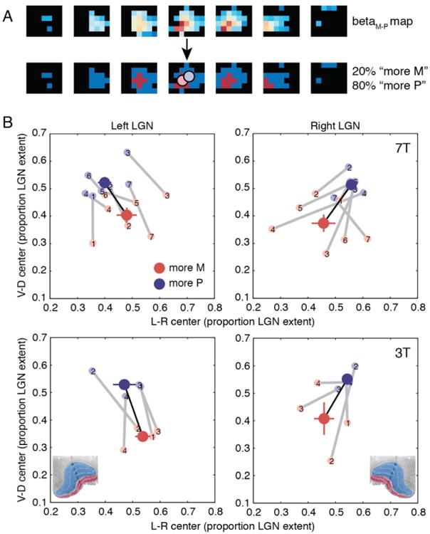
Spatial analysis of M-P maps. (A) Voxels were classified as “more M” or “more P” based on their beta_M-P values. The 20% of voxels with the largest beta_M-P values were assigned to the “more M” group, and the remaining 80% of voxels were assigned to the “more P” group, matching the volumetric proportions of the M and P subdivisions, as measured histologically. Spatial centers for the two groups, denoted by red and blue circles, are superimposed on the binarized map. An example right LGN (as in Figure 4) is shown. (B) Spatial centers of the M (red) and P (blue) voxel groups plotted for the medial-lateral and dorsal-ventral axes. Spatial centers were calculated in Talairach coordinates and are plotted as a proportion of the extent of each subject's LGN (based on the LGN localizer data from the same scanning session) along a given axis. Light circles connected by gray lines show M and P spatial centers for individual scanning sessions. Dark circles connected by black lines show the group mean, with error bars corresponding to the s.e.m. for each axis. Top: 7T. Bottom: 3T. Left: Left LGN. Right: Right LGN. Reference histological coronal sections of human LGN are included in the bottom plots (modified from Briggs and Usrey, 2011).

To test the reliability of these findings, we repeated the spatial centers analysis on a subset of approximately 50% of LGN voxels that had the best fits to the GLM (highest variance explained by the model). The mean separation between M group and P group centers along the dorsal-ventral axis was greater than that computed for all localized LGN voxels (7T: 1.06 mm vs. 0.77 mm, t(13) = 3.41, p = 0.0047; 3T: 1.54 mm vs. 1.07 mm, t(7) = 1.67, p = 0.14), and there was a high degree of consistency in spatial center layout across individual subjects and sessions (Figure 6). This increase in map quality following thresholding based on explained variance is what we would expect for the subset of voxels best driven by the M and P stimuli.

Figure 6.

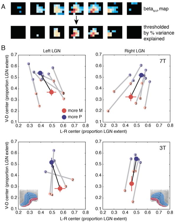
Spatial centers derived from the best-fit voxels. (A) Beta_M-P maps were thresholded according to the proportion of variance explained by the M/P GLM for each voxel's time series. Top: An example right LGN map (as in Figure 4). Bottom: The same map thresholded at 2% variance explained. (B) Spatial centers calculated as in Figure 5 for only those voxels with the highest proportions of variance explained (proportion > 2% for 7T and 0.4% for 3T, see Figure 7). These thresholds result in the inclusion of about half of all LGN ROI voxels across subjects. All other conventions as in Figure 5. Reference histological coronal sections of human LGN are included in the bottom plots (modified from Briggs and Usrey, 2011).

To ensure that the spatial center layout we observed did not depend on a particular choice of explained variance threshold, we calculated M and P group centers across a wide range of thresholds (Figure 7). The anatomically expected spatial arrangement of M and P group centers was consistently observed for both the dorsal-ventral and medial-lateral axes. Analysis of the anterior-posterior axis showed a tendency for the M group center to be more anterior than the P group center, but this did not reach significance at either field strength for the set of all localized LGN voxels and was less consistent across thresholds than the separations along the other two axes. Smaller separation along the anterior-posterior axis is expected from human LGN anatomy; both M and P layers are present throughout the anterior-posterior extent of the structure (Hickey and Guillery, 1979).

Figure 7.

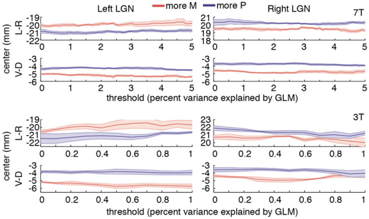
M-P map consistency across a range of LGN threshold values. Separation between spatial centers of “more M” group (red line) and “more P” group (blue line) along the medial-lateral and dorsal-ventral axes over a range of LGN threshold values. For a given threshold, an LGN voxel was included in the analysis if its proportion of variance explained by the GLM exceeded that threshold. Group data for all 7T (top) and 3T (bottom) sessions are shown in Talairach coordinates. Shaded regions show standard errors of the mean across sessions, after data points from each session were re-centered (via an additive shift) to the mean value across all sessions, voxel groups, and thresholds, in order to normalize for overall differences in LGN location across individual brains.

To evaluate the relative contributions of M and P responses to the M-P spatial gradient we observed, we repeated the spatial centers analysis on the M and P maps separately. For M responses, the 20% of voxels with the highest beta_M values were defined as the “more M” group and the other 80% were the “less M” group. For P responses, the 80% of voxels with the highest beta_P values comprised the “more P” group, and the other 20% were the “less P” group. We specifically considered the dorsal-ventral axis for this analysis, because this is the axis along which spatial separation of M and P voxels should be clearest based on anatomy (Hickey and Guillery, 1979). The ventrally-weighted gradient of beta_M-P values we observed is consistent with two alternatives for the individual M and P gradients (Figure 8A): 1) opposing gradients (ventrally-weighted M and dorsally-weighted P) or 2) aligned gradients with different gains (e.g., strong ventrally-weighted M and weak ventrally-weighted P). Such aligned gradients could arise, for example, from an underlying gradient in vascular density across the LGN. Our results provide evidence for two gradients in opposing directions, with both M and P maps having the dorsal-ventral orientation expected from LGN anatomy in 12/14 7T hemispheres and 4/8 3T hemispheres (chance = 25%, Figure 8B). Our consistent finding of opposing directions of M and P gradients shows that the M-P map gradients we have found (Figures 4-7) are not driven exclusively by either the M or P stimulus but rather reflect anatomically correct maps for both stimulus types. This correspondence between the type of visual stimulus presentation (M or P) and the orientation of the BOLD gradient makes alternative explanations for M-P gradients based on non-visual structures (such as nearby ventricles, surrounding tissue, or vasculature) very unlikely.

Figure 8.

Components of the M-P spatial gradient. (A) Two possible arrangements of beta_M and beta_P gradients (left) that could give rise to a spatial gradient in the beta_M-P map (right); only the dorsal-ventral axis is shown. (B) Separation of spatial centers along the dorsal-ventral axis in M maps (red bars) and P maps (blue bars) for the left and right LGN ROIs from each session. Separations between “more M” and “less M” centers from M maps and “more P” and “less P” centers from P maps (see Material and Methods) are plotted, in Talairach coordinates. Ventrally-weighted maps are shown as negative values, and dorsally-weighted maps are shown as positive values. Hemispheres with both ventrally-weighted M maps and dorsally-weighted P maps indicate two opposing gradients that are consistent with known anatomical organization. Top: 7T. Bottom: 3T.

Another test of the validity of our M/P localization procedure is consistency of M-P maps across experimental sessions. To quantify this consistency, we assessed individual subject M-P map reliability across scanning sessions on different days. We calculated the correlation of M-P values across voxels after the maps were projected onto a high-resolution anatomical volume and resampled to the resolution of that volume. We considered only the overlapping portion of the aligned LGN ROIs from the two sessions; the mean overlap (ROI intersection / ROI union) was 30% (SD 9%; range 13-44%). Some subjects were scanned multiple times at the same field strength (3T or 7T), and some were scanned at different field strengths. Significant positive cross-session correlations at the single-voxel level were observed in 6/6 same-field strength and 3/6 different-field strength comparisons, as assessed by randomization tests (all p < 0.005; Figure 9). The three comparisons that did not show positive correlations all involved a single session (Subject 2; 7T session 4) that had low overlap with the LGN ROIs from the comparison sessions (mean 18% overlap for this session vs. 34% for all other comparisons). This low overlap probably resulted from difficulty aligning functional images from 7T session 4 to the anatomical volume due to distortion and dropout in cortical regions that would ordinarily serve as landmarks for alignment.

Figure 9.

M-P map reliability across sessions. Correlations between LGN voxel beta_M-P values across scanning sessions from the same subject, after aligning and resampling the functional maps to that subject's anatomical space. Each bar shows the test-retest correlation for one hemisphere. Error bars are bootstrapped 95% confidence intervals. Labels indicate subject and session numbers for the two sessions being compared (see Table 1).

The mean cross-session correlation across all comparison hemispheres was 0.23 (range -0.18 to 0.51) and was significantly greater than zero at the group level (one-sample t-test of Fisher z-transformed correlation coefficients, t(11) = 3.78, p = 0.0031; Figure 9). Taken together, these results demonstrate that the M-P maps were reliable across sessions for individual subjects. Examples of low test-retest reliability seemed to reflect different positions of the entire LGN ROI when aligned to the anatomical images rather than differences in map organization, suggesting that, at least within the parameter space we used, test-retest reliability does not strongly depend on field strength or specific scanning parameters.

In addition to cross-session reliability, we calculated reliability measures between pairs of 5-minute runs and across blocks within single runs. First, we calculated the inter-run correlation of M-P maps generated from individual runs within a single scanning session. This measure indicates the map quality of a single run and is therefore a useful measure of SNR. Second, we computed functional SNR across blocks within single runs as the F-statistic of a one-way ANOVA of mean response amplitudes in M, P, and blank stimulus blocks. Inter-run correlations differed between field strengths, with higher mean correlations for 7T (0.43 +/- 0.04) than for 3T (0.16 +/- 0.03). Likewise, mean F-statistic values were higher at 7T (6.86 +/- 0.52) than at 3T (2.37 +/- 0.16). Thus, in our study, functional SNR was 2.5-3 times as high for 7T as for 3T scans, even though voxel volume was smaller at 7T (1.875-3.375 mm³) than at 3T (4.594 mm³).

Discussion

A critical step toward understanding the roles of the LGN in human vision in both health and disease is the ability to noninvasively measure functional signals from M and P subdivisions. This goal has proven elusive for two major reasons. The first is the challenge of measuring brain activity at the depth and spatial resolution required to segregate the M and P subdivisions within the LGN, a small brain structure that extends only 5-10 mm in any spatial dimension. The second has been the lack of a paradigm that differentially drives responses in LGN M and P subdivisions that can in turn be measured noninvasively. By using high-resolution fMRI to measure functional signals from the LGN combined with stimuli specially designed to differentially drive responses in M and P subdivisions, we found gradients of M and P voxel responses across human LGN with spatial organization in excellent agreement with known LGN anatomy. This is the first physiological evidence that the functional properties of human M and P subdivisions are similar to those of the monkey LGN.

In developing an fMRI M/P mapping paradigm guided by prior electrophysiological studies of M and P neurons, possible differences between electrophysiological and fMRI measurements from the LGN must be considered. One possible difference is the influence of neuronal feedback on the measured response. The BOLD signal likely reflects synaptic activity more than spiking output (Logothetis and Wandell, 2004). This, combined with the fact that the LGN receives about 90% of its input from sites other than the retina, including 30% from V1 (Sherman and Guillery, 2006; Van Horn et al., 2000), means that feedback projections are likely to significantly contribute to the BOLD response measured in the LGN. There is considerable evidence that feedback projections from V1 to LGN are M- and P-stream specific (Briggs and Usrey, 2009, 2011), but the functions of these projections and their possible influence on the BOLD signal is still not well understood. Our findings suggest that, even in the likely presence of feedback signals in the measured fMRI responses, the same stimuli that drive differential M and P neuron responses also evoke differential BOLD responses.

Previous studies have noninvasively measured activity in the human LGN using fMRI (Anderson et al., 2009; Chen and Zhu, 2001; Chen et al., 1999; D'Souza et al., 2011; Haynes et al., 2005; Kastner et al., 2004; Mullen et al., 2008; Mullen et al., 2010; O'Connor et al., 2002; Parkes et al., 2004; Schneider, 2011; Schneider and Kastner, 2009; Schneider et al., 2004; Uğurbil et al., 1999; Wunderlich et al., 2005), and there has been one attempt to localize the M and P subdivisions using fMRI (Schneider et al., 2004). In that study, stimulus contrast was manipulated (either 10% or 100% contrast-reversing checkerboard stimuli) to attempt to dissociate the M and P subdivisions. Voxels were classified as M if they responded similarly to the two contrast levels and P if they responded more to the high contrast checkerboard. This classification was based on the logic that M neuronal responses saturate at low contrasts, while P neuronal responses continue to increase across a greater contrast range in the macaque (Derrington and Lennie, 1984; Kaplan and Shapley, 1982). The resulting M and P classification maps were presented for two subjects. However, these maps do not appear to exhibit the 3D spatial organization expected from anatomy – perhaps because the manipulation of only a single stimulus dimension limited map quality – and no attempt was made to quantify the spatial organization of the maps or establish their consistency across subjects. We show here that simultaneous manipulation of multiple stimulus dimensions selected to differentially drive M and P layers provides a robust approach to M and P mapping with fMRI, in which the anatomically expected map organization could be observed and quantified in nearly every hemisphere we studied.

Although our localizer effectively and reliably generates M-P maps, the small size of the LGN relative to voxel size as well as variability across subjects leave at least two aspects of M/P localization that could be improved. First, the M-P maps we observed were more like gradients across the structure than bimodal maps with separate M and P peaks. The distribution of beta_M-P values in a given hemisphere was also typically unimodal. A likely contributor to this unimodality is partial voluming: single voxels that straddle the M/P border will contain both M and P neurons. Another possible contributor to the unimodality of response amplitude distributions is the mixing of M- and P-related BOLD signals in common vascular networks. To improve mapping and voxel classification, future studies may employ even higher spatial resolution to reduce partial volume effects. Spin-echo sequences at 7T or higher field strengths could also be used to minimize contributions of the macro-vasculature (Yacoub et al., 2003).

A second area for improvement is the classification of M and P voxels in a way that better accounts for individual differences. In our study, we defined M and P subdivisions according to a fixed 20/80 volumetric ratio of M and P layers. However, this ratio has been shown to vary across individuals (Andrews et al., 1997; Hickey and Guillery, 1979; Selemon and Begovic, 2007), adding uncertainty to the voxel classification, especially for those voxels with M-P values near the classification boundary. This means that, in its current form, the classification method we have employed is not suitable for measuring the absolute volumes of the M and P subdivisions. In the future, more sophisticated voxel classification approaches combining functional and anatomical information could generate more accurate classification boundaries. For functional studies, both partial volume effects and classification limitations can be overcome to some extent by selecting only the most M-like and P-like voxels for subsequent analyses, based on the distribution of M-P values that are calculated for each voxel.

Our results suggest that both 7T and 3T field strengths can provide sufficient signal and spatial resolution for consistent M/P mapping of human LGN. We also found advantages of 7T over 3T, including: higher functional SNR; more variance explained by the GLM; higher reliability across runs; and more consistent dorsal-ventral gradients in both M and P maps across hemispheres. As all these advantages were evident for 7T voxel sizes that were similar to or smaller than the 3T voxel sizes used, they likely arise from a combination of higher MR signal at 7T and reduced partial volume effects at smaller voxel sizes. The higher SNR and reliability across runs at 7T also enable M/P localization using fewer runs compared to 3T. Therefore, researchers seeking to localize the M and P subdivisions and then conduct other experimental tasks investigating the functions of the subdivisions would benefit from the use of 7T.

The ability to noninvasively map the M and P subdivisions of human LGN presents opportunities to study the roles of these subdivisions in normal human vision as well as in clinical disorders. Since fMRI is an excellent tool for the study of large-scale brain networks, M/P mapping of the LGN enables functional investigations of parallel thalamocortical processing pathways. Modulations of LGN activity have also been observed during selective visual attention (McAlonan et al., 2008; O'Connor et al., 2002; Schneider, 2011; Schneider and Kastner, 2009; Vanduffel et al., 2000) and perceptual fluctuations during binocular rivalry (Haynes et al., 2005; Wunderlich et al., 2005), supporting the idea that the human LGN may support higher-level aspects of vision, as opposed to operating as a simple sensory relay (Kastner et al., 2006). Indeed, reciprocal interactions between cortex and thalamus are increasingly recognized as central to sensory system function (Briggs and Usrey, 2008; Sherman and Guillery, 2002). The differential roles of the M and P subdivisions in such higher-level visual functions are currently not well understood, but behavioral studies suggest different contributions from the two pathways to spatial attention (Cheng et al., 2004; Theeuwes, 1995; Yeshurun, 2004; Yeshurun and Levy, 2003; Yeshurun and Sabo, 2012) and perceptual selection (Denison and Silver, 2012). Measuring human M and P responses with fMRI during a variety of behavioral tasks is an exciting direction for future work.

Functional studies of the M and P subdivisions in healthy individuals and patient populations may additionally further our understanding of human disorders. In particular, dysfunction of the M system has been implicated in dyslexia (Demb et al., 1998a; Demb et al., 1998b; Kubová et al., 1996; Lehmkuhle et al., 1993; Livingstone et al., 1991; Stein and Walsh, 1997) and schizophrenia (Butler and Javitt, 2005; Kandil et al., 2013; Núñez et al., 2013), but clear physiological tests of the hypothesized links between M stream abnormalities and specific diseases have not yet materialized. Stream-specific abnormalities have also been associated with albinism (Guillery et al., 1975) and degenerative disorders including multiple sclerosis, Parkinson's disease, and Alzheimer's disease (Yoonessi and Yoonessi, 2011). Better understanding of the relationship between stream-specific abnormalities and disease state offers the potential for simple visual tests that could aid diagnosis of these disorders.

In conclusion, we have demonstrated that the combination of high spatial resolution fMRI and optimized stimuli enables reliable functional mapping of the M and P subdivisions of human LGN, advancing the noninvasive study of parallel processing pathways in the human visual system.

Highlights.

• Functional mapping of the M and P subdivisions of human LGN with 7T and 3T fMRI

• Stimuli based on electrophysiology in non-human primates allow human LGN mapping

• Spatial organization of M-like and P-like voxels consistent with known LGN anatomy

• Reliable M/P maps across test-retest sessions for individual subjects

References

- Anderson EJ, Dakin SC, Rees G. Monocular signals in human lateral geniculate nucleus reflect the Craik-Cornsweet-O'Brien effect. Journal of Vision. 2009;9:14 11–18. doi: 10.1167/9.12.14. [DOI] [PubMed] [Google Scholar]
- Andrews TJ, Halpern SD, Purves D. Correlated size variations in human visual cortex, lateral geniculate nucleus, and optic tract. Journal of Neuroscience. 1997;17:2859–2868. doi: 10.1523/JNEUROSCI.17-08-02859.1997. [DOI] [PMC free article] [PubMed] [Google Scholar]
- Boynton GM, Engel SA, Glover GH, Heeger DJ. Linear systems analysis of functional magnetic resonance imaging in human V1. J Neurosci. 1996;16:4207–4221. doi: 10.1523/JNEUROSCI.16-13-04207.1996. [DOI] [PMC free article] [PubMed] [Google Scholar]
- Brainard DH. The Psychophysics Toolbox. Spat Vis. 1997;10:433–436. [PubMed] [Google Scholar]
- Briggs F, Usrey WM. Emerging views of corticothalamic function. Current Opinion in Neurobiology. 2008;18:403–407. doi: 10.1016/j.conb.2008.09.002. [DOI] [PMC free article] [PubMed] [Google Scholar]
- Briggs F, Usrey WM. Parallel processing in the corticogeniculate pathway of the macaque monkey. Neuron. 2009;62:135–146. doi: 10.1016/j.neuron.2009.02.024. [DOI] [PMC free article] [PubMed] [Google Scholar]
- Briggs F, Usrey WM. Corticogeniculate feedback and parallel processing in the primate. The Journal of Physiology. 2011;589:33–40. doi: 10.1113/jphysiol.2010.193599. [DOI] [PMC free article] [PubMed] [Google Scholar]
- Butler PD, Javitt DC. Early-stage visual processing deficits in schizophrenia. Current Opinion in Psychiatry. 2005;18:151–157. doi: 10.1097/00001504-200503000-00008. [DOI] [PMC free article] [PubMed] [Google Scholar]
- Chen W, Zhu XH. Correlation of activation sizes between lateral geniculate nucleus and primary visual cortex in humans. Magnetic Resonance in Medicine. 2001;45:202–205. doi: 10.1002/1522-2594(200102)45:2<202::aid-mrm1027>3.0.co;2-s. [DOI] [PubMed] [Google Scholar]
- Chen W, Zhu XH, Thulborn KR, Uğurbil K. Retinotopic mapping of lateral geniculate nucleus in humans using functional magnetic resonance imaging. Proceedings of the National Academy of Sciences, USA. 1999;96:2430–2434. doi: 10.1073/pnas.96.5.2430. [DOI] [PMC free article] [PubMed] [Google Scholar]
- Cheng A, Eysel UT, Vidyasagar TR. The role of the magnocellular pathway in serial deployment of visual attention. Eur J Neurosci. 2004;20:2188–2192. doi: 10.1111/j.1460-9568.2004.03675.x. [DOI] [PubMed] [Google Scholar]
- D'Souza DV, Auer T, Strasburger H, Frahm J, Lee BB. Temporal frequency and chromatic processing in humans: An fMRI study of the cortical visual areas. Journal of Vision. 2011;11:8–8. doi: 10.1167/11.8.8. [DOI] [PubMed] [Google Scholar]
- de Courten C, Garey LJ. Morphology of the neurons in the human lateral geniculate nucleus and their normal development. A Golgi study. Experimental Brain Research. 1982;47:159–171. doi: 10.1007/BF00239375. [DOI] [PubMed] [Google Scholar]
- De Valois K, De Valois RL. Color Vision. In: De Valois K, editor. Seeing. Academic Press; San Diego, CA: 2000. pp. 129–176. [Google Scholar]
- De Valois RL, Morgan H, Snodderly DM. Psychophysical studies of monkey vision. 3. Spatial luminance contrast sensitivity tests of macaque and human observers. Vision Research. 1974a;14:75–81. doi: 10.1016/0042-6989(74)90118-7. [DOI] [PubMed] [Google Scholar]
- De Valois RL, Morgan HC, Polson MC, Mead WR, Hull EM. Psychophysical studies of monkey vision. I. Macaque luminosity and color vision tests. Vision Research. 1974b;14:53–67. doi: 10.1016/0042-6989(74)90116-3. [DOI] [PubMed] [Google Scholar]
- Demb JB, Boynton GM, Best M, Heeger DJ. Psychophysical evidence for a magnocellular pathway deficit in dyslexia. Vision Research. 1998a;38:1555–1559. doi: 10.1016/s0042-6989(98)00075-3. [DOI] [PubMed] [Google Scholar]
- Demb JB, Boynton GM, Heeger DJ. Functional magnetic resonance imaging of early visual pathways in dyslexia. Journal of Neuroscience. 1998b;18:6939–6951. doi: 10.1523/JNEUROSCI.18-17-06939.1998. [DOI] [PMC free article] [PubMed] [Google Scholar]
- Denison RN, Silver MA. Distinct contributions of the magnocellular and parvocellular visual streams to perceptual selection. Journal of Cognitive Neuroscience. 2012;24:246–259. doi: 10.1162/jocn_a_00121. [DOI] [PMC free article] [PubMed] [Google Scholar]
- Derrington AM, Lennie P. Spatial and temporal contrast sensitivities of neurones in lateral geniculate nucleus of macaque. The Journal of Physiology. 1984;357:219–240. doi: 10.1113/jphysiol.1984.sp015498. [DOI] [PMC free article] [PubMed] [Google Scholar]
- Feinberg DA, Moeller S, Smith SM, Auerbach E, Ramanna S, Gunther M, Glasser MF, Miller KL, Ugurbil K, Yacoub E. Multiplexed echo planar imaging for sub-second whole brain FMRI and fast diffusion imaging. PLoS ONE. 2010;5:e15710. doi: 10.1371/journal.pone.0015710. [DOI] [PMC free article] [PubMed] [Google Scholar]
- Guillery RW, Okoro AN, Witkop CJ. Abnormal visual pathways in the brain of a human albino. Brain Research. 1975;96:373–377. doi: 10.1016/0006-8993(75)90750-7. [DOI] [PubMed] [Google Scholar]
- Haynes JD, Deichmann R, Rees G. Eye-specific effects of binocular rivalry in the human lateral geniculate nucleus. Nature. 2005;438:496–499. doi: 10.1038/nature04169. [DOI] [PMC free article] [PubMed] [Google Scholar]
- Hickey TL, Guillery RW. Variability of laminar patterns in the human lateral geniculate nucleus. Journal of Comparative Neurology. 1979;183:221–246. doi: 10.1002/cne.901830202. [DOI] [PubMed] [Google Scholar]
- Hicks TP, Lee BB, Vidyasagar TR. The responses of cells in macaque lateral geniculate nucleus to sinusoidal gratings. The Journal of Physiology. 1983;337:183–200. doi: 10.1113/jphysiol.1983.sp014619. [DOI] [PMC free article] [PubMed] [Google Scholar]
- Hubel DH, Livingstone MS. Color and contrast sensitivity in the lateral geniculate body and primary visual cortex of the macaque monkey. Journal of Neuroscience. 1990;10:2223–2237. doi: 10.1523/JNEUROSCI.10-07-02223.1990. [DOI] [PMC free article] [PubMed] [Google Scholar]
- Jenkinson M, Bannister P, Brady M, Smith S. Improved optimization for the robust and accurate linear registration and motion correction of brain images. NeuroImage. 2002;17:825–841. doi: 10.1016/s1053-8119(02)91132-8. [DOI] [PubMed] [Google Scholar]
- Kandil FI, Pedersen A, Wehnes J, Ohrmann P. High-level, but not low-level, motion perception is impaired in patients with schizophrenia. Neuropsychology. 2013;27:60–68. doi: 10.1037/a0031300. [DOI] [PubMed] [Google Scholar]
- Kaplan E, Shapley RM. X and Y cells in the lateral geniculate nucleus of macaque monkeys. The Journal of Physiology. 1982;330:125–143. doi: 10.1113/jphysiol.1982.sp014333. [DOI] [PMC free article] [PubMed] [Google Scholar]
- Kastner S, O'Connor DH, Fukui MM, Fehd HM, Herwig U, Pinsk MA. Functional imaging of the human lateral geniculate nucleus and pulvinar. Journal of Neurophysiology. 2004;91:438–448. doi: 10.1152/jn.00553.2003. [DOI] [PubMed] [Google Scholar]
- Kastner S, Schneider KA, Wunderlich K. Beyond a relay nucleus: neuroimaging views on the human LGN. Progress in Brain Research. 2006;155:125–143. doi: 10.1016/S0079-6123(06)55008-3. [DOI] [PubMed] [Google Scholar]
- Kleinschmidt A, Lee BB, Requardt M, Frahm J. Functional mapping of color processing by magnetic resonance imaging of responses to selective P- and M-pathway stimulation. Exp Brain Res. 1996;110:279–288. doi: 10.1007/BF00228558. [DOI] [PubMed] [Google Scholar]
- Kubová Z, Kuba M, Peregrin J, Nováková V. Visual evoked potential evidence for magnocellular system deficit in dyslexia. Physiological Research. 1996;45:87–89. [PubMed] [Google Scholar]
- Lehmkuhle S, Garzia RP, Turner L, Hash T, Baro JA. A defective visual pathway in children with reading disability. New England Journal of Medicine. 1993;328:989–996. doi: 10.1056/NEJM199304083281402. [DOI] [PubMed] [Google Scholar]
- Liu CSJ, Bryan RN, Miki A, Woo JH, Liu GT, Elliott MA. Magnocellular and parvocellular visual pathways have different blood oxygen level-dependent signal time courses in human primary visual cortex. American Journal of Neuroradiology. 2006;27:1628–1634. [PMC free article] [PubMed] [Google Scholar]
- Livingstone M, Hubel D. Segregation of form, color, movement, and depth: anatomy, physiology, and perception. Science. 1988;240:740–749. doi: 10.1126/science.3283936. [DOI] [PubMed] [Google Scholar]
- Livingstone MS, Hubel DH. Psychophysical evidence for separate channels for the perception of form, color, movement, and depth. Journal of Neuroscience. 1987;7:3416–3468. doi: 10.1523/JNEUROSCI.07-11-03416.1987. [DOI] [PMC free article] [PubMed] [Google Scholar]
- Livingstone MS, Rosen GD, Drislane FW, Galaburda AM. Physiological and anatomical evidence for a magnocellular defect in developmental dyslexia. Proceedings of the National Academy of Sciences, USA. 1991;88:7943–7947. doi: 10.1073/pnas.88.18.7943. [DOI] [PMC free article] [PubMed] [Google Scholar]
- Logothetis NK, Wandell BA. Interpreting the BOLD signal. Annual Review of Physiology. 2004;66:735–769. doi: 10.1146/annurev.physiol.66.082602.092845. [DOI] [PubMed] [Google Scholar]
- Maunsell JH, Ghose GM, Assad JA, McAdams CJ, Boudreau CE, Noerager BD. Visual response latencies of magnocellular and parvocellular LGN neurons in macaque monkeys. Visual Neuroscience. 1999;16:1–14. doi: 10.1017/s0952523899156177. [DOI] [PubMed] [Google Scholar]
- McAlonan K, Cavanaugh J, Wurtz RH. Guarding the gateway to cortex with attention in visual thalamus. Nature. 2008;456:391–394. doi: 10.1038/nature07382. [DOI] [PMC free article] [PubMed] [Google Scholar]
- Merigan WH. Chromatic and achromatic vision of macaques: role of the P pathway. Journal of Neuroscience. 1989;9:776–783. doi: 10.1523/JNEUROSCI.09-03-00776.1989. [DOI] [PMC free article] [PubMed] [Google Scholar]
- Moeller S, Yacoub E, Olman CA, Auerbach E, Strupp J, Harel N, Ugurbil K. Multiband multislice GE-EPI at 7 tesla, with 16-fold acceleration using partial parallel imaging with application to high spatial and temporal whole-brain fMRI. Magnetic Resonance in Medicine. 2010;63:1144–1153. doi: 10.1002/mrm.22361. [DOI] [PMC free article] [PubMed] [Google Scholar]
- Mullen KT, Dumoulin SO, Hess RF. Color responses of the human lateral geniculate nucleus: selective amplification of S-cone signals between the lateral geniculate nucleon and primary visual cortex measured with high-field fMRI. European Journal of Neuroscience. 2008;28:1911–1923. doi: 10.1111/j.1460-9568.2008.06476.x. [DOI] [PMC free article] [PubMed] [Google Scholar]
- Mullen KT, Thompson B, Hess RF. Responses of the human visual cortex and LGN to achromatic and chromatic temporal modulations: an fMRI study. Journal of Vision. 2010;10:13. doi: 10.1167/10.13.13. [DOI] [PubMed] [Google Scholar]
- Nassi JJ, Callaway EM. Parallel processing strategies of the primate visual system. Nature Reviews: Neuroscience. 2009;10:360–372. doi: 10.1038/nrn2619. [DOI] [PMC free article] [PubMed] [Google Scholar]
- Nestares O, Heeger DJ. Robust multiresolution alignment of MRI brain volumes. Magn Reson Med. 2000;43:705–715. doi: 10.1002/(sici)1522-2594(200005)43:5<705::aid-mrm13>3.0.co;2-r. [DOI] [PubMed] [Google Scholar]
- Núñez D, Rauch J, Herwig K, Rupp A, Andermann M, Weisbrod M, Resch F, Oelkers-Ax R. Evidence for a magnocellular disadvantage in early-onset schizophrenic patients: A source analysis of the N80 visual-evoked component. Schizophrenia Research. 2013 doi: 10.1016/j.schres.2012.12.007. [DOI] [PubMed] [Google Scholar]
- O'Connor DH, Fukui MM, Pinsk MA, Kastner S. Attention modulates responses in the human lateral geniculate nucleus. Nature Neuroscience. 2002;5:1203–1209. doi: 10.1038/nn957. [DOI] [PubMed] [Google Scholar]
- Parkes LM, Fries P, Kerskens CM, Norris DG. Reduced BOLD response to periodic visual stimulation. NeuroImage. 2004;21:236–243. doi: 10.1016/j.neuroimage.2003.08.025. [DOI] [PubMed] [Google Scholar]
- Pelli DG. The VideoToolbox software for visual psychophysics: transforming numbers into movies. Spat Vis. 1997;10:437–442. [PubMed] [Google Scholar]
- Power JD, Barnes KA, Snyder AZ, Schlaggar BL, Petersen SE. Spurious but systematic correlations in functional connectivity MRI networks arise from subject motion. NeuroImage. 2012;59:2142–2154. doi: 10.1016/j.neuroimage.2011.10.018. [DOI] [PMC free article] [PubMed] [Google Scholar]
- Reid RC, Shapley RM. Space and time maps of cone photoreceptor signals in macaque lateral geniculate nucleus. Journal of Neuroscience. 2002;22:6158–6175. doi: 10.1523/JNEUROSCI.22-14-06158.2002. [DOI] [PMC free article] [PubMed] [Google Scholar]
- Schiller PH, Logothetis NK, Charles ER. Functions of the colour-opponent and broad-band channels of the visual system. Nature. 1990;343:68–70. doi: 10.1038/343068a0. [DOI] [PubMed] [Google Scholar]
- Schiller PH, Malpeli JG. Functional specificity of lateral geniculate nucleus laminae of the rhesus monkey. Journal of Neurophysiology. 1978;41:788–797. doi: 10.1152/jn.1978.41.3.788. [DOI] [PubMed] [Google Scholar]
- Schneider KA. Subcortical mechanisms of feature-based attention. Journal of Neuroscience. 2011;31:8643–8653. doi: 10.1523/JNEUROSCI.6274-10.2011. [DOI] [PMC free article] [PubMed] [Google Scholar]
- Schneider KA, Kastner S. Effects of sustained spatial attention in the human lateral geniculate nucleus and superior colliculus. Journal of Neuroscience. 2009;29:1784–1795. doi: 10.1523/JNEUROSCI.4452-08.2009. [DOI] [PMC free article] [PubMed] [Google Scholar]
- Schneider KA, Richter MC, Kastner S. Retinotopic organization and functional subdivisions of the human lateral geniculate nucleus: a high-resolution functional magnetic resonance imaging study. Journal of Neuroscience. 2004;24:8975–8985. doi: 10.1523/JNEUROSCI.2413-04.2004. [DOI] [PMC free article] [PubMed] [Google Scholar]
- Selemon LD, Begovic A. Stereologic analysis of the lateral geniculate nucleus of the thalamus in normal and schizophrenic subjects. Psychiatry Research. 2007;151:1–10. doi: 10.1016/j.psychres.2006.11.003. [DOI] [PMC free article] [PubMed] [Google Scholar]
- Setsompop K, Gagoski BA, Polimeni JR, Witzel T, Wedeen VJ, Wald LL. Blipped-controlled aliasing in parallel imaging for simultaneous multislice echo planar imaging with reduced g-factor penalty. Magnetic Resonance in Medicine. 2012;67:1210–1224. doi: 10.1002/mrm.23097. [DOI] [PMC free article] [PubMed] [Google Scholar]
- Shapley R. Visual sensitivity and parallel retinocortical channels. Annual Review of Psychology. 1990;41:635–658. doi: 10.1146/annurev.ps.41.020190.003223. [DOI] [PubMed] [Google Scholar]
- Sherman SM, Guillery RW. The role of the thalamus in the flow of information to the cortex. Philosophical Transactions of the Royal Society of London, Series B: Biological Sciences. 2002;357:1695–1708. doi: 10.1098/rstb.2002.1161. [DOI] [PMC free article] [PubMed] [Google Scholar]
- Sherman SM, Guillery RW. Exploring the Thalamus and Its Role in Cortical Function. The MIT Press; Cambridge, MA: 2006. [Google Scholar]
- Smith AM, Lewis BK, Ruttimann UE, Ye FQ, Sinnwell TM, Yang Y, Duyn JH, Frank JA. Investigation of low frequency drift in fMRI signal. NeuroImage. 1999;9:526–533. doi: 10.1006/nimg.1999.0435. [DOI] [PubMed] [Google Scholar]
- Stein J, Walsh V. To see but not to read; the magnocellular theory of dyslexia. Trends in Neurosciences. 1997 doi: 10.1016/s0166-2236(96)01005-3. [DOI] [PubMed] [Google Scholar]
- Straw AD. Vision egg: an open-source library for realtime visual stimulus generation. Front Neuroinform. 2008;2:4. doi: 10.3389/neuro.11.004.2008. [DOI] [PMC free article] [PubMed] [Google Scholar]
- Theeuwes J. Abrupt luminance change pops out; abrupt color change does not. Percept Psychophys. 1995;57:637–644. doi: 10.3758/bf03213269. [DOI] [PubMed] [Google Scholar]
- Uğurbil K, Hu X, Chen W, Zhu XH, Kim SG, Georgopoulos A. Functional mapping in the human brain using high magnetic fields. Philosophical Transactions of the Royal Society of London, Series B: Biological Sciences. 1999;354:1195–1213. doi: 10.1098/rstb.1999.0474. [DOI] [PMC free article] [PubMed] [Google Scholar]
- Van Horn SC, Erişir A, Sherman SM. Relative distribution of synapses in the A-laminae of the lateral geniculate nucleus of the cat. Journal of Comparative Neurology. 2000;416:509–520. [PubMed] [Google Scholar]
- Vanduffel W, Tootell RB, Orban GA. Attention-dependent suppression of metabolic activity in the early stages of the macaque visual system. Cerebral Cortex. 2000;10:109–126. doi: 10.1093/cercor/10.2.109. [DOI] [PubMed] [Google Scholar]
- Wunderlich K, Schneider KA, Kastner S. Neural correlates of binocular rivalry in the human lateral geniculate nucleus. Nature Neuroscience. 2005;8:1595–1602. doi: 10.1038/nn1554. [DOI] [PMC free article] [PubMed] [Google Scholar]
- Yacoub E, Duong TQ, Van De Moortele PF, Lindquist M, Adriany G, Kim SG, Ugurbil K, Hu X. Spin-echo fMRI in humans using high spatial resolutions and high magnetic fields. Magn Reson Med. 2003;49:655–664. doi: 10.1002/mrm.10433. [DOI] [PubMed] [Google Scholar]
- Yeshurun Y. Isoluminant stimuli and red background attenuate the effects of transient spatial attention on temporal resolution. Vision Research. 2004;44:1375–1387. doi: 10.1016/j.visres.2003.12.016. [DOI] [PubMed] [Google Scholar]
- Yeshurun Y, Levy L. Transient spatial attention degrades temporal resolution. Psychological Science. 2003;14:225–231. doi: 10.1111/1467-9280.02436. [DOI] [PubMed] [Google Scholar]
- Yeshurun Y, Sabo G. Differential effects of transient attention on inferred parvocellular and magnocellular processing. Vision Research. 2012;74:21–29. doi: 10.1016/j.visres.2012.06.006. [DOI] [PubMed] [Google Scholar]
- Yoonessi A, Yoonessi A. Functional assessment of magno, parvo and konio-cellular pathways; current state and future clinical applications. Journal of Opthalmic & Vision Research. 2011;6:119–126. [PMC free article] [PubMed] [Google Scholar]
- Zarahn E, Aguirre GK, D'esposito M. Empirical analyses of BOLD fMRI statistics. I. Spatially unsmoothed data collected under null-hypothesis conditions. NeuroImage. 1997;5:179–197. doi: 10.1006/nimg.1997.0263. [DOI] [PubMed] [Google Scholar]
Associated Data
This section collects any data citations, data availability statements, or supplementary materials included in this article.