Robust Selection-based Sparse Shape Model for Lung Cancer Image Segmentation

Abstract

Accurate cellular level segmentation of lung cancer is the prerequisite to extract objective morphological features in digitized pathology specimens. It is of great importance for image-guided diagnosis and prognosis. However, it is challenging to correctly and robustly segment cells in lung cancer images due to cell occlusion or touching, intracellular inhomogeneity, background clutter, etc. In this paper, we present a novel segmentation algorithm combining a robust selection-based sparse shape model (top-down) and an efficient local repulsive balloon snake deformable model (bottom-up) to tackle these challenges. The algorithm has been extensively tested on 62 cases with over 6000 tumor cells. We experimentally demonstrate that the proposed algorithm can produce better performance than other state-of-the-art methods.

1 Introduction

Efficient and accurate cell segmentation on pathology images for lung cancer can provide diagnosis and prognosis support for improved characterization and personalized treatment, but it remains as a challenging problem due to cell occlusion/touching, densely clustering, size variation, intracellular inhomogeneity, etc. Segmentation methods that only rely on bottom-up information may not be sufficient to handle images exhibiting large inhomogeneities like lung cancer. Supervised learning [11], multi-reference level set [4], hierarchical partial matching [17], and various shape prior models [7,3,8,16,14] were proposed to address these challenges and achieved excellent performance. Recently, Zhang et al. [19] modeled shape prior using a sparse shape composition, which produces accurate organ-level segmentation in lung and liver images. Compared with the traditional PCA-based active shape model [7], sparse representation-based shape model can preserve local details [19].

Sparse shape model using all training shapes as the dictionary is inefficient for a large dataset. KSVD [1] is a popular dictionary learning algorithm which is also used in [19], however it is not designed as a discriminative and selection-based dictionary learning method with respect to classification and segmentation. In this work, we propose a novel and robust selection-based dictionary learning algorithm for cellular level shape modeling for lung cancer tumor cells. Different from KSVD, this method directly selects the most representative cellular shapes from the training dataset as dictionary bases. The robustness of the dictionary learning method is achieved by minimizing an integrated square error with a sparse constraint. In addition, an efficient online dictionary update scheme is designed to adaptively update dictionary bases. Finally, a novel local repulsive balloon snake is presented to fast deform shapes considering the requirement for touching cell segmentation.

2 Methodology

Figure 1 shows the framework of the whole segmentation algorithm. In the training stage, a cell boundary detector is learned using the method in [18]. The training cell shapes, after alignment with Procrustes analysis [7], are utilized to train a compact dictionary using the proposed selection-based dictionary learning method. In the testing stage, the seeds of the cells are automatically detected using a voting-based seed detection algorithm presented in [12], and these detected local minima (seeds) are used to initiate an adaptive H-minima transformation to obtain the initial shapes [5], one per cell. The algorithm alternately performs shape deformation using an efficient local repulsive balloon snake, and shape inference using the shape prior derived from the sparse shape model.

Fig. 1.

The flow chart of the proposed algorithm.

Robust Selection-based Sparse Shape Model

In this paper, cell shape v ∈ R^2m is represented by the concatenated 2D coordinates of m landmarks which are automatically detected by the rules: 1) The two endpoints of the major axis of the shape are selected as major landmarks. 2) All the other landmarks are interpolated along the shape. Given N cell shapes {v_i} aligned by Procrustes analysis [7], sparsity-based shape modeling aims to find a compact shape dictionary B = [b₁ b₂, ... b_K] ({b_k ∈ R^2m} are bases) and a sparse coefficient α such that any aligned shape v can be represented with a few bases: v = Bα+ε, where ε is the residual. Calculating α is called sparse coding, while dictionary learning can be formulated as

$$\underset{B,\left\{{\alpha }_i\right\}}{\min }\sum _{i=1}^N{\Vert v_i-B{\alpha }_i\Vert }_2+\lambda {\Vert {\alpha }_i\Vert }_1,$$ (1)

For a large cell shape dataset, it is intuitive to select a subset of the data as a shape repository that can sufficiently represent the whole dataset. This summarization can help remove outliers that are not the true representatives of the dataset and reduce the computational time for runtime optimization due to the decreased object-space dimension. Based on these considerations, we propose a novel selection-based dictionary learning method for sparse representation by minimizing a locality-constrained integrated squared error (ISE):

$$\underset{\theta }{\min }J\left(\theta \right)=\underset{\theta }{\min }[(\int g{(∊\mid \theta )}^{2}d∊-\frac{2}{N}\sum _{i=1}^{N}g({∊}_i\mid \theta ))+\lambda \sum _{i=1}^N\sum _{k=1}^M\mid {\alpha }_{ik}\mid {\Vert v_i-b_k\Vert }^2],s.t.1^T{\alpha }_i=1,\forall i,$$ (2)

where ε_i = v_i – Bα_i and α_i = [α_i1 α_i2 ... α_iK]^T · g(x|θ) is a parametric model with parameter θ. The first two terms forms the integrated squared error, which is robust to outliers [13]. The last term constrains local representation of bases with weighted sparse codes, and is used to encourage each cell to be sufficiently represented by its neighboring dictionary bases for similarity preserving, which is essential in the sparse reconstruction. The constraint 1^Tα_i = 1, $\forall i$ ensures the shift-invariance. The residual is modeled with multivariate normal distribution: ε_i ~ N(0, σ²I_2m). In this way g(ε_i|θ) = ξϕ(ε_i|0, σ²I_2m), where ξ denotes the percentage of the inlier shapes that need to be estimated and ϕ is the probability density function of multivariate normal distribution. Based on (2), the dictionary B and sparse coefficients {α_i} can be calculated by estimating θ = {ξ, B, α₁, α₂, .., α_N, σ²}.

Equation (2) can be solved by performing dictionary basis selection and sparse coding alternatively. As J(θ) in (2) is differentiable, projection based-gradient descent is utilized for minimization. We update the bases {b_k} by directly selecting shapes within each iteration. For sparse coding, we keep the dictionary fixed. Based on the sparse reconstruction criterion, the sparse coding objective function can be rewritten as:

$$\underset{\left\{{\alpha }_i\right\}i\in A}{\min }[\sum _{i\in A}{\Vert v_i-B{\alpha }_i\Vert }^2+\lambda \sum _{k=1}^K\mid {\alpha }_{ik}\mid {\Vert v_i-b_k\Vert }^2],s.t.1^T{\alpha }_i=1,i\in A,$$ (3)

where A is the set of indices corresponding to estimated inlier shapes. Locality-constrained linear coding (LLC) [15] is applied to (3) for sparse coding, where the neighboring bases are defined in terms of the Euclidean distances between the shape and dictionary bases.

Let B⁰ be the initial dictionary where the bases are randomly selected from the dataset, LLC is used in (3) to compute the current coefficients {α_i}. Meanwhile, the active set A is updated with the indices corresponding to the N · ξ shapes with the smallest reconstruction errors ${\Vert {∊}_i\Vert }_2^2$ in each iteration. At the t-th step, ${\theta }^t=\{{\xi }^t,B^t,{\alpha }_1^t,{\alpha }_2^t,\dots ,{\alpha }_N^t,{\sigma }^{t^2}\}$, and $B^t=[b_1^t,b_2^t,\dots ,b_K^t]$, denote the gradient of J(θ) in (2): $\frac{\partial J\left(\theta \right)}{\partial b_k}$, $\frac{\partial J\left(\theta \right)}{\partial {\sigma }^2}$, and $\frac{\partial J\left(\theta \right)}{\partial \xi }$, as J_bk, J_σ² and J_ξ, respectively. The basis b_k is updated by selecting the shape v_l which has the largest correlation between the displacement and the current $b_k^t$:

$$COR(x_l,b_k^t,J_{b_k})=\frac{{(v_l-b_k^t)}^T(-J_{b_k})}{{\Vert (v_l-b_k^t)\Vert }_2{\Vert -J_{b_k}\Vert }_2},$$ (4)

Let A^t represent a set of indices corresponding to the current estimated inliers, the current reconstruction error E^t and the ISE error F^t are defined as

$$E^t=\frac{{\sum }_{i=1,i\in A^t}^N{\Vert {∊}_i^t\Vert }_2^2}{{\sum }_{i=1}^{N}I(i\in A^t)},F^t={\xi }^{t^2}\varphi (0\mid 0,2{\sigma }^{t^2}{I}_{2m})-\frac{2{\xi }^t}{N}\sum _{i=1}^N\varphi ({∊}_i^t\mid 0,{\sigma }^{t^2}{I}_{2m}),$$ (5)

where I(x) is the indicator function. Assume that $E_{min}^t$ is the current reconstruction error, $E_{rep}^t$ is the reconstruction error after replacing the k-th basis with v_l, $F_{min}^t$ is the current ISE error, and $F_t^{rep}$ is the ISE error after replacing the k-th basis with v_l, then the replacement will be performed only if $E_{min}^t>E_{rep}^t$ and $F_{min}^t>F_{rep}^t$. The σ² and ξ are updated in the negative gradient directions:

$${\left({\sigma }^{t+1}\right)}^2={\sigma }^{t^2}-\Delta h_{{\sigma }^2}\cdot J_{{\sigma }^2},{\xi }^{t+1}={\xi }^t-\Delta h_{\xi }\cdot J_{\xi },$$ (6)

where Δh_σ² and Δh_ξ represent the learning rates.

Sparse Shape Model Update

Our algorithm supports efficient dictionary update. Recall that each basis b_k corresponds to one row α^(k) of the sparse coefficient matrix, and one basis is significant if it is used to represent many shapes in the sparse reconstruction such that α^(k) will have many nonzero elements with relatively large values. Therefore, we define the significance of basis b_k as

$$sig\left(b_k\right)=C\sum _{i=1}^N{\alpha }_i^{\left(k\right)}{e}^{\frac{-{\Vert {∊}_i\Vert }_2^2}{{\sigma }^2}},$$ (7)

where C denotes the normalized constant, and ${\alpha }_i^{\left(k\right)}$ is the i-th element of α^(k) which is the k-th row of the sparse coefficient matrix G = [α^(1)T α^(2)T ...α^(K)T]^T. The learned shape dictionary can be only updated when the current reconstruction error in (5) is larger than a threshold by replacing the current least significant basis with the most important one generated from the new images. This represents the case that cell shapes change dramatically.

Shape Deformation

For shape deformation, we propose a novel repulsive balloon snake (RBS) with locality constraint. We introduce a local repulsive term into the model in [6] to handle touching cells so that each point on the i-th shape v_i will be driven by both its own internal/external forces, and the extrinsic repulsive forces calculated from its neighboring contours (shapes). Practically, each cell is often surrounded by a limited number (M) of adjacent cells, and only its neighboring cells make dominant repulsive force contributions to its shape deformation. This suggests that we can deform shape v_i in its local coordinate system for speedup, and it can be implemented by simply using v_i's M (M << N) nearest neighbors V_i. Therefore, we formulate a local RBS to find a balance between internal F_int(v_i) [6] and external $F_{ext}^{LRB}\left(v_i\right)$ forces: $F_{int}\left(v_i\right)+F_{ext}^{LRB}\left(v_i\right)=0$, where $F_{ext}^{LRB}\left(v_i\right)$ is defined as:

$$F_{ext}^{LRB}\left(v_i\right)=\gamma {\mathbf{n}}_{\mathbf{i}}\left(s\right)+\omega \sum _{j\in S_i}{\int }_0^{1}f\left(d_{ij}(s,u)\right){\mathbf{n}}_{\mathbf{j}}\left(u\right)du+\eta p\left(v_i\left(s\right)\right),$$ (8)

where S_i = {j : v_j ∈ V_i, j ≠ i}. d_ij(s, u) = ∥v_i(s) – v_j(u)∥₂ is the Euclidean distance between v_i(s) and v_j(u). f(d_ij(s, u)) is preferably designed so that its value decreases as the distance from point v_i(s) to v_j(u), and it controls the magnitudes of repulsive forces. In the implementation f(x) is simply chosen as: f(x) = x^–2. p(v_i(s)) represents the edge detector which is chosen as the learned boundary detector [18] (the non-learning based edge detector [6] can also be utilized). Equation (8) reduces the computation complexity significantly from $\mathcal{O}\left(N^2\right)$ to $\mathcal{O}(N\cdot M)$ due to M << N.

3 Experiments

The algorithm is extensively tested on the whole slide H&E-stained images of non-small cell lung cancer that contains 62 cases. There are hundreds of cells in each case, and in total the dataset has over 6000 tumor cells. The ground truth segmentation is manually labeled and confirmed by three pathologists. 20 cases out of 62 are used for training with the rest for testing. The algorithm is implemented with Matlab, and the parameters are chosen based on cross-validation and fixed in the experimental stage: λ = 0.0001, K = 300 in (2,3) and γ = 0.8, w = 0.5, η = 5 in (8).

Segmentation Performance Analysis I

We design both qualitative and quantitative experiments to evaluate the proposed segmentation algorithm. In Figure 2, hundreds of cells on four image patches (1712 × 952) are accurately segmented within the regions of interest (ROIs). The ROIs are obtained using an Adaboost learning method [9] with texton feature, and the ROIs represent those regions in which pathologists are more interested, such as epithelium regions. The comparative segmentation results on two randomly selected image patches using the proposed algorithm and the other five methods, including mean shift (MS), isoperimetric (ISO) [10], marker-based watershed (MWS), graph-cut and coloring (GCC) [2], and repulsive level set (RLS) [12] are presented in Figure 3. It is clear that this novel algorithm does take advantage of object topology constraints and shape prior, and therefore it can handle partial occlusion, inhomogeneous intensity, and size variations. Please note that the proposed algorithm is designed to preserve the touching cell shapes in order to facilitate the subsequent morphological feature extraction. For quantitative analysis with the pixel-wise segmentation accuracy, we calculate the precision P and recall $R:\mathrm{P}\frac{\mid sr\cap gt\mid }{\mid sr\mid }$, $R=\frac{\mid sr\cap gt\mid }{\mid gt\mid }$ where sr represents the segmentation result and gt denotes the ground truth. The final segmentation results are presented in Table 1. The 80% column denotes the sorted 80% highest accuracy. As one can tell, the proposed method produces the best quantitative segmentation accuracy.

Fig. 2.

Segmentation results using the proposed algorithm on regions of interest (ROIs) of the lung cancer pathology specimens. The ROIs and non-ROIs are separated by cyan curves. Several patches are zoomed in for better illustration.

Fig. 3.

Comparative segmentation using different methods on two sample patches (rows 1 and 2). From left to right: original image, MS, ISO [10], MWS, GCC [2], RLS [12], and ours. MWS, RLS, and ours use the same initialization.

Table 1.

PIXEL-WISE SEGMENTATION ACCURACY

	P.M. *	P.V.	P.80%	R.M.	R.V.	R.80%
MS	0.74	0.08	0.96	0.79	0.03	0.89
ISO [10]	0.71	0.09	0.99	0.81	0.02	0.92
MWS	0.89	0.05	1.0	0.77	0.01	0.86
GCC [2]	0.79	0.06	0.99	0.77	0.02	0.88
RLS [12]	0.84	0.02	0.95	0.85	0.01	0.92
Ours	0.90	0.01	0.98	0.89	0.01	0.96

^*P.M./R.M., P.V./R.V., and P.80%/R.80% are mean, variance, and sorted 80% highest accuracy of precision/recall, respectively.

Segmentation Performance Analysis II

To analyze the performance of the selection-based sparse shape model, we compare our shape modeling method with: mean shape model (MSM) generated with Procrustes analysis, traditional shape model using PCA [7], general sparse shape model using KSVD [1], and shape inference by solving the LASSO optimization problem. All these methods are tested with the same initialization. The results are displayed in Figure 4 in terms of precision P, recall R, and F1 score $(F1=\frac{2PR}{(P+R)})$. MSM and LASSO give the worst performance in terms of recall, while shape models based on MSM, PCA, and KSVD have relatively higher precision. Our model produces better performance with respect to the criteria. Please note that one advantage of the proposed dictionary learning method is its robustness to outliers.

Fig. 4.

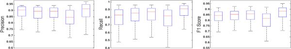
Box plot for quantitative comparison (precision, recall, and F1 score). In each panel, x-axis denotes 5 shape models (from left to right): MSM, PCA, KSVD, LASSO, and Our method.

Running Time Analysis

The Matlab execution time of this novel algorithm depends on M in (8). We evaluate the execution time of the segmentation algorithm with {M = 0, 1, 2, 3, 4, 5, 6, 7, 8, 9, 10, 15, 20, 30, 60, 100} on one 704 × 704 image patch that contains N = 101 detected tumor cells, as shown in Figure 5. M = 0 corresponds to no repulsive term considered in (8). The recall is relatively high since all shapes deform independently without any repulsion until they reach the maximum number of iterations, therefore they can almost cover the whole cells. However, the precision of boundary segmentation is extremely low. The execution time is 602 seconds when M = N – 1, which represents the case that the repulsive forces from all other cells in the image are calculated. When M = 5, also used in our experiments, the execution time is 35 seconds. As shown in Figure 5, the segmentation accuracy does not have a significant variation when M > 5, since the square of distance in f(x) of (8) greatly penalizes those contours far away. Practically, one can select a proper M by providing a rough estimation to speed up the algorithm instead of using M = N – 1.

Fig. 5.

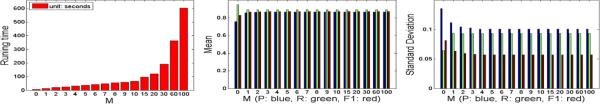
The performance with respect to the number of nearest neighbors M.

4 Conclusion

In this work, we present a novel cellular image segmentation algorithm for lung cancer, which combines the bottom-up image appearances with top-down shape priors. The shape repository is learned with a novel locality-constrained, selection-based dictionary learning algorithm, and a local repulsive balloon snake is proposed for adaptive shape deformation.

References

- 1.Aharon M, Elad M, Bruckstein A. K-SVD: an algorithm for designing over-complete dictionaries for sparse representation. TSP. 2006;54(11):4311–4322. [Google Scholar]
- 2.Al-Kofahi Y, Lassoued W, Lee W, Roysam B. Improved automatic detection and segmentation of cell nuclei in histopathology images. TBME. 2010;57(4):841–852. doi: 10.1109/TBME.2009.2035102. [DOI] [PubMed] [Google Scholar]
- 3.Ali S, Madabhushi A. An integrated region-, boundary-, shape-based active contour for multiple object overlap resolution in histological imagery. TMI. 2012;31(7):1448–1460. doi: 10.1109/TMI.2012.2190089. [DOI] [PubMed] [Google Scholar]
- 4.Chang H, Han J, Spellman PT, Parvin B. Multireference level set for the characterization of nuclear morphology in glioblastoma multiforme. TBME. 2012;59(12):3460–3467. doi: 10.1109/TBME.2012.2218107. [DOI] [PMC free article] [PubMed] [Google Scholar]
- 5.Cheng J, Rajapakse JC. Segmentation of clustered nuclei with shape markers and marking functions. TBME. 2009;56(3):741–748. doi: 10.1109/TBME.2008.2008635. [DOI] [PubMed] [Google Scholar]
- 6.Cohen LD. On active contour models and balloons. CVGIP: Image Understanding. 1991;53(2):211–218. [Google Scholar]
- 7.Cootes TF, Taylor CJ, Cooper DH, Graham J. Active shape models-their training and application. CVIU. 1995;61(1):38–59. [Google Scholar]
- 8.ElBaz MS, Fahmy AS. Active shape model with inter-profile modeling paradigm for cardiac right ventricle segmentation. MICCAI. 2012;7510:691–698. doi: 10.1007/978-3-642-33415-3_85. [DOI] [PubMed] [Google Scholar]
- 9.Freund Y, Schapire RE. A decision-theoretic generalization of on-line learning and an application to boosting. J. Comput. Syst. Sci. 1997;55(1):119–139. [Google Scholar]
- 10.Grady L, Schwartz EL. Isoperimetric graph partitioning for image segmetentation. TPAMI. 2006;28(1):469–475. doi: 10.1109/TPAMI.2006.57. [DOI] [PubMed] [Google Scholar]
- 11.Kong H, Gurcan M, Belkacem-Boussaid K. Partitioning histopathological images: an integrated framework for supervised color-texture segmentation and cell splitting. TMI. 2011;30(9):1661–1677. doi: 10.1109/TMI.2011.2141674. [DOI] [PMC free article] [PubMed] [Google Scholar]
- 12.Qi X, Xing F, Foran DJ, Yang L. Robust segmentation of overlapping cells in histopathology specimens using parallel seed detection and repulsive level set. TBME. 2012;59(3):754–765. doi: 10.1109/TBME.2011.2179298. [DOI] [PMC free article] [PubMed] [Google Scholar]
- 13.Scott DW. Parametric statistical modeling by minimum integrated squared error. Technometrics. 2001;43:274–285. [Google Scholar]
- 14.Shi Y, Qi F, Xue Z, Chen L, Ito K, Matsuo H, Shen D. Segmenting lung fields in serial chest radiographs using both population-based and patient-specific shape statistics. TMI. 2008;27(4):481–494. doi: 10.1109/TMI.2007.908130. [DOI] [PubMed] [Google Scholar]
- 15.Wang J, Yang J, Yu K, Lv F, Huang T, Gong Y. Locality-constrained linear coding for image classification. CVPR. 2010:3360–3367. [Google Scholar]
- 16.Wilms M, Ehrhardt J, Handels H. A 4D statistical shape model for automated segmentation of lungs with large tumors. MICCAI. 2012:347–354. doi: 10.1007/978-3-642-33418-4_43. [DOI] [PubMed] [Google Scholar]
- 17.Wu Z, Gurari D, Wong JY, Betke M. Hierarchical partial matching and segmentation of interacting cells. MICCAI. 2012;7510:389–396. doi: 10.1007/978-3-642-33415-3_48. [DOI] [PubMed] [Google Scholar]
- 18.Zhan Y, Dewan M, Zhou XS. Cross modality deformable segmentation using hierarchical clustering and learning. MICCAI. 2009:1033–1041. doi: 10.1007/978-3-642-04271-3_125. [DOI] [PubMed] [Google Scholar]
- 19.Zhang S, Zhan Y, Metaxas DN. Deformable segmentation via sparse shape representation and dictionary learning. MIA. 2012;16(7):1385–1396. doi: 10.1016/j.media.2012.07.007. [DOI] [PubMed] [Google Scholar]