Sparse modeling of spatial environmental variables associated with asthma

Abstract

Geographically distributed environmental factors influence the burden of diseases such as asthma. Our objective was to identify sparse environmental variables associated with asthma diagnosis gathered from a large electronic health record (EHR) dataset while controlling for spatial variation. An EHR dataset from the University of Wisconsin’s Family Medicine, Internal Medicine and Pediatrics Departments was obtained for 199,220 patients aged 5–50 years over a three-year period. Each patient’s home address was geocoded to one of 3,456 geographic census block groups. Over one thousand block group variables were obtained from a commercial database. We developed a Sparse Spatial Environmental Analysis (SASEA). Using this method, the environmental variables were first dimensionally reduced with sparse principal component analysis. Logistic thin plate regression spline modeling was then used to identify block group variables associated with asthma from sparse principal components. The addresses of patients from the EHR dataset were distributed throughout the majority of Wisconsin’s geography. Logistic thin plate regression spline modeling captured spatial variation of asthma. Four sparse principal components identified via model selection consisted of food at home, dog ownership, household size, and disposable income variables. In rural areas, dog ownership and renter occupied housing units from significant sparse principal components were associated with asthma. Our main contribution is the incorporation of sparsity in spatial modeling. SASEA sequentially added sparse principal components to Logistic thin plate regression spline modeling. This method allowed association of geographically distributed environmental factors with asthma using EHR and environmental datasets. SASEA can be applied to other diseases with environmental risk factors.

INTRODUCTION

While there is continued interest in associating genes with disease using methods such as genome-wide association studies [1], approximately 23% of disease burden and death can be attributed to environmental factors [2]. It is important to associate diseases with a strong environmental component, including respiratory infections, cardiovascular disease, cerebrovascular disease, and asthma [2], with geographical environmental factors. Methods that consider spatial variation and interpretability of results will increasingly be utilized as clinical, environmental, and geographical datasets become more readily available. Our paper applies sparsity with spatial modeling to study the association of environmental factors and asthma.

1.1 Asthma risk factors

Asthma is a chronic respiratory disease with variable and recurring symptoms, airflow obstruction, bronchial hyperresponsiveness, and inflammation [3]. Its prevalence rose by 15% in the last 10 years [4]. Based on a Wisconsin Department of Health Services asthma surveillance report, approximately 14% of adults and 10% of children have been diagnosed with asthma in Wisconsin [5]. In 2009, 5,300 people were hospitalized and 21,000 went to an emergency department with a principal diagnosis of asthma. Eleven percent of adults with asthma had an emergency department visit and 20% had urgent care visits for symptoms [5].

Asthma onset is associated with multiple, complex factors. While some are non-modifiable such as sex and age [6], many others are associated with the environment and residential location. These include educational attainment, household income, health insurance, smoking, physical activity, and obesity [6]. Medical conditions influenced by the environment and associated with asthma include atopy [7], allergic reactions [8], airway hyperreactivity [9], and airway responsiveness [10]. Over 370 outdoor and indoor environmental factors have been associated with asthma including substances from building materials, cleaning products, personal care products, central heating systems, maintenance, and humidification devices [11].

1.2 Geographical analysis of asthma

Geographic information system (GIS) analyses have been used to study geographic environmental variables associated with asthma. The most studied variable was air pollution [12], which has been measured via passive measurement, direct measurement, proximity to roadways, and traffic carbon emissions. Besides air pollution, asthma was associated with climate differences [13], latitude [14], and socioeconomic status [15]. Socioeconomic status, specifically male employment, was positively associated with asthma in a Southern California study, where access to care and the hygiene hypothesis—the idea that limited exposure to bacterial and viral pathogens during childhood result in a predisposition to allergy [16,17]—were proposed as explanations.

Fewer asthma studies have incorporated local environmental variables aggregated at the level of census tracts or block groups. Census tracts and block groups are geographic areas developed by the United State Census Bureau and contain 1,500–8,000 and 600–3,000 people, respectively. Using census tract data, asthma diagnosis was correlated with houses facing highway intersection [18] and sociodemographic characteristics of race, sex, and education [19]. Fewer studies have used block group level variables. Socioeconomic status was associated with asthma diagnosis using block group level data [15]. Many of these analyses used questionnaire data to determine asthma diagnosis, which may be limited by self-report bias [20]. These analyses involved less than 5700 participants, 10 environmental variables, and census geographic regions from only a portion of a state.

1.3 Environmental variables associated with EHR data

Environmental variables and built environments have been studied using EHR data. For example, nitrogen oxides were tested for association with diseases including asthma diagnoses obtained from EHR datasets in primary care [21]. Body mass index (BMI) calculated from EHR data was positively associated with the number of fast food restaurants near a person’s home [22].

Schwartz et al. [23] used an EHR dataset, environmental community-level variables, and multilevel statistical analysis to demonstrate that lower BMI was associated with higher socioeconomic status and areas with more venues for physical activity.

1.4 Spatial Statistics to Study Disease

Spatial statistics offer methods to incorporate geographic location to identify risk factors associated with disease [24]. The spatial statistics utilized in this study included a generalized additive model. Generalized additive models [25] are generalized linear models with predictors that involve a linear sum of smooth functions.

Previous health studies that utilized spatial generalized additive models investigated the association of air pollution and mortality, tuberculosis drug resistance patterns in Peru [26], and geographic distribution of heart disease [27].

Spatial statistics, specifically additive models, have been combined with sparsity. COSSO [28] and SpAM [29] extended the lasso estimator [30] while another approach created a new sparsity-smoothness penalty [31].

1.4 Objective

Our goal was to identify an interpretable set of environmental risk factors of asthma distributed geographically. Other studies have combined environmental variables and EHR data, spatial statistics and disease, and spatial statistics and sparsity. Our main contribution is the addition of sparsity to spatial statistics. As applied to geographically distributed EHR and environmental datasets, we describe this methodology as Sparse Spatial Environmental Analysis (SASEA).

MATERIAL AND METHODS

2.1 Source of Clinical Data

Our research group developed the University of Wisconsin Electronic Health Record - Public Health Information Exchange (UW eHealth-PHINEX), an EHR data exchange between University of Wisconsin (UW) Departments of Family Medicine, Internal Medicine, and Pediatrics and the Wisconsin Division of Public Health. Further details have been described previously [32]. Briefly, the database contains clinical care variables such as disease diagnoses, medications, and laboratory test results. Patient home addresses from year 2012 were geocoded to year 2000 block groups, the smallest geographic area the US Census Bureau publishes. Block groups were linked to detailed demographic and environmental data from the ESRI Business Analyst database [33]. The data exchange is a HIPAA Privacy Rule compliant-limited dataset, and the Wisconsin Division of Public Health is blinded to patient/provider specific information. All patient identifiers were removed from the data except birth month and year, ZIP code, and census block group of the patient’s address. Random accession numbers were used for patients, primary care providers, and clinics. This study was approved by the UW Institutional Review Board protocol M2009-1273 and UW Health with data use agreements.

UW Departments of Family Medicine, Internal Medicine and Pediatrics provide care in 42 clinics throughout Wisconsin, but most are located in southcentral Wisconsin. Patients represent various environmental and socioeconomic strata in rural and urban regions.

The dataset study period was from 2007–2009. Patients were identified as asthma cases when an asthma ICD-9 code of 493.xx was associated with a Current Procedural Terminology (CPT) codes for hospital discharges (CPT codes 99238 and 99239) or office visits (CPT codes 99201–99205 and 99211–99215). Patients were identified as controls if they did not have a hospital discharge or office visit associated with an asthma ICD-9 code over the study period, but were seen at least once in the UW Departments of Family Medicine, Internal Medicine, or Pediatrics. Participants in the study were restricted to be 5 to 50 years of age. There were no additional exclusion criteria.

This study included 199,220 participants [32]. There were 103,690 patients living in 2,186 block groups with sufficient data also linked with ESRI data to perform the analysis described in section 2.3.

The ESRI Business Analyst environmental database [33] consisted of 1,117 variables, which included demographics (age, income, education), living conditions (household members, rental property, pets, rural living), behaviors (food consumption, transportation, smoking, television), health (drug prescriptions), and businesses (types of employees and employers). Most variables (992 of the 1,117) represented data from year 2010 while the remaining variables represented data from the year 2000 (please see Appendix Table 1). Variables were normalized to the number of participants or number of households when appropriate and standardized to (0,1).

2.2 Spatial Variation of Asthma

The large-scale spatial variation of asthma was estimated using a Logistic generalized additive model with a thin plate regression spline smoothing term [34], which we refer to as a Logistic thin plate regression spline model. As described in the Introduction, generalized additive models [25] are generalized linear models with predictors that involve a linear sum of smooth functions. Smooth functions allow a more flexible model specification that can account for the spatial location of variables. A thin plate regression spline is considered an optimal smooth function as it was developed for optimal smoothness and data fitting using a more computationally feasible low rank approximation [34]. Thin plate regression splines do not require user-specified locations of knots and are multivariate, penalized low rank approximations of a smooth function with optimal data fitting and smoothness [34]. Tensor product smooths were not used as both longitude and latitude were scaled similarly. The geographic area of Wisconsin was small and did not necessitate pseudosplines on a sphere [35]. The thin plate regression spline was represented by a bivariate smooth term with the longitude and latitude of the block group centroid.

ArcGIS software [36] was used to map the total number of patients, prevalence, and Logistic thin plate regression spline modeling predicted prevalence per block group. Block groups with ≤ 20 total participants (asthmatic and non-asthmatic) were mapped with a different coloring scheme than block groups with > 20 total participants.

2.3 Association of environmental variables with asthma

The Logistic thin plate regression spline model with covariates was:

$$log({\mathit{asthma}}_{i,j})=f(x_i,y_i)+{\alpha }_j{\mathit{block}}_j+{\beta }_1{\mathit{age}}_i+{\beta }_2{\mathit{sex}}_i+{\beta }_3{\mathit{race}}_i+{\beta }_4{\mathit{ethnicity}}_i+{\beta }_5{(\mathit{BMI})}_i+{\beta }_6{(\mathit{encounter}\mathit{days})}_i+{\beta }_7{(\mathit{distance})}_i$$ (1)

where i is a participant and j is the block group participant i’s home address is geocoded to. The thin plate regression spline is $f(x_i,y_i)={\sum }_{k=1}^q{c}_k(x_i,y_i){\mathit{\zeta }}_k$ where c_k(x_i, y_i) is the k^th basis function, ζ_k is an unknown parameter, and x_i and y_i are the latitude and longitude for the centroid of the block group participant’s geocoded home address. α_jblock_j is the block group random effect allowing for hierarchical0 structuring of the model. The basis dimension, q, was chosen to be 80, which was twice the estimated degrees of freedom to allow for appropriate smoothness. BMI was the body mass index at first encounter. The encounter days covariate was defined as the number of days between a patient’s first and last encounter in the EHR dataset. Encounter days controlled for the differences between patients who utilized the University of Wisconsin’s hospitals and clinics over a short amount of time (e.g., those who had one visit to the emergency department) versus patients who utilized the hospitals and clinics over a longer amount of time (e.g., those who received the majority of their medical care at the University of Wisconsin). The distance covariate was defined as the Euclidean distance between a patient’s home address and the address of the primary care office with the most frequent visits.

An adapted Logistic generalized additive model fitting with subsampling for smoothing spline fitting was used to accommodate the large dataset [37,38]. Subsampling was a technique used for faster computation and did not cause parameter estimate variability. The smoothing splines were first set using a subsample of the data. In each subsequent step of the penalized iteratively re-weighted least squares (PIRLS) algorithm, the weighted model matrix was constructed in blocks with the corresponding QR decomposition so as not to form the entire model matrix. This method is justified for restricted maximum likelihood estimation because of asymptotic multivariate normality of Q’z, where z is the pseudodata. This adapted method was previously implemented in the R package mgcv using the bam function with tp parameter [34].

The 1,117 environmental variables from ESRI were dimensionally reduced using sparse principal component analysis (SPCA) [39] before testing for association with asthma. SPCA is in contrast to principal component analysis (PCA). In PCA, the principal components are a linear combination of the original variables. SPCA uses only a small number of non-zero weighted original variables to create each principal component. By having a small number of the original variables constitute each principal component, we can more easily discuss groupings of variables. The simplest SPCA implementation first identifies principal components with traditional PCA. Each principal component can then be regressed using the original variables with a lasso penalty. We chose twenty as the number of non-zero variables to be included for each sparse principal component for ease of interpretability. The SPCA algorithm determined which environmental variables were chosen. We utilized the spca function in the elasticnet package from R [39].

The sparse principal components were used to determine how environmental variables were associated with asthma. Starting with the first sparse principal component, which represented the greatest variance of the ESRI dataset, sparse principal components were added sequentially to the Logistic thin plate regression spline model with covariates as shown below.

$$log({\mathit{asthma}}_{i,j})=f(x_i,y_i)+{\alpha }_j{\mathit{block}}_j+{\beta }_1{\mathit{age}}_i+{\beta }_2{\mathit{sex}}_i+{\beta }_3{\mathit{race}}_i+{\beta }_4{\mathit{ethnicity}}_i+{\beta }_5{(\mathit{BMI})}_i+{\beta }_6{(\mathit{encounter}\mathit{days})}_i+{\beta }_7{(\mathit{distance})}_i+{\sum }_{m=1}^r{\delta }_m{(\mathit{SPC})}_{j,m}$$ (2)

where r = {1, …, 18} and (SPC)_j,m is the value of sparse principal component m at block group j. The largest model tested included the thin plate regression spline, covariates, and sparse principal components one through eighteen. Bayesian Information Criterion (BIC) was used to compare models without sparse principal components and with r = {1, …, 18}. Eighteen was chosen as the maximum number of sparse principal components we would be willing to investigate, as interpretability of environmental variables was a major goal. As models with increasing parameters can have a greater likelihood, BIC is a score used in model selection that penalizes the likelihood by the number of parameters. BIC = −2 * ln(L) + k * ln(N), where L is the likelihood, k is the number of parameters estimated and N is the number of observations [40]. The model with the lowest BIC is optimal.

We summarize the number of variables used in modeling. There are 1,117 environmental variables. Using sparse principal components analysis, 20 environmental variables were selected to represent each sparse principal component (SPC). By using SPCA, SPCs were ranked by importance based on the variance each SPCs represented from the original environmental variable dataset. To determine which SPCs to add to the model, we added the SPCs in order from rank #1 to rank #18. For example, we tested if the model was best fit if SPC 1 was added; if SPC 1 and 2 were added; if SPC 1, 2, and 3 were added; etc…; and if SPC 1 through 18 were added. The model also included 6 non-environmental covariates to control for variables that likely affect asthma diagnosis.

The change in log odds of asthma diagnosis per unit measure of sparse principal component m, δ_m(SPC)_j,m, was examined for each Wisconsin block group j. As ${(\mathit{SPC})}_j={\sum }_{n=1}^{20}{\eta }_n{(EV)}_n$ where EV is an environmental variable from the ESRI database, the associated effect on the change in log odds of asthma diagnosis for an individual environmental variable could be assessed via the sign of η_n and η_m. All statistical analyses were performed in R.[34,41]

The graphical abstract summarizes the SASEA methods integrated in this study. We began with electronic health record data (covariates, asthma diagnosis as defined above, and the block group participants resided in) and environmental variables from Esri (values represent measurements from a block group). We applied sparse principal component analysis to the environmental variables. We combined the EHR dataset with the sparse principal components from the environmental variable dataset. We ran a logistic thin plate regression spline model on this combined dataset. Bayesian information criterion was used to select the number of sparse principal components added to the model. The odds ratios for variables in the logistic regression model were reported. The change in log odds value was color coded and mapped to block groups.

RESULTS

Figure 1a shows major cities and population by county in Wisconsin. Figure 1b shows the total number of patients from the EHR dataset per block group. The majority of patients were in Dane County, WI and eight southern counties. Most participants were near the four, more urban cities including Madison, Eau Claire, Wausau, and Appleton. The median and maximum number of participants per block was 5 and 2,673, respectively. 927 out of 3,307 block groups had greater than 20 total participants. The asthma period prevalence from 2007–2009 was 8.4% (16,739 out of 199,220).

Figure 1. Major Cities and County Population in Wisconsin and Total Number of Participants Per Block Group from UW eHealth-PHINEX.

Major Wisconsin cities and population by county (a) and the total number of participants per block group in UW eHealth-PHINEX (b) are shown. White block groups do not contain any patient data. The light yellow block groups in (b) correspond to block groups with ≤ 20 total participants.

Figure 2 shows asthma prevalence and the Logistic thin plate regression spline model predicted prevalence for each block group using only a coordinate bivariate smooth term, log(asthma_i,j) = f(x_i, y_i) + ε_i,j. The median and maximum prevalence estimates were 0% and 100%, which was expected as many block groups had a low total number of participants (Figure 3a). However, the regression model was intended to smooth prevalence and decrease extreme values (Figure 3b). The predicted prevalence had a minimum, median, and maximum prevalence of 2.3%, 6.8%, and 12%. Spatially, higher prevalence was modeled in the urban southcentral, rural southwestern, and central regions of the state. Lower prevalence was modeled in rural areas of the state.

Figure 2. Asthma Prevalence and Logistic Thin Plate Regression Spline Model Predicted Prevalence.

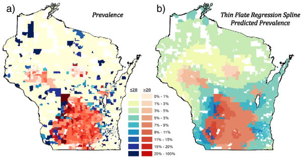
Asthma prevalence (a) and Logistic thin plate regression spline model predicted prevalence (b). The Logistic model only contains the thin plate regression spline smooth term. Two color maps are used to highlight areas of less or more confidence: blue for block groups with ≤ 20 participants and red for block groups with > 20 total participants. White block groups do not contain any patient data. As intended, the regression model creates a smoother spatially predicted prevalence and decreases extreme values, resulting in more moderate (less extremely dark and extremely light) blue and red coloring.

Figure 3. Spatial Change in Log Odds for Sparse Principal Components 2 and 4.

The change in log odds of asthma diagnosis per unit measure of sparse principal components 2 and 4 is shown at each block group. White represents a change in log odds between 0 and 0.01. The blue gradient represents a change in log odds <0, and the red gradient represents a change in log odds >0.01. There was a positive change in log odds of asthma diagnosis in rural areas while there was a negative change in log odds in the urban areas of Madison and Milwaukee for sparse principal component 2 (a). There was a positive change in log odds of asthma diagnosis in eastern areas of Wisconsin (b).

The Logistic thin plate regression spline model with covariates had the lowest BIC when four sparse principal components were added to the model (56,511) compared with the model containing no sparse principal components (63,974) or 2–3 and 5–18 sparse principal components (56,528–56,581). The four sparse principal components accounted for 0.9%, 0.7%, 0.5% and 0.2% of the variance from the original dataset. The odds ratios of asthma diagnosis for covariates and the four sparse principal components are shown in Table 1. Race had the greatest effect size. The odds of asthma diagnosis for black participants were highest at 1.78 (1.63–1.94) compared with the odds of asthma diagnosis for white participants. The odds of asthma diagnosis for Asian participants were lowest at 0.66 (0.57–0.77) compared with the odds of asthma diagnosis for white participants. Hispanic ethnicity compared to non-Hispanic ethnicity and age per 10 years had a moderate decrease in the odds ratio of asthma diagnosis. Sex, encounter days, and distance to clinic had no or smaller effect size on asthma diagnosis odds ratio. Of the sparse principal components, sparse principal components 2 with an odds ratio of 0.95 (0.89–0.99) and 4 with an odds ratio of 1.13 (1.01–1.27) were significant. The range of data values for sparse principal components 1, 2, 3, and 4 was 30.9, 14.4, 21.1, and 10.6, respectively.

Table 1.

Odds ratios for variables in the Logistic thin plate regression spline model

	OR (95% CI)
Sex
Male	reference
Female	1.00 (0.96, 1.05)
Age (per 10 years)	0.84 (0.82, 0.85)
Race
White	reference
Black	1.78 (1.63, 1.94)
Asian	0.66 (0.57, 0.77)
American Indian	1.25 (1.00, 1.56)
Hawaiian or Pacific Islander	1.29 (0.77, 2.18)
Unknown	0.81 (0.68, 0.96)
Ethnicity
Non-Hispanic	reference
Hispanic	0.79 (0.69, 0.90)
Unknown	0.81 (0.68, 0.96)
BMI (per 5 kg/m2)	1.18 (1.16, 1.20)
Encounter days in EHR dataset (per 30 days)	1.05 (1.04, 1.05)
Distance to clinic (per 10 mile)	1.02 (1.00, 1.03)
Sparse Principal Component 1 (per 5 units)	1.00 (0.96, 1.05)
Sparse Principal Component 2 (per 5 units)	0.95 (0.89, 0.99)
Sparse Principal Component 3 (per 5 units)	0.94 (0.86, 1.03)
Sparse Principal Component 4 (per 5 units)	1.13 (1.01, 1.27)

OR, odds ratio, CI, confidence interval, BMI, body mass index, EHR, electronic health record Age, BMI, encounter days in EHR, distance to clinic, and sparse principal component odds ratios are scaled by 10 years, 5 kg/m², 30 days, 10 miles, and 5 units, respectively

Table 2 shows representative, high loading environmental variables of the four sparse principal components. Variable loadings and model coefficients are shown as well. Variables of significant sparse principal components with positive loadings and positive model coefficients, including households with disposable income less than $15,000, were positively associated with asthma. Variables of significant sparse principal components with negative loadings and negative model coefficients, including renter occupied housing units, were positively associated with asthma. Variables of significant sparse principal components with positive loadings and negative model coefficients, including dog ownership, were negatively associated with asthma (please see Appendix Table 2 for all variables and loadings of these four sparse principal components).

Table 2.

Representative Variables from Sparse Principal Components

Sparse Principal Component	Variable	SPC Loading	Model Coefficient (δ)
1	Food at Home: Average	0.36	6.1×10−4
2	Household owns 1 dog	0.49	−1.1×10−2
	Renter Occupied Housing Units	−0.41
3	Average Household Size	0.51	−1.2×10−2
4	Households with Disposable Income less than $15,000	0.76	2.5×10−2

SPC, sparse principal component

The change in log odds of asthma diagnosis per unit measure of sparse principal components 2 and 4 are shown in Figure 3. The change in log odds was calculated for sparse principal component m, Wisconsin block group j, and model coefficient δ as δ_m(SPC)_j,m. The urban areas of Wisconsin include Madison, Milwaukee, Eau Claire, La Crosse, and Appleton, whose locations are shown in Figure 2a. For sparse principal component 2, rural areas of the state had a positive change in log odds of asthma diagnosis (Figure 3a). The two southern urban areas with a negative change in log odds included Madison and Milwaukee. As the SPC loading for dog ownership was positive and the model coefficient of SPC 2, δ₂, was negative (Table 2), less dog ownership contributed to the positive change in log odds of asthma diagnosis in rural areas. As the SPC loading for renter occupied housing units was negative (Table 2), more renter occupied housing units contributed to the positive change in log odds of asthma diagnosis in rural areas. For sparse principal component 4, eastern areas of the state had a positive change in log odds of asthma diagnosis (Figure 3b). As the SPC loading for households with a disposable income less than $15,000 was positive and the model coefficient of SPC 4 δ₄, was positive (Table 2), more households with a disposable income less than $15,000 contributed to the positive change in log odds of asthma diagnosis in eastern Wisconsin.

DISCUSSION

It is estimated that the lack of medical care accounts for 10 percent of early deaths in the United States. The remaining determinants of health contributing to early deaths include genetics, social circumstances, environmental exposure, and behavioral patterns [42]. Our work utilizing SASEA is unique in the application of sparsity to spatial statistics. We use of a large EHR dataset to identify sparse environmental variables associated with asthma. This methodology was able to identify several location-specific, environmental risk factors associated with asthma. Specifically, less dog ownership and more renter occupied housing units were associated with increased asthma in rural areas. More households with low disposable income were associated with increased asthma in eastern Wisconsin.

4.1 SASEA

We attempted to account for multiple comparisons of the many variables and identify a smaller set of interpretable risk factors. The SASEA method performs sparse principal component analysis outside of the regression model as a means to prevent overfitting. Twenty non-zero loading variables for each sparse principal component were chosen to consider small groups of variables. Sparse principal components were sequentially added using BIC for model selection given the greater variance represented by higher ranked components. The sequential addition allowed for further structured and sparse variable evaluation. Although a set of sparse principal components were selected by BIC (four in this study), only some may be significant based on the odds ratio (two in this study). This feature of SASEA enhances sparsity as well.

The integrations of various scalable methods accommodated analysis of the EHR, environmental, and geographical datasets. Use of adaptable statistical model fitting based on well-studied algorithms was an asset that allowed for simple extension to the large number of patients and variables.

4.2 Community variables associated with asthma

Similarly to our study, two additional studies [14,15] investigated community environmental variables associated with asthma. In our study, asthma was defined based on EHRs compared to survey data in the other two studies [14,15]. Many variables overlapped among these three studies. Our study and Krstić’s study [14] used latitude and longitude. We did not use insolation, air temperature or air pollution. Shankardass et al. [15] and our study had the individual variables of age, race, gender, and BMI. Shankardass et al. [15] included more individual variables including freeway distance while our study included more community environmental variables. We did not have male unemployment, which Shankardass et al. [15] found significantly associated with asthma. However we had other variables similar to socioeconomic status such as disposable income and employed civilian population in sparse principal components.

For analyses, Krstić [14] used linear regression, Shankardass et al. [15] used multilevel logistic random effect modeling, and our study used logistic thin plate regression spline modeling. The random effect modeling likely was more applicable to Shankardass et al. [15] as communities were concentrated. In our study the random effect in addition to thin plate regression spline based on latitude and longitude was chosen because of the distribution of patients throughout the state of Wisconsin.

4.3 Sparse principal components associated with asthma

As seen in other studies [6,40], higher asthma prevalence was associated with increased BMI, female sex, and black race, while lower asthma prevalence was associated with Hispanic ethnicity. Age, encounter days in the EHR dataset, and distance to most frequented clinic had little association with asthma diagnosis. Sparse principal component 2 represented by dog ownership and renter occupied housing units in addition to sparse principal component 4 represented by disposable income less than $15,000 were significantly associated with asthma. The individual variables representing sparse principal components likely contributed a small effect size.

Previous studies support the association of asthma and the environmental variables representing the sparse principal components in this study. In this study, dog ownership had a negative association with asthma. Other studies have shown perinatal and early life exposure to dog allergen was associated with reduced allergy and asthma risk later in life [43,44]. Renter occupied housing units were positively associated with asthma in a Brazil study [45]. Rental housing was associated with cold and damp housing, which in turn were associated with increased asthma [46]. Lastly, lower socioeconomic status as reflected by disposable income less than $15,000 was associated with greater asthma. Previously mentioned studies came to similar conclusion [5,6]. However, these results contradicted the positive association of socioeconomic status with asthma found in the Shankardass et al. [15]. Thus, the SASEA method used in this study identified variables that were previously associated with asthma risk, suggesting that these methods may have a role to studying chronic disease.

Mapping the associated change in log odds of asthma for a sparse principal component highlighted the geographic distribution of these sparse principal components and high loading environmental variables. The urban and rural discrepancy seen in differences in renter occupied housing units may be driven by the built environment, the human-made space where people live and work [47].

4.4 EHR as a measure of clinical data

The use of EHR and block group characteristics merits comparison with traditional forms of health surveys including self-report and public health measured data. Canadian studies suggested census aggregate-level measures of income and education did not approximate individual level measures well [48–51]. There was similarity between self-reported variables and clinically measured variables. Self-reported colon cancer screening was similar to EHR imputed data [52]. Public health measured data were similar to EHR measured data. For example, BMI-based childhood obesity was 18% in both an EHR dataset and the National Health and Nutrition Evaluation Survey [53].

Agreement between disease prevalence based on health surveys and disease prevalence based on EHR datasets varies depending on disease. EHR datasets had prevalence similar to that from surveys for test-based conditions (e.g. diabetes) and decreased prevalence for minor conditions (e.g. back pain, headache, skin conditions) [54–56]. Specifically, two Spanish studies showed that the asthma prevalence calculated from an EHR dataset was lower compared with asthma prevalence calculated from population surveys [54,55]. However asthma prevalence based on UW eHealth-PHINEX (8.4%) was similar to the Wisconsin health survey, Behavioral Risk Factor Surveillance System (8.0%) [20]. As there is no single lab test for diagnosis of asthma, ICD-9 codes likely under-identify asthma when compared with “gold standard” manual record review [57] but may be more objective compared with population surveys.

CONCLUSIONS

5.1 Future work and alternative methods

Further analysis to determine the individual variables from sparse principal components that are associated with asthma could be performed using traditional methods such as stepwise model selection with BIC. This analysis could be performed with UW eHealth-PHINEX data from other years (e.g. 2009–2012), a UW eHealth-PHINEX hold out dataset, or a non-UW eHealth-PHINEX EHR dataset in another geographic region.

There are many future directions for this work regarding diseases and methods. Our methods could be applied to asthma control, other chronic diseases, and different communities. The census block groups and ESRI environmental data are already available nationwide. It is foreseeable that with the integration of a national EHR dataset, this type of analysis will be utilized to identify spatial risk factors to allow investigation or evaluation of interventions in any geographic region [58].

Alternative methods could have been used in this study. Traditional Logistic regression without the smoothing term does not account for the unknown orientation of spatial correlation among asthma due to geography, nor does it directly address difficulties in high dimensional data by constructing sparse models. Other spatial models included conditional auto-regressive models ^[59]. As the four sparse principal components accounted for a small percentage of variance from the original dataset, other methods such as traditional principal components analysis or clustering could have been utilized. However, traditional principal component analysis maintained all variables in each principal component preventing sparse interpretation, and clustering environmental variables added complexity. Few variables could have been associated more directly with the Logistic thin plate regression spline model using least absolute shrinkage and selector operator [30] such as COSSO [28]. However, a new set of variables would be identified for different diseases and variables could not be grouped. Allowing regression coefficients to vary over space as in geographically weighted regression [60] could be accomplished with spatial smoothing spline interaction terms.

5.2 Limitations

There were limitations to the study. Although measures were taken to prevent overfitting and accommodate high dimensionality, this was an ecological, data-mining study without a priori variable hypotheses. This additive non-linear model likely does not fully capture the complexity of environmental factors influencing asthma.

The associations noted in the study may be due to confounding factors. One must be cognizant of ecological bias, because results about groups of people do not necessarily translate to the same findings about individuals. However, the neighborhood in which an individual lives in has been associated with health outcomes [61].

Multiple studies have shown the importance of EHR disease phenotype definitions, algorithm development, and validation [62–64]. In this study, asthma cases were defined based on ICD-9 codes. Some have argued this may under-estimate asthma prevalence [57]. Aside from this study’s EHR asthma phenotype definition, which is similar to the validated definition of Gershon et al. [65], other definitions such as the Healthcare Effectiveness Data and Information Set [66], have not been validated. We are currently validating alternative EHR phenotype definitions, which will also be used to segment asthma severity.

The results may be biased as UW eHealth-PHINEX data is not a complete representation of all block groups or persons in the state of Wisconsin. UW Family Medicine, Internal Medicine, and Pediatrics departments are an integrated health care system, but patients can receive care in at least two other major systems in the same catchment area. Because many hospitals and clinics have, or will soon have, an EHR system, sharing data through a statewide information exchange could mitigate this issue.

Another potential limitation is that the analysis included data elements from different years. While the EHR dataset represented years 2007–2009, the patient addresses were from the date of EHR data extraction in year 2012. However, compared with other states, Wisconsin residents tend to move less frequently. Wisconsin is the fifth “stickiest” state, with 68.6% of the current residents having been born in Wisconsin, an indicator of decreased residential mobility [67]. Patient addresses were geocoded to year 2000 block groups to match the ESRI database. ESRI database variables were mostly from year 2010, while some census variables were from year 2000. There is minimal change in block group from year to year and the goal was to identify general trends of larger geographic areas. The ESRI year 2010 variables were closest to the EHR database dates and the census year 2010 variables were not yet available.

Our main contribution is the incorporation of sparsity in spatial modeling. The sequential addition of sparse principal components to Logistic thin plate regression allowed interpretable analysis of geographically distributed EHR and environmental datasets. Understanding spatial disease variation and environmental risk factors using methods such as SASEA can allow better explanation of geographical disease disparity.

HIGHLIGHTS.

• We geocode patients from an electronic health record to their corresponding block group.

• We identify sparse environmental variables associated with asthma considering spatial variation.

• Sparse principal component analysis and logistic thin plate regression splines were utilized.

• Dogs and rental housing were associated with asthma in specific regions.

Abbreviations

UW eHealth-PHINEX

University of Wisconsin Electronic Health Record – Public Health Information Exchange

EHR

electronic health record

APPENDIX A. Supplementary material

Supplementary data associated with this article can be found in the online version.

References

- 1.Manolio TA. Genomewide association studies and assessment of the risk of disease. N Engl J Med. 2010;363:166–76. doi: 10.1056/NEJMra0905980. [DOI] [PubMed] [Google Scholar]
- 2.Prüss-Üstün A, Corvalán C. Preventing disease through healthy environments: Towards an estimate of the environmental burden of disease. World Health Organization; 2006. [Google Scholar]
- 3.Busse WW, Boushey HA, Camargo CA, et al. National Asthma Education and Prevention Program: Expert Panel Report 3: Guidelines for the Diagnosis and Management of Asthma, Summary Report 2007. Bethesda, MD: National Institutes of Health; National Heart, Lung, and Blood Institute; 2007. [Google Scholar]
- 4.Centers for Disease Control and Prevention. [accessed 21 May2013];Asthma’s Impact on the Nation: Data From the CDC National Asthma Control Program. http://www.cdc.gov/asthma/impacts_nation/AsthmaFactSheet.pdf.
- 5.Wisconsin Department of Health Services, Division of Public Health, Bureau of Environmental and Occupational Health. [accessed 21 May2013];Burden of Asthma in Wisconsin 2010. 2012 http://www.dhs.wisconsin.gov/eh/asthma/pdf/BurdenofAsthma2010Web.pdf.
- 6.Zahran HS, Bailey C. Factors associated with asthma prevalence among racial and ethnic groups-United States, 2009–2010 Behavioral Risk Factor Surveillance System. J Asthma. doi: 10.3109/02770903.2013.794238. Published Online First: 11 April 2013. [DOI] [PMC free article] [PubMed] [Google Scholar]
- 7.Arbes SJ, Jr, Gergen PJ, Vaughn B, et al. Asthma cases attributable to atopy: results from the Third National Health and Nutrition Examination Survey. J Allergy Clin Immunol. 2007;120:1139–45. doi: 10.1016/j.jaci.2007.07.056. [DOI] [PMC free article] [PubMed] [Google Scholar]
- 8.Torrent M, Sunyer J, Garcia R, et al. Early-life allergen exposure and atopy, asthma, and wheeze up to 6 years of age. Am J Respir Crit Care Med. 2007;176:446–53. doi: 10.1164/rccm.200607-916OC. [DOI] [PubMed] [Google Scholar]
- 9.Porsbjerg C, von Linstow M-L, Ulrik CS, et al. Risk factors for onset of asthma: a 12-year prospective follow-up study. Chest. 2006;129:309–16. doi: 10.1378/chest.129.2.309. [DOI] [PubMed] [Google Scholar]
- 10.Jackson DJ, Evans MD, Gangnon RE, et al. Evidence for a causal relationship between allergic sensitization and rhinovirus wheezing in early life. Am J Respir Crit Care Med. 2012;185:281–5. doi: 10.1164/rccm.201104-0660OC. [DOI] [PMC free article] [PubMed] [Google Scholar]
- 11.Perkins+Will . Healthy Environments: A Compilation of Substances Linked to Asthma. New York, NY: 2012. [accessed 8 May2013]. http://transparency.perkinswill.com/assets/whitepapers/NIH_AsthmaReport_2012.pdf. [Google Scholar]
- 12.Patel MM, Miller RL. Air pollution and childhood asthma: recent advances and future directions. Curr Opin Pediatr. 2009;21:235–42. doi: 10.1097/MOP.0b013e3283267726. [DOI] [PMC free article] [PubMed] [Google Scholar]
- 13.Hales S, Lewis S, Slater T, et al. Prevalence of adult asthma symptoms in relation to climate in New Zealand. Environ Health Perspect. 1998;106:607–10. doi: 10.1289/ehp.98106607. [DOI] [PMC free article] [PubMed] [Google Scholar]
- 14.Krstić G. Asthma prevalence associated with geographical latitude and regional insolation in the United States of America and Australia. PLoS ONE. 2011;6:e18492. doi: 10.1371/journal.pone.0018492. [DOI] [PMC free article] [PubMed] [Google Scholar]
- 15.Shankardass K, McConnell RS, Milam J, et al. The association between contextual socioeconomic factors and prevalent asthma in a cohort of Southern California school children. Soc Sci Med. 2007;65:1792–806. doi: 10.1016/j.socscimed.2007.05.048. [DOI] [PMC free article] [PubMed] [Google Scholar]
- 16.Strachan DP. Hay fever, hygiene, and household size. BMJ. 1989;299:1259–60. doi: 10.1136/bmj.299.6710.1259. [DOI] [PMC free article] [PubMed] [Google Scholar]
- 17.Yazdanbakhsh M, Kremsner PG, van Ree R. Allergy, Parasites, and the Hygiene Hypothesis. Science. 2002;296:490–4. doi: 10.1126/science.296.5567.490. [DOI] [PubMed] [Google Scholar]
- 18.Juhn YJ, Qin R, Urm S, et al. The influence of neighborhood environment on the incidence of childhood asthma: a propensity score approach. J Allergy Clin Immunol. 2010;125:838–843. e2. doi: 10.1016/j.jaci.2009.12.998. [DOI] [PMC free article] [PubMed] [Google Scholar]
- 19.Holt EW, Theall KP, Rabito FA. Individual, Housing, and Neighborhood Correlates of Asthma among Young Urban Children. Journal of Urban Health. 2013;90:1116–29. doi: 10.1007/s11524-012-9709-3. [DOI] [PMC free article] [PubMed] [Google Scholar]
- 20.Tomasallo C, Hanrahan LP, Arndt B, et al. Estimating Wisconsin Asthma Prevalence Using Clinical Electronic Health Records and Public Health Data. Forthcoming. Am J Public Health. 2013 doi: 10.2105/AJPH.2013.301396. [DOI] [PMC free article] [PubMed] [Google Scholar]
- 21.Kelly F, Armstrong B, Atkinson R, et al. The London low emission zone baseline study. Res Rep Health Eff Inst. 2011:3–79. [PubMed] [Google Scholar]
- 22.Jilcott SB, Wade S, McGuirt JT, et al. The association between the food environment and weight status among eastern North Carolina youth. Public Health Nutr. 2011;14:1610–7. doi: 10.1017/S1368980011000668. [DOI] [PubMed] [Google Scholar]
- 23.Schwartz BS, Stewart WF, Godby S, et al. Body mass index and the built and social environments in children and adolescents using electronic health records. Am J Prev Med. 2011;41:e17–28. doi: 10.1016/j.amepre.2011.06.038. [DOI] [PubMed] [Google Scholar]
- 24.Waller LA, Gotway CA. Applied spatial statistics for public health data. 1. New York, NY: Wiley-Interscience; 2004. [Google Scholar]
- 25.Hastie T, Tibshirani R. Generalized additive models. Statistical Science. 1986;1:297–310. doi: 10.1177/096228029500400302. dx.doi.org/10.1214/ss/1177013604. [DOI] [PubMed] [Google Scholar]
- 26.Lin H-H, Shin SS, Contreras C, et al. Use of spatial information to predict multidrug resistance in tuberculosis patients, Peru. Emerging Infect Dis. 2012;18:811–3. doi: 10.3201/eid1805.111467. [DOI] [PMC free article] [PubMed] [Google Scholar]
- 27.Chaix B, Rosvall M, Lynch J, et al. Disentangling contextual effects on cause-specific mortality in a longitudinal 23-year follow-up study: impact of population density or socioeconomic environment? Int J Epidemiol. 2006;35:633–43. doi: 10.1093/ije/dyl009. [DOI] [PubMed] [Google Scholar]
- 28.Lin Y, Zhang HH. Component selection and smoothing in multivariate nonparametric regression. The Annals of Statistics. 2006;34:2272–97. doi: 10.1214/009053606000000722. [DOI] [Google Scholar]
- 29.Ravikumar P, Lafferty J, Liu H, et al. Sparse additive models. Journal of the Royal Statistical Society: Series B (Statistical Methodology) 2009;71:1009–30. doi: 10.1111/j.1467-9868.2009.00718.x. [DOI] [Google Scholar]
- 30.Tibshirani R. Regression shrinkage and selection via the lasso. Journal of the Royal Statistical Society Series B (Methodological) 1996;58:267–88. doi: 10.1111/j.1467-9868.2011.00771.x. [DOI] [Google Scholar]
- 31.Meier L, Van de Geer S, Bühlmann P. High-dimensional additive modeling. The Annals of Statistics. 2009;37:3779–821. doi: 10.1214/09-AOS692. [DOI] [Google Scholar]
- 32.Guilbert TW, Arndt B, Temte J, et al. The Theory and Application of UW eHealth-PHINEX, A Clinical Electronic Health Record–Public Health Information Exchange. Wisconsin Medical Journal. 2012;111:124–33. [PubMed] [Google Scholar]
- 33.Esri. Esri Business Analyst Desktop Premium. Redlands, CA: Environmental Systems Research Institute; 2010. [accessed 17 Jun2012]. http://www.esri.com/software/arcgis/extensions/businessanalyst/data-us-prem.html. [Google Scholar]
- 34.Wood SN. Thin plate regression splines. J R Stat Soc: Series B (Statistical Methodology) 2003;65:95–114. doi: 10.1111/1467-9868.00374. [DOI] [Google Scholar]
- 35.Wahba G. Spline interpolation and smoothing on the sphere. SIAM Journal on Scientific and Statistical Computing. 1981;2:5–16. [Google Scholar]
- 36.Esri. ArcGIS Desktop. Redlands, CA: Environmental Systems Research Institute; 2010. [Google Scholar]
- 37.Wood SN. Fast stable direct fitting and smoothness selection for generalized additive models. Journal of the Royal Statistical Society: Series B (Statistical Methodology) 2008;70:495–518. doi: 10.1111/j.1467-9868.2007.00646.x. [DOI] [Google Scholar]
- 38.Golub GH, Van Loan CF. Matrix computations 1996. Johns Hopkins University, Press; Baltimore, MD, USA: 1983. [Google Scholar]
- 39.Zou H, Hastie T, Tibshirani R. Sparse principal component analysis. J Comp Graph Stat. 2006;15:265–86. doi: 10.1198/106186006X113430. [DOI] [Google Scholar]
- 40.Schwarz G. Estimating the dimension of a model. Ann Statist. 1978;6:461–4. [Google Scholar]
- 41.R Development Core Team. R: Language and Environment for Statistical Computing. Vienna, Austria: R Foundation for Statistical Computing; 2011. http://www.R-project.org. [Google Scholar]
- 42.McGinnis JM, Williams-Russo P, Knickman JR. The case for more active policy attention to health promotion. Health Aff (Millwood) 2002;21:78–93. doi: 10.1377/hlthaff.21.2.78. [DOI] [PubMed] [Google Scholar]
- 43.Lodge CJ, Allen KJ, Lowe AJ, et al. Perinatal cat and dog exposure and the risk of asthma and allergy in the urban environment: a systematic review of longitudinal studies. Clin Dev Immunol. 2012;2012:176484. doi: 10.1155/2012/176484. [DOI] [PMC free article] [PubMed] [Google Scholar]
- 44.Smallwood J, Ownby D. Exposure to Dog Allergens and Subsequent Allergic Sensitization: An Updated Review. Current Allergy and Asthma Reports. doi: 10.1007/s11882-012-0277-0. Published Online First: 9 June 2012. [DOI] [PubMed] [Google Scholar]
- 45.Breda D, Freitas PF, Pizzichini E, et al. Prevalence of asthma symptoms and risk factors among adolescents in Tubarão and Capivari de Baixo, Santa Catarina State, Brazil. Cad Saude Publica. 2009;25:2497–506. doi: 10.1590/s0102-311x2009001100019. [DOI] [PubMed] [Google Scholar]
- 46.Butler S, Williams M, Tukuitonga C, et al. Problems with damp and cold housing among Pacific families in New Zealand. N Z Med J. 2003;116:U494. [PubMed] [Google Scholar]
- 47.Roof K, Oleru N. Public health: Seattle and King County’s push for the built environment. J Environ Health. 2008;71:24–7. [PubMed] [Google Scholar]
- 48.Marra CA, Lynd LD, Harvard SS, et al. Agreement between aggregate and individual-level measures of income and education: a comparison across three patient groups. BMC Health Serv Res. 2011;11:69. doi: 10.1186/1472-6963-11-69. [DOI] [PMC free article] [PubMed] [Google Scholar]
- 49.Demissie K, Hanley JA, Menzies D, et al. Agreement in measuring socio-economic status: area-based versus individual measures. Chronic Dis Can. 2000;21:1–7. [PubMed] [Google Scholar]
- 50.Sin DD, Svenson LW, Man SF. Do area-based markers of poverty accurately measure personal poverty? Can J Public Health. 2001;92:184–7. doi: 10.1007/BF03404301. [DOI] [PMC free article] [PubMed] [Google Scholar]
- 51.Southern DA, McLaren L, Hawe P, et al. Individual-level and neighborhood-level income measures: agreement and association with outcomes in a cardiac disease cohort. Med Care. 2005;43:1116–22. doi: 10.1097/01.mlr.0000182517.57235.6d. [DOI] [PubMed] [Google Scholar]
- 52.Palaniappan LP, Maxwell AE, Crespi CM, et al. Population Colorectal Cancer Screening Estimates: Comparing Self-Report to Electronic Health Record Data in California. Int J Canc Prev. 2011:4. [PMC free article] [PubMed] [Google Scholar]
- 53.Bailey LC, Milov DE, Kelleher K, et al. Multi-Institutional Sharing of Electronic Health Record Data to Assess Childhood Obesity. PLoS ONE. 2013;8:e66192. doi: 10.1371/journal.pone.0066192. [DOI] [PMC free article] [PubMed] [Google Scholar]
- 54.Violán C, Foguet-Boreu Q, Hermosilla-Pérez E, et al. Comparison of the information provided by electronic health records data and a population health survey to estimate prevalence of selected health conditions and multimorbidity. BMC Public Health. 2013;13:251. doi: 10.1186/1471-2458-13-251. [DOI] [PMC free article] [PubMed] [Google Scholar]
- 55.Esteban-Vasallo MD, Domínguez-Berjón MF, Astray-Mochales J, et al. Epidemiological usefulness of population-based electronic clinical records in primary care: estimation of the prevalence of chronic diseases. Fam Pract. 2009;26:445–54. doi: 10.1093/fampra/cmp062. [DOI] [PubMed] [Google Scholar]
- 56.Cricelli C, Mazzaglia G, Samani F, et al. Prevalence estimates for chronic diseases in Italy: exploring the differences between self-report and primary care databases. J Public Health Med. 2003;25:254–7. doi: 10.1093/pubmed/fdg060. [DOI] [PubMed] [Google Scholar]
- 57.Juhn Y, Kung A, Voigt R, et al. Characterisation of children’s asthma status by ICD-9 code and criteria-based medical record review. Prim Care Respir J. 2011;20:79–83. doi: 10.4104/pcrj.2010.00076. [DOI] [PMC free article] [PubMed] [Google Scholar]
- 58.Ackermann RT, Finch EA, Brizendine E, et al. Translating the Diabetes Prevention Program into the community. The DEPLOY Pilot Study. Am J Prev Med. 2008;35:357–63. doi: 10.1016/j.amepre.2008.06.035. [DOI] [PMC free article] [PubMed] [Google Scholar]
- 59.Besag J. Spatial interaction and the statistical analysis of lattice systems. Journal of the Royal Statistical Society Series B (Methodological) 1974;36:192–236. [Google Scholar]
- 60.Brunsdon C, Fotheringham S, Charlton M. Geographically weighted regression. Journal of the Royal Statistical Society: Series D (The Statistician) 1998;47:431–43. [Google Scholar]
- 61.Sampson RJ, Morenoff JD, Gannon-Rowley T. Assessing ‘neighborhood effects’: Social Processes and New Directions in Research. Annual Review of Sociology. 2002;28:443–78. doi: 10.1146/annurev.soc.28.110601.141114. [DOI] [Google Scholar]
- 62.Newton KM, Peissig PL, Kho AN, et al. Validation of electronic medical record-based phenotyping algorithms: results and lessons learned from the eMERGE network. J Am Med Inform Assoc. 2013;20:e147–154. doi: 10.1136/amiajnl-2012-000896. [DOI] [PMC free article] [PubMed] [Google Scholar]
- 63.Carroll RJ, Thompson WK, Eyler AE, et al. Portability of an algorithm to identify rheumatoid arthritis in electronic health records. J Am Med Inform Assoc. 2012;19:e162–169. doi: 10.1136/amiajnl-2011-000583. [DOI] [PMC free article] [PubMed] [Google Scholar]
- 64.Peissig PL, Rasmussen LV, Berg RL, et al. Importance of multi-modal approaches to effectively identify cataract cases from electronic health records. J Am Med Inform Assoc. 2012;19:225–34. doi: 10.1136/amiajnl-2011-000456. [DOI] [PMC free article] [PubMed] [Google Scholar]
- 65.Gershon AS, Wang C, Guan J, et al. Identifying patients with physician-diagnosed asthma in health administrative databases. Can Respir J. 2009;16:183–8. doi: 10.1155/2009/963098. [DOI] [PMC free article] [PubMed] [Google Scholar]
- 66.National Committee for Quality Assurance. HEDIS Technical Specifications. Washington, D.C: National Committee for Quality Assurance; 2008. [Google Scholar]
- 67.Taylor P, Morin R, Cohn DV, et al. American Mobility: Who Moves? Who Stays Put? Where’s Home? Washington, D.C: Pew Research Center; 2008. [accessed 21 May2013]. http://pewsocialtrends.org/files/2011/04/American-Mobility-Report-updated-12-29-08.pdf. [Google Scholar]
Associated Data
This section collects any data citations, data availability statements, or supplementary materials included in this article.