

Abstract
Extraction of relevant features from multitask functional MRI (fMRI) data in order to identify potential biomarkers for disease, is an attractive goal. In this paper, we introduce a novel feature-based framework, which is sensitive and accurate in detecting group differences (e.g. controls vs. patients) by proposing three key ideas. First, we integrate two goal-directed techniques: coefficient-constrained independent component analysis (CC-ICA) and principal component analysis with reference (PCA-R), both of which improve sensitivity to group differences. Secondly, an automated artifact-removal method is developed for selecting components of interest derived from CC-ICA, with an average accuracy of 91%. Finally, we propose a strategy for optimal feature/component selection, aiming to identify optimal group-discriminative brain networks as well as the tasks within which these circuits are engaged. The group-discriminating performance is evaluated on 15 fMRI feature combinations (5 single features and 10 joint features) collected from 28 healthy control subjects and 25 schizophrenia patients. Results show that a feature from a sensorimotor task and a joint feature from a Sternberg working memory (probe) task and an auditory oddball (target) task are the top two feature combinations distinguishing groups. We identified three optimal features that best separate patients from controls, including brain networks consisting of temporal lobe, default mode and occipital lobe circuits, which when grouped together provide improved capability in classifying group membership. The proposed framework provides a general approach for selecting optimal brain networks which may serve as potential biomarkers of several brain diseases and thus has wide applicability in the neuroimaging research community.
Keywords: fMRI, Independent component analysis (ICA), Group difference, Optimal features, CC-ICA, Principal component analysis (PCA), Schizophrenia
Introduction
Brain imaging techniques have been used for many years in order to study both healthy and diseased brains. Currently in functional studies, several different tasks are often performed on the same person. Each fMRI task reports on a limited domain and typically provides both common and unique information. Given this rich array of data, there is great potential benefit in a method which examines the joint information lying within multi-task fMRI datasets. We are interested in evaluating the power of different tasks and combinations of tasks to distinguish patients from controls, and in identifying the optimal brain regions that could serve as potential biomarkers of some brain diseases by multi-task fMRI data fusion.
We have previously proposed a symmetric second-level fMRI data fusion model, i.e. joint independent component analysis (jICA) (Calhoun et al., 2006a,b), which takes advantage of the “cross-information” between different features. In the joint ICA model, an fMRI “feature” is a contrast image, for example an activation map computed within Statistical parametric mapping (SPM) (http://www.fil.ion.ucl.ac.uk/spm/), which contributes an input vector from each task for each subject. These features are then examined for relationships between tasks and differences between groups. JICA has been successfully applied by several groups to study the patients vs. controls difference, e.g. aphasia (Specht et al., 2008), major depression (Choi et al., 2008) and schizophrenia (Calhoun et al., 2006a,b, 2007; Liu et al., 2009).
Many multivariate group analysis methods have been proposed using the original 4D fMRI data of subjects, the so called first-level fMRI processing. These methods include group-ICA (Calhoun et al., 2001b), tensor PICA (Beckmann and Smith 2005), partial least squares (PLS) (Lin et al., 2003; McIntosh et al., 1996), self-organizing clustering (Esposito et al., 2005) and most recently, local linear discriminant analysis (LLDA) (McKeown et al., 2007), independent vector analysis (IVA) (Lee et al., 2008), unified framework (Guo and Pagnoni 2008) and support vector machine (SVM) (Wang et al., 2007). While all of the above methods can generate reasonable solutions for group-difference inference, currently they have thus far been applied to only one fMRI task at a time (except PLS, e.g. Grady et al., 2006), though theoretically they could be extended to work with multiple tasks in the future. For data fusion purpose, we apply our method within joint ICA framework as an initial step.
Joint ICA, as a second-level fMRI analysis method, has been used for capturing group-difference in two ways: 1) The contribution of one component to each group is dissimilar, which is reflected by meanthe mean of mixing coefficients (quantified via p value of two sample t-test). 2) The back-reconstructed sources for each group are uncommon; namely, the component can vary spatially between two classes of populations as reflected by the joint histogram (quantified via J-divergence) (Calhoun et al., 2006a).
However, joint ICA may not be optimal in this sense. For example, we have previously shown that for hybrid fMRI data, the component exhibiting the largest between-group diversity is not always sorted correctly by above two criteria and thus cannot be identified properly (Sui and Calhoun 2008; Sui et al., 2008). Hence, a more accurate and sensitive approach on group-difference detection is needed for mining large scale noisy fMRI data spanning multiple tasks. Therefore, we proposed a novel general framework by combining two techniques: coefficient-constrained ICA (CC-ICA) and principal component analysis with reference (PCA-R).
The main contribution of this work is three fold. First, we propose a framework which combines CC-ICA (Sui et al., in press) and PCA-R (Caprihan et al., 2008; Liu et al., 2008), both of which incorporate prior membership information, thus enhancing the components’ extraction sensitivity to group differences as well as their estimation accuracy. Secondly, an automated artifact removal method is proposed to accelerate the selection of components of interest. This method works on independent components (IC) derived from the second-level fMRI analysis, and we show in results a specificity of 93% and a sensitivity of 88% for artifact classification. Our approach is based on the general properties of ICs, with no need of strong temporal or spatial prior assumptions. Finally, we develop an automatic method for determining optimal group-differentiating feature/component from a large number of components. An analysis flow chart explaining how one goes from the raw data all the way to the final optimal components is given in Fig. 1.
Fig. 1.

Flowchart of the optimal features/components selection, explaining how to identify the final optimal components from the raw data.
In this paper, we utilize healthy controls (HC) versus schizophrenia patients (SZ) as two groups of subjects. Schizophrenia is a brain disorder characterized by altered perceptions, thought processes, and behaviors (Liddle et al., 1992). It is currently diagnosed on the basis of a collection of psychiatric symptoms and is associated with both structural and functional abnormalities in neocortical networks.
Several fMRI tasks have been found to reveal robust activation disparity in schizophrenia versus controls. In this paper we focused on three of them: a Sternberg working memory task (Manoach et al., 1999, 2001), an auditory sensorimotor task (Johnson et al., 2006; Sabbah et al., 2002) and an auditory oddball task (Kiehl and Liddle 2001). There are five features extracted from these three tasks; Sternberg_probe (SBP), Sternberg_encode (SBE), sensorimotor (SM), auditory oddball_target, (AODT) and auditory oddball_novel (AODN), resulting in 15 combinations including 10 joint features and 5 single features. The group-discriminating performance is evaluated across 15 feature combinations collected from 53 subjects, each of whom performed all three tasks. Two optimal features and three optimal components are identified based on the proposed framework and their potential to serve as biomarkers is investigated further.
Methods and materials
CC-ICA
Coefficient-constrained ICA is formulated by incorporating a group difference criterion directly into the traditional ICA cost function to adaptively constrain the mixing coefficients of certain components to enhance group differences. Since regular ICA only maximizes the component’s independence without considering the group information, a modified ICA framework which incorporates additional requirements (Hesse and James, 2006; Lu and Rajapakse, 2005) and prior information (Lu WaR, 2004) can help improve the performance of the ICA estimation.
To account for group inferences, the classic ICA model X=A·S can be extended as
| (1) |
The observed data X consists of measurements such as one or more stacked features along subjects with dimensions of N×L (subjects by voxels), A is the mixing coefficient matrix (N×M) and S, with dimensions of M×L, contains M independent sources such as brain activation maps. Here, X and A are divided into 2 parts, where the suffixes h and p denote the group data of healthy controls and schizophrenia patients respectively. In joint ICA, S is the joint component and both features share the same A. The aim of ICA is to find the unmixing matrix W=A−1 (when we ignore the permutation and scaling ambiguity) so that the source estimation U=WX is as close as possible to the true source S. The back-reconstructed sources for each group can be calculated as Uh = WhXh = Ah−1·Xh, Up = WpXp = Ap−1·Xp. If data are noisy and the components are allowed to show different manifestations on different populations, then U, Uh, and Up are different from each other.
CC-ICA aims to improve the components’ extraction sensitivity to group differences as well as their estimation accuracy. Its cost function is constructed as shown in Eq. (2), in addition to the traditional ICA objective function H for achieving independence; the sum of the squared T statistic of the constrained component(s) is added.
| (2) |
where λ is the constraint strength associated with the T2 term, the suffix i represents index of the constrained ICs. The calculation of Ti and how to determine the constrained components are given in the Appendix. Maximization of cost function C is based on the gradient algorithm which, with its optimization strategies, is also described in detail in (Sui et al., in press) and the Appendix.
CC-ICA can be implemented within different ICA algorithms, here we use Infomax (Bell and Sejnowski, 1995) as an example, since Infomax is closely related to most other ICA algorithms (e.g. FastICA) under certain conditions and can be shown to be equivalent to maximum likelihood estimation (Cardoso, 1997). For example, if the demixing matrix W in Infomax is constrained to be orthogonal and the nonlinearity in both is matched to the source density, the cost functions for Infomax and FastICA can be shown to be equivalent (Adali et al., 2008). More importantly, Infomax is optimal if the nonlinearity used in the algorithm is matched to the source density in the maximum likelihood sense.
In our previous work, we had shown via simulations that CC-ICA can increase the estimation accuracy of both the components and the mixing coefficients compared to Infomax, and can sort components more consistently with the ground truth by p value and J divergence, which prove especially important for identifying optimal components.
Data reduction by PCA-R
Principal component analysis (PCA) has been used for data reduction, component selection, and also considered for linear discriminate analysis (Jolliffe et al., 1996). It transforms data into a new orthogonal coordinate system such that the components are sorted by variance. Since the components carrying the largest variance may not be the ones best characterizing group differences, variance is not an ideal criterion for analysis of group difference. Other alternative selection criteria (Chang, 1983; Dillon et al., 1989) may not be suitable for our fMRI data application due to the dimensions of the dataset (number of subject is much less than the number of voxels). Extending this idea, PCA-R, has recently been applied to brain imaging data (Caprihan et al., 2008; Liu et al., 2008) successfully and provides an improved group-discriminating component set compared to other approaches. After a regular principal component decomposition, PCAR incorporates a categorical variable such as mean group difference as a reference for measuring a component’s distinguishing power, which is sorted from high to low to select out the most sensitive components for group analysis (Liu et al., 2008). More details can be found in the Appendix.
Automated artifact removal method
When mining large numbers of features, it is important to remove artifactual results, which are often captured in separate components. We thus propose an automated artifact removal method for the components derived from feature-based ICA, with the underlying idea that the artifacts are less likely to aggregate in the clustered regions. In spatial ICA, fMRI are decomposed into several spatial modes (independent components), some of which are interpreted as a subset of ‘interesting’ and ‘meaningful’ components related to the task, while some others reflect signal artifacts or noise (McKeown et al., 2003). In previous fMRI applications of ICA, the selection of components of interest has been performed using various approaches. The simplest one relies on visual inspection of the IC spatial maps or time courses (first-level result) (Calhoun et al., 2001a,c; McKeown et al., 1998). Since ICA does not provide any intrinsic order of the ICs, the IC classification based on visual inspection is very time consuming and highly dependent on the experience of the researcher.
There are many automated noise reduction methods based on analysis of the component/time courses derived from first-level processing (Kochiyama et al., 2005; McKeown, 2000; Perlbarg et al., 2007; Tohka et al., 2008). Since we work on contrast images which contain no time-domain information, the ICs of interest cannot be selected based on expectations of time course profile, such as its linear correlation with the reference function. Strong priori assumptions on the spatial layout of the activations can be used as an alternative, e.g. in the approach proposed by van de Ven et al. (2005), brain networks are detected by selecting components that load heavily in predefined regions of interest (ROIs); however, prior expectations on one or more ROIs are not always available.
An approach called IC-fingerprints, a visual tool for characterizing the ICs, was defined as a multidimensional space of 11 descriptive measures by De Martino et al. (2007), with an underlying assumption (Formisano et al., 2002) that the ICs reflecting similar process types (e.g., BOLD activation, structured noise, movement) have similar fingerprints. This IC-fingerprint proved to be effective in isolating task-related components in a simple paradigm without time information.
Motivated by IC-fingerprints, we propose an artifact removal method to automatically label the components of interest according to two criteria: 1) spatial correlation of the IC with a grey matter (GM) template is bigger than that with a ventricular cerebrospinal fluid (vCSF) template and, 2) the focusing degree (FD) of the IC is bigger than the adaptive threshold thFD. All measures we used are estimates of global properties of components and do not rely on strong temporal or spatial hypotheses (De Martino et al., 2007). They are chosen by empirical observations and can classify ICs easier than other measures such as kurtosis. We focus on three types of artifacts in this paper: vCSF artifact, sparsely-distributed noise and movement-related artifact.
1) Spatial correlation of the IC with grey matter template and ventricular CSF template
We utilize the classic GM, white matter and vCSF Montreal Neurologic Institute (MNI) templates included in SPM 5. First, we reslice the templates to the same dimensions with the derived components, in our case the dimensions are 53×63×46. The template voxel values are retained if they are the largest among the three tissue types and are set to zero otherwise. Fig. 2 (a) and (b) display the vCSF and GM template. Each IC is transformed into a Z map by dividing its standard deviation across all voxels, and the voxels with ∣Z∣ value lower than a threshold (th=1.5 in our case) are set to zero, as shown in Fig. 2 (c). Since the activations are mainly shown in the middle layers of the fMRI slices, we only extract the thresholded Z map from −33 mm to 66 mm in z axis of MNI coordinates (7th–40th slices in our case) and stretch it into a vector, then correlate this vector with the corresponding part of the GM and vCSF template to obtain two correlation values: CGM and CCSF. The components of interest should show their activations mostly in GM and rarely in vCSF region. If CGM<CCSF, the component is labeled as vCSF artifact.
Fig. 2.
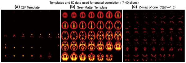
Grey matter and vCSF templates used for spatial correlation with the thresholded Z-map of the independent component.
2) Focusing degree defined by spatial entropy (S_enpy) and clustering degree (CD)
| (3) |
where i is the component index, both S_enpy and CD are normalized scalars in range of [0, 1].
Clustering degree is a measure of spatial structure (Formisano et al., 2002). For every IC, the number of voxels (Ntot) exceeding a threshold in the Z-map and the size of the subset of these voxels (Nclu) belonging to a 3D cluster of minimum extension (e.g. 3×3×3 voxel3) are computed. The CD is defined as CDi=Nclu/Ntot and is linearly scaled to be in the interval of [0, 1].
Spatial entropy is a measure of information content for one spatial distribution (De Martino et al., 2007), which is expected to be higher for component with more widely distributed values. We define
| (4) |
where hsi represents spatial histogram of the ith component computed over Nb bins. S_enpy is obtained by linear scaling of ∣ln (H)∣ so that it is in the range [0, 1].
Hence FD captures both the spatial distribution and the spatial structure information of one component. The movement-related artifact are shown as thin edge at the skull profile with opposite activated Z-values on two sides, such as top versus bottom or left versus right. The sparsely-distributed noises are by definition sparsely-distributed small activations. Both of them usually have fewer large-scale clustered activations or a wider spatial distribution than ICs of interest, so they are expected to have the lowest FD values. Suppose SFD is the sorted scalar FD from low to high, i.e., SFD(1) has the smallest value; MedFD is a measure defined by the median value of S_enpy and CD as follows, we use both MedFD and the sort order of FD to determine thFD dynamically:
| (5) |
| (6) |
where mth is the number of IC hypothesized as artifact. When FD<thFD, the IC is labeled as artifacts of such two types.
Demonstration of the artifact-removal method
Fig. 3 illustrated the most remarkable characteristics for 8 components decomposed from an fMRI dataset with a single Sternberg probe task. Our automated artifact removal method is applied to label every component and relies on two criteria: ‘CGM>CCSF’ and ‘FD>thFD’, whose values are binary with 0 (noise or artifacts) or 1 (non-artifact). As listed in the first two rows, if a component is labeled 0 for either of the criteria, it is classified as artifact or noise.
Fig. 3.
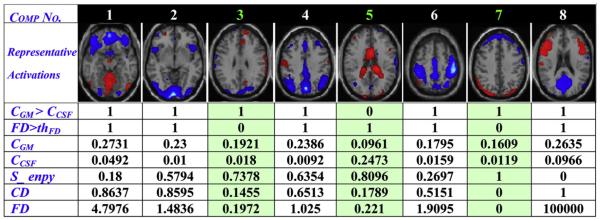
The most remarkable characteristics for 8 components decomposed from an fMRI dataset with a single Sternberg_probe task. Note that the 3rd IC is sparsely-distributed noise, the 5th IC is a vCSF artifact, the 7th IC manifests as movement-related artifact; and others appear to be ICs of interest. The descriptive measures used to classify the components are listed below in a table. All the 3 artifacts show zero (green background) in either of the criteria listed in the first two rows.
‘CGM>CCSF’
The correlation measures CGM and CCSF (listed in the 3rd and 4th row of Fig. 3) are used to label the vCSF artifact if ‘CGM>CCSF’ is false (value 0). For example, the 5th IC is marked as zero with CGM=0.0961<CCSF=0.2473 and Fig. 3 confirms that it is a vCSF artifact.
‘FD>thFD’
In case of Fig. 3, mth=8/4=2, SFD(2)=0.1972, SFD(4)=1.025 and MedFD=0.368; so thFD=SFD(2)=0.1972, then two ICs with the smallest FD values are labeled as artifact, i.e., the 3rd IC is sparsely-distributed noise and the 7th IC is movement-related artifact.
Optimal component/feature selection
For each of the 15 feature combinations, two non-artifact ICs (or one if duplicated) with the smallest p value or the largest J-divergence are selected out and termed “optimal components”. The two evaluation metrics are defined below:
p value, a measure which determines the probability of two groups having a significantly different mean in the mixing coefficients.
J-divergence (the symmetric Kullback–Leibler divergence), a measure reflecting the mutual information between the back-reconstructed source distributions of two groups (Calhoun et al., 2004a). The higher J-divergence value a component has, the larger difference exists between joint histogram distribution of Uh and Up.
Optimal feature selection
We define J-modulus, which is modulus of the J-divergences of two optimal components, as a measure of group-differentiating power of one feature combination. J modulus is ordered from high to low across all feature combinations to determine the optimal feature.
Optimal component selection
All non-artifact ICs of 15 combinations are sorted by J-divergence in descending order, several top ones are chosen as optimal components for all combinations.
Data sets
We used real fMRI data acquired at a single site, the Mind Research Network, collected as part of the MIND clinical imaging consortium, a large multisite fMRI study. Participants, including 25 schizophrenia patients and 28 healthy controls, had provided written, IRB-approved consent at University of New Mexico. They are scanned for all the following 3 tasks, which have been found to reveal robust activation differences in schizophrenia patients (Kumari et al., 2007; Manoach et al., 2001). The numbers of males/females are (23/5) and (22/3) for controls and patients respectively, and no significant group differences exist in age (controls, 32±13 years, range 18–54 years; patients, 32±12 years, range 21–60 years).
1) Auditory oddball task (target and novel)
The auditory oddball task stimulated the subject with three kinds of sounds: target (1200 Hz with probability, p=0.09), novel (computer generated complex tones, p=0.09), and standard (1000 Hz, p=0.82) presented through a computer system via sound insulated, MR-compatible earphones. Stimuli were presented sequentially in pseudorandom order for 200 ms each with inter-stimulus interval (ISI) varying randomly from 500 to 2050 ms. A subject was asked to make a quick button-press response with their right index finger upon each presentation of the target stimulus and no response was required for the other two stimuli. There were 4 runs, each comprising of 90 stimuli (3.2 min) (Kiehl and Liddle, 2001; Kiehl et al., 2005b).
2) Sternberg working memory task (encode and probe)
The Sternberg working memory task (Manoach et al., 1999, 2001) requires subjects to memorize a list of digits (displayed simultaneously) and later to identify if a ‘probe’ digit was in the list. Three working memory loads: high (5 digits), medium (3 digits) and low (1 digit) were used in this paradigm. Each run contained two blocks of each of the three loads in a pseudorandom order. Half of the probe digits were targets (digits previously displayed) and half were foils. Subjects were asked to respond with their right thumb if the probe digit was a target and with their left thumb for a foil.
3) Sensorimotor task
The sensorimotor task (Haslinger et al., 2005; Mattay et al., 1997) consisted of an on/off block design, each with a duration of 16s. During the on-block cycles of 8 ascending-pitched and 8 descending-pitched, 200 ms tones were presented. There were three runs each with duration of 4 min. The participant was instructed to press the right thumb of the input device after each tone was presented.
Imaging parameters
Scans were acquired at the Mind Research Network, on a 1.5 T dedicated head scanner (Siemens) with single echo planar imaging (EPI). The parameters for these functional scans are: TR = 2s, TE = 40 ms, FOV = 22 cm, acquisition matrix = 64 × 64, flip angle=90°, voxel size=3.75×3.75×4 mm, slice thickness=4 mm, gap=1 mm, 27 slices, AC-PC, Pulse sequence=PACE-enabled, single shot.
Image preprocessing
Data were preprocessed using the software package SPM5. Images were realigned using INRIalign, a motion correction algorithm unbiased by local signal changes (Freire et al., 2002). Data were spatially normalized into the standard MNI space (Friston et al., 1995), spatially smoothed with a 9 mm3 full width at half-maximum (FWHM) Gaussian kernel. The data, originally 3.75×3.75×4 mm, were slightly subsampled to 3×3×3 mm, resulting in 53×63×46 voxels.
GLM analysis
Data for each subject were analyzed by multiple regression with the SPM5 software. Regressors were created by modeling the predictors of interest as delta functions convolved with the default SPM5 hemodynamic response function (HRF). Contrast images were then calculated by applying appropriate linear contrasts to the parameter estimates for the parametric regressors of each task. After GLM analysis, the original fMRI 4D data of each subject is then reduced to be a 3D spatial map, i.e. “contrast image” or “feature”.
Results
Performance of the automated artifact removal method
The performance of the automated artifact removal method is evaluated when using different component number M. According to the minimum description length (MDL) principle (Li et al., 2007) and by applying it to multiple datasets, we find that for second-level fMRI analysis, M is usually in range of [8, 16], so 8, 12 and 16 components are chosen for data decomposition respectively. Every joint component contains 2 features, so there are (10×2+5)×M number of features that need to be classified. Only joint-ICs with both features shown as artifacts are automatically removed. If a joint component contains only one feature displayed as artifacts, it is still treated as an IC of interest, in order to keep potential useful information. The classification results from the proposed auto-artifact-removal method are compared with visual inspection results by experienced researchers and listed in Table 1, conditions in joint features (JF) and single feature (SF) are listed separately as JF/SF.
Table 1.
Results comparison of auto-artifact-removal method with visual inspection
| Number of ICs used | 8 | 12 | 16 | ||||
|
| |||||||
| Feature number classified | 160/40 | 240/60 | 320/80 | ||||
|
| |||||||
| Number of features(JF/SF) | Actual condition |
||||||
| Artifact | Non-artifact | Artifact | Non-artifact | Artifact | Non-artifact | ||
| Test shows “artifact” | 42/11 | 6/1 | 93/15 | 12/1 | 106/25 | 16/4 | |
| Test shows “non-artifact” | 9/0 | 103/28 | 14/3 | 121/41 | 10/4 | 188/47 | |
|
| |||||||
| False positive rate | 5.36%/3.57% | 8.89%/2.27% | 8.08%/7.84% | ||||
| Sensitivity | 82.35%/100% | 86.9%/83.3% | 91.38%/86.2% | ||||
| Accuracy of classification | 90.6%/97.5% | 89.2%/93.3% | 91.9%/90% | ||||
| Artifact ratio | 31.9%/27.5% | 44.6%/30% | 36.3%/36.3% | ||||
|
| |||||||
| Total false positive rate | 7.64%/4.88% | ||||||
| Total sensitivity | 87.96%/87.93% | ||||||
| Accuracy of classification | 90.7%/92.8% (average 91.1%) | ||||||
Note that our method performs robustly for different numbers of ICs. The error rates are computed as follows:
To avoid removing the components of interest, the false positive rate (FP) is controlled as 7.64% for all joint features and is lower than 5% (4.88%) for all single features. The true positive rates (sensitivity) show that nearly 88% of real artifacts are labeled correctly and the specificity (1-FP) for all features is 93%. Finally, the classification accuracy of our method is higher than 90% for all features and becomes quite efficient when analyzing large scale data, since it decreases the time needed for manual inspection.
In order to validate the effectiveness of our method to other datasets, we applied it to another dataset collected from a different scanner at the Olin Neuropsychiatry Research center in Hartford including 30 participants conducting the auditory oddball (target) task. The dataset was decomposed by CC-ICA using 8, 12 and 16 components respectively and labeled by the proposed method. The average classification accuracy is 91.7% compared to visual inspection. Hence, our automatic artifact removal method appears to generalize across different datasets.
Identified optimal features and components
Based on MDL with independent sampling (Li et al., 2007), 16 components are estimated from each of 10 joint feature combinations and 12 components are estimated from each of 5 single feature combinations, producing total 220 components consisting of 380 features.
For every feature combination, the J-modulus (right red bar) and the J-divergence of two optimal components based on the smallest p value (left blue bar) and the largest J-divergence (middle green bar) are illustrated in Fig. 4. Apparently, the SM single feature and the SBP&AODT joint feature are the top two combinations, so we pick them as two optimal features.
Fig. 4.

J-divergence of the optimal components selected by 2 criteria: the smallest p value (blue bar) and the largest J-divergence (green bar), for 15 feature combinations. The modulus of the above two J-divergence values are plotted as red bar, which is treated as the group discriminating power of each feature combination.
Fourteen components with J-divergence larger than 1.5 are plotted in Fig. 5 and their feature names are displayed on the bars. The top three components: SM7, SBP&AODT7 and SM6 stand out from others with J-divergence larger than 3. Hence they are regarded as the three optimal group-discriminating components and their spatial activations are investigated thoroughly in the next section.
Fig. 5.

Top 14 ICs with a J-divergence larger than 1.5 among all extracted ICs of 15 combinations. Their feature combination names are displayed on the bar. Component’s number of the top 3 ICs is also shown in bracket.
To verify the robustness of generating optimal features and components by the proposed framework, we changed the data by leaving ten controls and ten patients out and worked on a reduced dataset including 33 subjects. Results show the brain networks identified by the top 3 optimal components do not change, still, the top two optimal features are SM and SBP&AODT too. Thus, our framework derives consistent result in subset of the data on measuring group-differentiating capability.
Analysis of 3 optimal components
The three optimal components belong to two optimal feature combinations: SM and SBP&AODT. For display, the spatial maps of the 3 components are converted to Z-scores and thresholded at ∣Z∣>2.5 as shown in Fig. 6 (a), (b). Fig. 6 (c) gives a distinct view of the combined spatial maps in (a) and (b); these activated regions can best separate the two groups. The highlighted slices in (c) are back-reconstructed using Uh = Ah−1·Xh,Up = Ap−1·Xp and a significant group difference is indicated in (d) by subtracting patients from controls on their spatial maps, where controls have greater ∣Z∣ values is shown in orange and otherwise is shown in blue.
Fig. 6.

(a), (b) are the spatial maps of the top 3 optimal components, which are converted to Z-scores and thresholded at ∣Z∣>2.5; (c) shows the overlapping regions of the 4 features with their original spatial map values, these activated regions are important for group discrimination and may serve as biomarkers of schizophrenia patients; (d) displays the difference between the back-reconstructed sources (HC-SZ) on the combined highlighted regions of the top three optimal ICs in (c), the regions where HC>SZ in ∣Z∣ score are shown in orange, otherwise are shown in blue.
The thresholded Z maps of the 3 optimal components are converted to Talairach coordinates one by one, as listed in Table 2, and the most remarkable activated brain networks are interpreted.
Table 2.
Talairach table of the 3 optimal components
| Area | Brodmann area | R/L vol (cm3) | R/L max Z(x,y,z) |
|---|---|---|---|
| SM component 6 | |||
| Positive | |||
| Superior temporal gyrus | 22: 41 | 0.4/0.3 | 4.3(−50,14,−6)/4.1(59,−23,4) |
| Inferior/middle/medial frontal gyrus | 47: 45: 9: 6 | 0.7/0.1 | 3.9(−50,17,−6)/2.8(45,0,53) |
| Inferior parietal lobule | 40 | 0.3/0.0 | 3.5(−48,−41,55)/ns |
| Superior frontal gyrus | 6: 8 | 0.4/0.2 | 3.4(0,11,52)/3.1(3,6,60) |
| Insula | 13 | 0.3/0.0 | 3.0(−39,18,2)/ns |
| Negative | |||
| Posterior cingulate | 23: 31: 29: 30 | 0.9/0.8 | 6.2(−3,−51,22)/5.8(3,−51,22) |
| Precuneus | 31: 7: 19 | 1.6/1.8 | 5.5(0,−51,30)/5.1(3,−51,30) |
| Cingulate gyrus | 31 | 0.4/0.4 | 4.7(0,−45,30)/4.3(3,−45,30) |
| Cuneus | 7 | 0.2/0.2 | 4.6(0,−65,31)/4.3(3,−65,31) |
| Fusiform gyrus | 18 | 0.1/0.0 | 4.4(−27,−88,−16)/2.5(50,−53,−18) |
| Inferior parietal lobule | 39 | 0.0/1.0 | ns/4.2(45,−68,39) |
| Medial/middle/superior frontal gyrus | 10: 11 | 0.2/0.7 | 3.6(−3,62,16)/3.8(3,62,8) |
| Middle/superior temporal gyrus | 39:42 | 0.0/0.7 | ns/3.6(50,−66,23) |
| SM component 7 | |||
| Positive | |||
| Superior temporal gyrus | 42: 22: 41: 13 | 4.0/4.2 | 8.4(−62,−20,12)/7.4(50,−20,4) |
| Transverse temporal gyrus | 42: 41 | 0.9/1.1 | 7.7(−62,−17,12)/7.3(42,−31,13) |
| Middle temporal gyrus | 21: 22 | 1.2/0.7 | 6.9(−62,−6,−5)/5.0(59,−3,−5) |
| Insula | 13: 22: 41 | 0.3/1.2 | 6.1(−45,−17,4)/5.4(45,−17,4) |
| Postcentral gyrus | 43: 40: 1 | 0.1/0.0 | 3.2(−65,−19,20)/2.5(53,−18,45) |
| Inferior parietal lobule | 40 | 0.0/0.1 | ns/2.9(53,−46,22) |
| Lingual gyrus | 17 | 0.0/0.1 | ns/2.9(12,−94,−8) |
| Negative | |||
| Fusiform gyrus | 18 | 0.1/0.0 | 3.9(−27,−88,−16)/ns |
| SBP component 7 | |||
| Positive | |||
| Inferior/middle occipital gyrus | 17: 18 | 0.5/0.0 | 6.2(−24,−91,−8)/ns |
| Precentral gyrus | 6: 44 | 0.0/0.3 | ns/4.2(59,4,19) |
| Lingual gyrus | 17 | 0.1/0.0 | 4.0(−18,−94,−8)/ns |
| Inferior frontal gyrus | 44: 45 | 0.1/0.3 | 2.6(−42,38,9)/3.8(59,7,19) |
| Superior/middle/medial frontal gyrus | 11: 6 | 0.9/0.1 | 3.7(−30,40,−15)/ns |
| Cerebellum | 0.2/0.0 | 3.3(−36,−82,−16)/2.7(12,−82,−16) | |
| Cuneus | 17 | 0.3/0.0 | 3.3(−18,−96,0)/ns |
| Posterior cingulate | 31 | 0.0/0.1 | ns/2.8(9,−57,22) |
| Inferior parietal lobule | 40 | 0.1/0.0 | 2.8(−45,−59,47)/ns |
| Negative | |||
| Superior parietal lobule | 7 | 0.4/0.6 | 4.0(−30,−68,48)/4.5(33,−58,55) |
| Precuneus | 19: 7 | 0.8/0.5 | 4.3(−30,−77,40)/3.7(27,−80,40) |
| Superior frontal gyrus | 10: 8: 6 | 0.5/0.5 | 3.9(−3,17,52)/3.9(30,59,16) |
| Middle occipital gyrus | 18: 19 | 0.1/0.4 | 3.7(−50,−67,−9)/3.8(45,−76,−9) |
| Lingual gyrus | 18 | 0.0/0.4 | ns/3.7(18,−70,−9) |
| Middle/medial frontal gyrus | 10: 6: 8 | 0.1/0.1 | 3.2(−3,20,43)/3.3(30,62,8) |
| Cuneus | 19: 18 | 0.2/0.2 | 3.1(−3,−86,32)/3.2(15,−102,8) |
| Superior temporal gyrus | 22: 38 | 0.4/0.0 | 2.8(−56,11,−6)/ns |
| AODT component 7 | |||
| Positive | |||
| Cuneus | 17: 18: 19: 7 | 0.5/0.9 | 10.1(−3,−96,0)/8.9(3,−96,0) |
| Lingual gyrus | 17: 18 | 0.2/0.2 | 5.8(0,−90,−1)/6.1(6,−93,0) |
| Cerebellum | 0.4/0.1 | 3.4(−33,−56,−17)/2.7(27,−59,−17) | |
| Middle temporal gyrus | 21 | 0.3/0.0 | 3.3(−62,−18,−12)/ns |
| Superior temporal gyrus | 22 | 0.4/0.1 | 3.1(−65,−14,3)/3.0(53,14,−6) |
| Transverse temporal gyrus | 42 | 0.1/0.0 | 2.9(−65,−14,12)/ns |
| Fusiform gyrus | 19 | 0.1/0.0 | 2.8(−27,−56,−10)/ns |
| Postcentral gyrus | 2: 40 | 0.0/0.1 | ns/2.7(45,−29,54) |
| Middle occipital gyrus | 18 | 0.0/0.1 | ns/2.7(30,−96,0) |
| Negative | |||
| Inferior/middle occipital gyrus | 17: 18 | 0.6/0.1 | 6.1(−21,−94,−8)/3.0(27,−88,−8) |
| Lingual gyrus | 17 | 0.2/0.0 | 5.7(−18,−94,−8)/ns |
| Cerebellum | 0.2/0.1 | 2.6(−27,−34,−34)/4.5(6,−48,−33) | |
| Thalamus | 0.1/0.1 | 3.2(−3,−17,4)/3.7(3,−17,4) | |
| Posterior cingulate | 23: 29 | 0.1/0.1 | 2.8(−3,−55,14)/3.1(3,−52,14) |
| Superior/medial frontal gyrus | 6: 8 | 0.2/0.1 | 3.3(−3,20,60)/3.4(3,18,60) |
| Superior parietal lobule | 7 | 0.1/0.2 | 2.9(−21,−67,56)/2.8(24,−67,56) |
| Cuneus | 18 | 0.0/0.1 | ns/2.7(3,−72,15) |
| Precuneus | 7 | 0.0/0.1 | ns/2.7(24,−68,48) |
SM7: The temporal lobe network (Brodmann [BA] areas 21, 22, 38, 41, 42) which is associated with perception and recognition of auditory stimuli, memory, and speech, is identified as the most group-discriminative regions (Pearlson, 1997).
SBP&AODT7: The occipital lobe network including cuneus, lingual gyrus and occipital gyrus are identified in both features of this joint component.
SM6: A network which resembles the default mode network including precuneus, posterior cingulate, and BA 7, 10, and 39 (Correa et al., 2007) are identified as group-discriminating regions too. This component is derived from a second-level fMRI analysis, it is not really the same as, but looks very similar to the “default mode” derived from the first-level fMRI processing, so we will call it that in this paper. This brain network is proposed to participate in an organized, baseline default mode of brain function that is diminished during a variety of specific goal-directed behaviors (Raichle et al., 2001).
Further investigation of these highlighted regions including transverse and superior temporal gyrus, precuneus and posterior cingulated, cuneus and lingual gyrus, show that patients are more activated in ventral and medial superior temporal gyrus (STG) regions (including BA 38) and controls had greater activations in bilateral dorsal STG regions (which did not include BA 38). The default mode networks show negative Z-values for both groups, particularly, controls showed less activation in posterior cingulate than patients while had greater activation bilaterally on angular gyrus. In addition, a large region of cingulate gyrus and its surrounding sub-gyrus was activated in patients but not in controls. In addition, in occipital lobe, controls show stronger activations in cuneus (BA 18, 19) than SZ patients.
The optimal components are then utilized for the classification of patients and controls using a dataset collected from a different scanner. This dataset is also used to validate the auto-artifact-removal method and consists of 15 healthy controls and 15 schizophrenia patients. We generate five mask templates as listed in Table 3. Four of them based on the highlighted group-discriminative regions of the three optimal components as shown in Fig. 6 (c). Another mask is created by thresholding a two-sample t-test on the contrast images of the two reference groups at a significance level of p<0.0001, the regions of interest mainly occurred in temporal lobe and thalamus (now shown in the paper). The contrast image of every subject is masked via the template and the resulting nonzero voxels are transformed into a scalar with reduced dimension. We use mean of the absolute value of this scalar as the classifier input of each subject. Each individual was assigned one of two class memberships, with a leave-one-out approach based on the Euclidian distance between the individual and group means. Randomly selected subjects from each group were excluded from the whole data set, the classifier was designed using the remaining participants and tested on the two subjects. An average sensitivity and specificity were reported respectively in Table 3 for all masks. Note that the mask using combined regions generates the highest classification accuracy (sensitivity 87% and specificity 73%), while using the univariate method (t-test) results in a relatively lower accuracy (sensitivity 75% and specificity 64%). These results are quite encouraging considering the fact that the validation data was not only collected from different subjects, but also from a different MRI scanner.
Table 3.
Classification accurate using different masks with a leave-one-out method
| Mask | ‘Default mode’ (SM6) | Temporal lobe (SM7) | Lateral occipital lobe (SBP&AODT7) |
Combined three regions | Two sample t-test |
|---|---|---|---|---|---|
| Specificity | 0.52 | 0.60 | 0.70 | 0.73 | 0.64 |
| Sensitivity | 0.64 | 0.84 | 0.87 | 0.87 | 0.75 |
Analysis of two optimal feature combinations
For two optimal feature-combinations: SM and SBP&AODT, we were interested in investigating additional group-differentiating brain networks and exploring the potential associations which may be missed by separate analysis. To keep a balance for the contribution of the two combinations, the contrast images are concatenated as [SM,SM,SBP,AODT] with the same length of voxels for every feature and then stacked along subjects. 16 components are estimated via MDL criterion and decomposed by PCA-R+CC-ICA, the one with the largest J-divergence is thresholded by ∣Z∣>2.5 and is displayed in Fig. 7. Five main activated brain networks are demonstrated and converted to the Talairach coordinates. Table 4 lists the relevant Brodmann areas (both positive and negative) and their activated volumes.
Fig. 7.

The extracted joint component with the largest J-divergence from feature combination of [SM,SM,SBP,AODT]. The activations of the 3 features are transferred to Z score and thresholded at ∣Z∣>2.5.
Table 4.
Brodmann areas of the common brain networks identified across multi-features
| Brain networks | Features | SM |
SBP |
AODT |
|||
|---|---|---|---|---|---|---|---|
| Brodmann area | Vol (cm3) R/L | Brodmann area | Vol (cm3) R/L | Brodmann area | Vol (cm3) R/L | ||
| Temporal lobe: | Transverse/superior/middle temporal gyrus | 41,42,22,38,13 | 6.0/5.3 | 38 | 0.3/0.8 | 41,42, 22 | 0.9/1.7 |
| “Default mode”: | Precuneus, posterior cingulate etc. | NA | NA | 7,19,23,30,31,29 | 2.9/2.8 | 19,31,23,30,29,7 | 0.9/1.6 |
| Occipital lobe: | Lingual gyrus, cuneus,occipital gyrus | NA | NA | 7,18,19 | 0.7/0.9 | NA | NA |
| Parietal lobe: | Superior/inferior parietal lobule | NA | NA | 7,40 | 0.1/2.7 | 7,40 | 0.1/2.6 |
| Motor cortex: | Precentral gyrus, superior/medial frontal gyrus | 4,6,43,47 | 0.4/1.8 | 6,8,32 | 0.9/1.9 | 6,4,32,8 | 0.7/2.0 |
Discussion
For purposes of group discrimination and data fusion of large-scale fMRI data spanning multiple tasks, we proposed a novel framework that incorporates several key ideas: PCA-R, CC-ICA, automated artifact removal and optimal feature/component selection.
PCA-R is implemented in our initial data reduction step. The mean of group difference is adopted as a reference for measuring the discriminative power of the components, although other group information can also be introduced, this one is effective and computationally efficient (Chang, 1983), and selects out principal components with greatest potential to distinguish groups.
We proposed CC-ICA as an approach to incorporate prior group member information within the normal entropy cost function (for Infomax) to emphasize components that can best distinguish two groups. CC-ICA is designed to regularize the independence maximization by using a criterion which adaptively constrains specific mixing coefficients. Hence, the approach is not a strict constrained problem and the main role of λ is to regularize the solution. Optimization strategies are adopted to ensure the constraint enforces only when group differences really exist; otherwise, CC-ICA is identical to regular ICA. Our previous work (Sui et al., 2009) had shown CC-ICA can increase the estimation accuracy of both the components and the mixing coefficients compared to Infomax, and also brings about a change in the sorted order of the components, which may prove especially important in identifying optimal components. In this paper, we further extended its application to potential biomarker identification; considering the theme and the length of the paper, we didn’t show the results derived from Infomax.
In contrast to first-level ICA-based fMRI analysis methods, such as GIFT (Calhoun et al., 2001b), tensor probabilistic ICA (PICA) (Beckmann and Smith, 2005) and independent vector analysis (IVA) (Lee et al., 2008), CC-ICA is used for second-level fMRI analysis, it can work on either GLM contrast images (hypothesis-driven) or first-level ICA output maps (data-driven). We use GLM contrast images as input in this paper, as this is consistent with our previous work. It is straightforward to utilize components resulting from the first-level fMRI analysis in future work. Wang and Peterson (2008) also provides an option for selecting optimal first-level independent components as input (‘feature’) of our model. Further, by concatenating data from two modalities (e.g. functional MRI and structural MRI) instead of two fMRI-based features, CC-ICA can be extended to work with multi-modal data analysis, hence it has wide applicability in neuroimaging field.
We propose a novel automated artifact removal method for components derived from second-level fMRI analysis, which effectively accelerates the components’ classification especially when hundreds of ICs need to be analyzed. This method is designed to automatically remove the artifacts with obvious noise characteristics, rather than all “possible artifact” components, such as the component displaying both meaningful activations and vCSF artifact. We leave these noise-mixed components for further visual inspection. Since no time-domain information is available for components extracted from feature-based ICA, our method only depends on general spatial measures. Though it is possible to include other measures to improve the classification accuracy, our method is very straightforward and efficiently attains high sensitivity (88%) and a low false positive rate (7%). Application to a separate dataset also validates its generalizability.
The first criterion is based on the spatial correlation with vCSF and GM template, which can remove vCSF artifact effectively while simultaneously keeping noise-mixed components if their activations in GM are stronger than those in vCSF. Using spatial mask to remove the data in vCSF region before we starting analysis is also an option, but after smoothing, the voxels in vCSF region may contain GM information, in order to keep useful information as much as possible and retain the integrality of raw data, we chose the former option. The only parameter that is user selected in our artifact selection approach is the Z-score value. Our experience working with many data sets suggests that a value ∣Z∣>1.5 is a good choice and provides reliable performance. Also, we noted the robustness of the method to variations of Z-score when it is chosen around this value.
The three optimal components we identified suggest that aberrant patterns in temporal lobe, default mode and occipital lobe are shown in schizophrenia, which is consistent with previous findings. Specifically, first, various studies have shown that superior temporal gyrus is significantly different in schizophrenia (Pearlson, 1997) and one of the most robust functional abnormalities in schizophrenia manifests as a decrease in the temporal lobe amplitude of the oddball response in both event-related potential (ERP) data (McCarley et al., 1991) and fMRI data (Kiehl and Liddle, 2001). The bilateral temporal lobe has also been used for successful discrimination of HC and SZ (Calhoun et al., 2004b). Second, in task-related fMRI studies, activity deficits in the occipital cortex had been observed in schizophrenic patients compared with controls (Johnston et al., 2005; Tregellas et al., 2004), and there were evidences supporting that the activity of the occipital lobe is abnormal in schizophrenia in both resting-state (Liu et al., 2006) and non-task-related fMRI studies such as AOD task (Kiehl et al., 2005a). This region may perhaps be differentially activated because the Sternberg task has a visual component. Finally, schizophrenia is found associated with altered temporal frequency and spatial location of the default mode network (Bluhm et al., 2007; Garrity et al., 2007).
Note that each of these brain networks was identified separately in previous neuroimaging studies (Garrity et al., 2007; Kiehl et al., 2005a; Tregellas et al., 2004), however our approach grouped them together in a framework that specifically identifies group discriminative features. Such a result is not obtainable using traditional approaches which focus upon a single task. Moreover, the optimal components may only be ‘identifiable’ through stimulation and comparison by different tasks, which further motivates a data fusion approach.
Initial classification results on a novel dataset indicate that combining information from all optimal components provides an encouraging classification accuracy (sensitivity 87% and specificity 73%) and an improved ability to classify memberships compared with each approach individually, see Table 3. Compared with clinical symptoms, which typically need to be combined with outcome data tracked over a period of months in order to develop an accurate diagnosis, the group-differentiating brain networks derived by our framework are less variable and may also be useful for classification, see Calhoun et al. (2008), however a full examination of the classification potential is beyond the scope of our current work. These initial results suggest our method can generate optimal components which may have great potential to serve as biomarkers for certain brain disorders.
We focus on between-group differences (no within-group differences) in this paper. The weakness of the univariate methods on joint analysis (e.g., regression analysis, t-test, ANOVA) lies in that they cannot identify covariation patterns of the same subject, thus wouldn’t enable us to identify joint information. In addition, the artifacts and effective brain activations are all mixed together when using univariate methods, so the artifactual signals will not be separated from signals of interest; while this can be solved readily by ICA-based methods. The initial classification results also prove the advantage of our method over a univariate method.
Another point we should keep in mind is that it is not sufficient to only identify the optimal regions, to identify the tasks within which these circuits are engaged is also significant. This is the strength of our approach. By analyzing multiple fMRI tasks, the selection of features for group discrimination/classification is proved to be crucial. SM is suggested the best group-differentiating feature; its 3 ICs occur in top 4 ones with the largest J-divergence. This optimal feature shows several brain modes that demonstrate robust functional disturbances in schizophrenia patients (Hazlett and Buchsbaum, 2001; Mattay et al., 1997), such as temporal lobe and default mode circuits. The sensorimotor task was also found to best discriminate schizophrenia from control subjects in a classification approach comparing the same three tasks (Demirci et al., 2008). In addition to SM, we found that a joint feature SBP&AODT is the second most group-discriminative feature.
To explore whether additional benefit could be obtained, we also performed a 4-way joint ICA analysis ([SM SM SBP AODT]) on two optimal feature: SM and SBP&AODT. It is notable that identified brain networks in Fig. 7 are largely similar to those indicated in Fig. 6(c). Specifically, temporal lobe still contains the most prominent activated regions in the SM feature and contains voxels with the largest Z-value among all 3 features; a network which resembles the default mode now shows up in SBP&AODT (previously in the SM feature); the occipital regions involved in pattern recognition and visual attention are identified in the SBP features. Note that all three features also include regions in primary and secondary motor cortex (BA 4, 6), accompanied by a functional asymmetry with left dominance, consistent with the fact that all the three tasks need participants push the button with their right fingers. Except the four common regions to those displayed in Fig. 6 (c), additional activations in parietal lobe with left dominance show up in the SBP&AODT feature but not in the SM feature. Parietal lobe is involved in multiple functions including attention, visuospatial abilities, sensory integration (Andersen and Buneo, 2002; Bendiksby and Platt, 2006) and decision making (McClure et al., 2004). Our finding is consistent with the fact that both the Sternberg and AOD tasks require signal discrimination (i.e., target vs. novel in AOD, digits previously displayed or not in SB), but there is no such requirement in the SM task. Therefore the multi-way (more than 2) joint CC-ICA results appears to identify more inter-task relationships, while it generates similar conclusions to the 2-way joint CC-ICA on identifying the most group-discriminative regions.
In order to identify the best group differentiating aspect we proposed the J modulus, which incorporates information from both mixing coefficients and the estimated sources. Although other criterions may also be applicable, our measure is straightforward and generates reasonable results on optimal feature selection.
We have also shown our framework derives consistent results from a different data subset, which demonstrates that the optimal selection results are not biased toward a particular dataset and are hence more likely to be reproducible.
Investigating schizophrenia-related deficits in functional connectivity among the optimal components we identified here will be an important future goal, since previous studies show evidence that schizophrenia involves a defect in the functional integrity of neural circuits or dysfunctional connectivity in multiple brain regions including temporal lobe (Friston and Frith, 1995; Kiehl et al., 2005a) and default mode (Garrity et al., 2007; Zhou et al., 2007). This work may provide a template for differential diagnosis of multiple brain disorders.
We also hope to further validate the results in future studies using a split-half resampling technique under the NPAIRS framework (Nonparametric Prediction, Activation, Influence and Reproducibility reSampling) (Strother et al., 2002). This technique provides a way to compare differences between two groups and among participants in the same group. It may also be useful to incorporate other prior information or different distributions for different features into the model. Application to data in other modalities such as EEG can also be implemented to investigate the significant group differences.
In conclusion, we proposed a novel framework for selection of group discriminating aspects from multiple fMRI tasks. An automated artifact removal method with an accuracy of 91% is also proposed to accelerate optimal component selection. Application of our method to a schizophrenia dataset shows that SM and SBP&AODT are two optimal features. Also, three optimal components including brain networks of temporal lobe, default mode and occipital lobe are suggested to be most sensitive in distinguishing schizophrenia from controls and show great promise as potential illness markers.
Acknowledgments
This work was supported by the National Institutes of Health grants 1 R01 EB 006841 and 1 R01 EB 005846 (to Vince D. Calhoun) and MH43775, MH074797 and MH077945 (to Godfrey D. Pearlson). We thank the research staff at the University of New Mexico and the Mind Research Network who helped collect and process the data. We also appreciate the valuable advice given by the members of the Medical Image Analysis Laboratory, especially Jingyu Liu, Rogers Ferreira da Silva, Lei Wu and Lai Xu at the Mind Research Network.
Appendix.
PCA-R
Principal components analysis is a typically used preprocessing step in multivariate data analysis to decompose data into a set of uncorrelated principal components ordered by the variance of each component. Suppose there are nh healthy controls and np patients, nh+np=N, the observed data X consists of measurements from all subjects with dimensions of N×L (subjects by voxels). In a typical use of PCA for dimensionality reduction, assume Λ and B are, respectively, the diagonal eigenvalue and eigenvector matrix of the covariance matrix E{X·XT}, Λ=diag{λ1, λ2…λN}. The top M components (M<N) with the largest λi are selected, thus Λ is changed to Λ’, an M×M diagonal matrix, and B is reduced to an corresponding M×N matrix B’. Therefore the reduced data X’ is given by X’=Λ’−1/2·B’·X.
In PCA-R, a categorical variable such as the mean group difference, is incorporated as a reference r for measuring a component’s discriminate power φi. We define
| (A.1) |
| (A.2) |
where bi is the ith column of matrix B. After sorting φi in a descending order, as well as the corresponding eigenvectors, the top M components are selected for discriminative purpose by projecting X into the top M eigenvectors and X’ can be obtained in a similar way. Assume X’=D·X, the M×N matrix D is called whitening matrix and is used for dimension reconstruction of mixing matrix A during CC-ICA optimization.
CC-ICA
To account for group inferences, the regular ICA model can be extended as
| (A.3) |
Ah,Ap are mixing matrices in dimension of nh×M and np×M, each column of which represents loading parameters for one shared component. For the ith component, i=1,2…M, assume scalar Ah,i,Ap,i (the ith column of matrix Ah,Ap) are its corresponding subject-specific loading parameters for two groups. The mean of Ah,i and Ap,i represent the contribution of the ith component to different groups. The T statistic to test whether their means are different can be calculated as follows:
| (A.4) |
where the symbol and and Sh,i(Sp,i) are the mean and the standard derivation of Ah,i(Ap,i). nh +np−2 is the number of degrees of freedom for two-tailed significance testing. The larger the absolute value of Ti, the higher the probability that the mixing coefficients’ averages of the ith component are significantly different for two groups.
The cost function C of CC-ICA is constructed as:
| (A.5) |
| (A.6) |
| (A.7) |
where u and y are the nonlinear network input and output scalar. The nonlinear sigmoid function g(·) has been shown to be quite robust to violations of the underlying model for a wide variety of data types. Here, E{·} is the expectation operator, H{·} is the differential entropy of y, λ represents the constraint strength and suffix i refers to the index of the constrained component(s).
The main purpose of CC-ICA is to estimate the unmixing matrix W by maximizing C. The learning process is as follows: for a selected iterative ICA algorithm, we assume the unmixing matrix obtained at the kth iteration is Wk,sICA, thus Wk,sICA will iteratively converge with the maximization of H. In case of Infomax, Wk,sICA is updated by the natural gradient learning rule (Amari, 1998) as
| (A.8) |
Only when weight change ΔWk,sICA stabilizes (measured by a tolerance factor), the constraint takes effect, namely λ>0; now Ah and Ap are determined by , D is the whitening matrix defined in PCA-R. is then maximized by the steepest ascent learning rule using partial derivatives of Ah,i and Ap,i, as shown in (A.9,10), i denotes the column index of the constrained components.
| (A.9) |
| (A.10) |
After updating Ah and Ap, Wk is obtained according to (A.11).
| (A.11) |
In the next iteration, Wk is then updated to Wk + 1,sICA according to Eq. (A.8). The learning process is repeated until convergence of Wk achieved, which is to some degree similar to that used in set-membership normalized least mean square (SM-NLMS) algorithm (Gollamudi et al., 1998).
Note that which components are constrained is not fixed; rather, they are allowed to vary during the optimization. After constraint takes effect, T2 values of all components are calculated as Eq. (A.4) and are sorted at the current and the following steps. Half or more number of components with the highest T2 values are selected to be constrained to ensure that all components which may capture group differences are potentially constrained.
To ensure CC-ICA to adaptively adjust the learning process with the dataset, two optimization strategies are adopted:
We adaptively adjust the constraint strength λ. Specifically, after the constrained components are determined, the constraint is incorporated with a strength λ0 (initial learning rate). λ0 is estimated by a testing loop so that the absolute correlation value between Wk,sICA and Wk (the weight matrix obtained before and after adding the constraint) is bigger than 0.99. Furthermore, to achieve mutual independence between the components, the slope of ΔWk during the last ten steps SlopeΔW,10 is used to supervise the learning process so that the entropy maximization dominates the Wk update process. λ0 is scaled down by 0.9 when SlopeΔW,10>0.
We put an adaptive stopping rule in place which enables CC-ICA to converge to regular ICA if no group differences exist. When there are few or no components with a true group difference, the SlopeΔW,10 can also act as a switch for the constraint. In this case, entropy will fall suddenly and consequently ΔWk will increase abruptly, so when SlopeΔW,10 exceeds the threshold thstop (e.g., thstop=0.001), λ is set to be zero and the learning process converges to regular ICA. Hence the supervision by SlopeΔW,10 prevents the constraint from producing spurious group differences.
References
- Adali T, Li H, Novey M, Cardoso JF. Complex ICA using nonlinear functions. IEEE Trans. Signal Process. 2008;56(9):4536–4544. [Google Scholar]
- Amari S. Natural gradient works efficiently in learning. Neural Comput. 1998;10:251–276. [Google Scholar]
- Andersen RA, Buneo CA. Intentional maps in posterior parietal cortex. Annu. Rev. Neurosci. 2002;25:189–220. doi: 10.1146/annurev.neuro.25.112701.142922. [DOI] [PubMed] [Google Scholar]
- Beckmann CF, Smith SM. Tensorial extensions of independent component analysis for multisubject FMRI analysis. NeuroImage. 2005;25(1):294–311. doi: 10.1016/j.neuroimage.2004.10.043. [DOI] [PubMed] [Google Scholar]
- Bell AJ, Sejnowski TJ. An information-maximization approach to blind separation and blind deconvolution. Neural Comput. 1995;7(6):1129–1159. doi: 10.1162/neco.1995.7.6.1129. [DOI] [PubMed] [Google Scholar]
- Bendiksby MS, Platt ML. Neural correlates of reward and attention in macaque area LIP. Neuropsychologia. 2006;44(12):2411–2420. doi: 10.1016/j.neuropsychologia.2006.04.011. [DOI] [PubMed] [Google Scholar]
- Bluhm RL, Miller J, Lanius RA, Osuch EA, Boksman K, Neufeld RW, Theberge J, Schaefer B, Williamson P. Spontaneous low-frequency fluctuations in the BOLD signal in schizophrenic patients: anomalies in the default network. Schizophr. Bull. 2007;33(4):1004–1012. doi: 10.1093/schbul/sbm052. [DOI] [PMC free article] [PubMed] [Google Scholar]
- Calhoun VD, Adali T, McGinty VB, Pekar JJ, Watson TD, Pearlson GD. fMRI activation in a visual-perception task: network of areas detected using the general linear model and independent components analysis. NeuroImage. 2001a;14(5):1080–1088. doi: 10.1006/nimg.2001.0921. [DOI] [PubMed] [Google Scholar]
- Calhoun VD, Adali T, Pearlson GD, Pekar JJ. A method for making group inferences from functional MRI data using independent component analysis. Hum. Brain Mapp. 2001b;14(3):140–151. doi: 10.1002/hbm.1048. [DOI] [PMC free article] [PubMed] [Google Scholar]
- Calhoun VD, Adali T, Pearlson GD, Pekar JJ. Spatial and temporal independent component analysis of functional MRI data containing a pair of task-related waveforms. Hum. Brain Mapp. 2001c;13(1):43–53. doi: 10.1002/hbm.1024. [DOI] [PMC free article] [PubMed] [Google Scholar]
- Calhoun VD, Adali T, Pekar JJ. A method for comparing group fMRI data using independent component analysis: application to visual, motor and visuomotor tasks. Magn. Reson. Imaging. 2004a;22(9):1181–1191. doi: 10.1016/j.mri.2004.09.004. [DOI] [PubMed] [Google Scholar]
- Calhoun VD, Kiehl KA, Liddle PF, Pearlson GD. Aberrant localization of synchronous hemodynamic activity in auditory cortex reliably characterizes schizophrenia. Biol. Psychiatry. 2004b;55(8):842–849. doi: 10.1016/j.biopsych.2004.01.011. [DOI] [PMC free article] [PubMed] [Google Scholar]
- Calhoun VD, Adali T, Giuliani NR, Pekar JJ, Kiehl KA, Pearlson GD. Method for multimodal analysis of independent source differences in schizophrenia: combining gray matter structural and auditory oddball functional data. Hum. Brain Mapp. 2006a;27(1):47–62. doi: 10.1002/hbm.20166. [DOI] [PMC free article] [PubMed] [Google Scholar]
- Calhoun VD, Adali T, Kiehl KA, Astur R, Pekar JJ, Pearlson GD. A method for multitask fMRI data fusion applied to schizophrenia. Hum. Brain Mapp. 2006b;27(7):598–610. doi: 10.1002/hbm.20204. [DOI] [PMC free article] [PubMed] [Google Scholar]
- Calhoun VD, Maciejewski PK, Pearlson GD, Kiehl KA. Temporal lobe and “default” hemodynamic brain modes discriminate between schizophrenia and bipolar disorder. Hum. Brain Mapp. 2008;29(11):1265–1275. doi: 10.1002/hbm.20463. [DOI] [PMC free article] [PubMed] [Google Scholar]
- Calhoun VD, Silva R, Liu J. Identification Of Multimodal MRI and EEG Biomarkers Using Joint-ICA and Divergence Criteria. Thessaloniki; Greece: Aug, 2007. [Google Scholar]
- Caprihan A, Pearlson GD, Calhoun VD. Application of principal component analysis to distinguish patients with schizophrenia from healthy controls based on fractional anisotropy measurements. Neuroimage. 2008;42(2):675–682. doi: 10.1016/j.neuroimage.2008.04.255. [DOI] [PMC free article] [PubMed] [Google Scholar]
- Cardoso JF. Infomax and maximum likelihood for source separation. IEEE Lett. Signal Process. 1997;4(4):112–114. [Google Scholar]
- Chang WC. On using principle components before separating a mixture of two multivariate normal distributions. Appl. Stat. 1983;32:267–275. [Google Scholar]
- Choi K, Yang Z, Hu X, Mayberg H. A Combined Functional–Structural Connectivity Analysis of Major Depression Using Joint Independent Components Analysis. Psychiatric MRI/MRS; Toronto,Cananda: May 3–9, 2008. p. 3555. [Google Scholar]
- Correa N, Adali T, Calhoun VD. Performance of blind source separation algorithms for fMRI analysis using a group ICA method. Magn. Reson. Imaging. 2007;25(5):684–694. doi: 10.1016/j.mri.2006.10.017. [DOI] [PMC free article] [PubMed] [Google Scholar]
- De Martino F, Gentile F, Esposito F, Balsi M, Di Salle F, Goebel R, Formisano E. Classification of fMRI independent components using IC-fingerprints and support vector machine classifiers. NeuroImage. 2007;34(1):177–194. doi: 10.1016/j.neuroimage.2006.08.041. [DOI] [PubMed] [Google Scholar]
- Demirci O, Clark VP, Magnotta VA, Andreasen NC, Lauriello J, Kiehl KA, Pearlson GD, Calhoun DC. A review of challenges in the use of fMRI for disease classification/characterization and a projection pursuit application from multi-site fMRI schizophrenia study. Brain Imaging and Behavior. 2008;2(3):207–226. doi: 10.1007/s11682-008-9028-1. [DOI] [PMC free article] [PubMed] [Google Scholar]
- Dillon RW, Mulani N, Frederick GD. On the use of component scores in the presence of group structure. J. Consum. Res. 1989;16:106–112. [Google Scholar]
- Esposito F, Scarabino T, Hyvarinen A, Himberg J, Formisano E, Comani S, Tedeschi G, Goebel R, Seifritz E, Di Salle F. Independent component analysis of fMRI group studies by self-organizing clustering. NeuroImage. 2005;25(1):193–205. doi: 10.1016/j.neuroimage.2004.10.042. [DOI] [PubMed] [Google Scholar]
- Formisano E, Esposito F, Kriegeskorte N, Tedeschi G, Di Salle F, Goebel R. Spatial independent component anaysis of functional magnetic resonance imaging time series: characterization of the cortical components. Neural Comput. 2002;49(1–4):241–254. [Google Scholar]
- Freire L, Roche A, Mangin JF. What is the best similarity measure for motion correction in fMRI time series? IEEE Trans. Med. Imag. 2002;21(5):470–484. doi: 10.1109/TMI.2002.1009383. [DOI] [PubMed] [Google Scholar]
- Friston KJ, Frith CD. Schizophrenia: a disconnection syndrome? Clin. Neurosci. 1995;3(2):89–97. [PubMed] [Google Scholar]
- Friston KJ, Ashburner J, Frith CD, Poline JP, Heather JD, Frackowiak RS. Spatial registration and normalization of images. Hum. Brain Mapp. 1995;2:165–189. [Google Scholar]
- Garrity AG, Pearlson GD, McKiernan K, Lloyd D, Kiehl KA, Calhoun VD. Aberrant “default mode” functional connectivity in schizophrenia. Am. J. Psychiatry. 2007;164(3):450–457. doi: 10.1176/ajp.2007.164.3.450. [DOI] [PubMed] [Google Scholar]
- Gollamudi S, Nagaraj S, kapoor S, Huang YH. Set-membership filtering and a set-membership normalized LMS algorithm with an adaptive step size. IEEE Signal Process. Lett. 1998;5(5):111–114. [Google Scholar]
- Grady CL, Springer MV, Hongwanishkul D, McIntosh AR, Winocur G. Age-related changes in brain activity across the adult lifespan. J. Cogn. Neurosci. 2006;18(2):227–241. doi: 10.1162/089892906775783705. [DOI] [PubMed] [Google Scholar]
- Guo Y, Pagnoni G. A unified framework for group independent component analysis for multi-subject fMRI data. NeuroImage. 2008;42(3):1078–1093. doi: 10.1016/j.neuroimage.2008.05.008. [DOI] [PMC free article] [PubMed] [Google Scholar]
- Haslinger B, Erhard P, Altenmuller E, Schroeder U, Boecker H, Ceballos-Baumann AO. Transmodal sensorimotor networks during action observation in professional pianists. J. Cogn. Neurosci. 2005;17(2):282–293. doi: 10.1162/0898929053124893. [DOI] [PubMed] [Google Scholar]
- Hazlett EA, Buchsbaum MS. Sensorimotor gating deficits and hypofrontality in schizophrenia. Front. Biosci. 2001;6:D1069–D1072. doi: 10.2741/hazlett. [DOI] [PubMed] [Google Scholar]
- Hesse CW, James CJ. On semi-blind source separation using spatial constraints with applications in EEG analysis. IEEE Trans. Biomed. Eng. 2006;53(12 Pt 1):2525–2534. doi: 10.1109/TBME.2006.883796. [DOI] [PubMed] [Google Scholar]
- Johnson MR, Morris NA, Astur RS, Calhoun VD, Mathalon DH, Kiehl KA, Pearlson GD. A functional magnetic resonance imaging study of working memory abnormalities in schizophrenia. Biol. Psychiatry. 2006;60(1):11–21. doi: 10.1016/j.biopsych.2005.11.012. [DOI] [PubMed] [Google Scholar]
- Johnston PJ, Stojanov W, Devir H, Schall U. Functional MRI of facial emotion recognition deficits in schizophrenia and their electrophysiological correlates. Eur. J. Neurosci. 2005;22(5):1221–1232. doi: 10.1111/j.1460-9568.2005.04294.x. [DOI] [PubMed] [Google Scholar]
- Jolliffe IT, Morgan BJ, Young PJ. A simulation study of the use of principle component in linear discriminant analysis. J. Stat. Comput. Simul. 1996;55:353–366. [Google Scholar]
- Kiehl KA, Liddle PF. An event-related functional magnetic resonance imaging study of an auditory oddball task in schizophrenia. Schizophr. Res. 2001;48(2–3):159–171. doi: 10.1016/s0920-9964(00)00117-1. [DOI] [PubMed] [Google Scholar]
- Kiehl KA, Stevens MC, Celone K, Kurtz M, Krystal JH. Abnormal hemodynamics in schizophrenia during an auditory oddball task. Biol. Psychiatry. 2005a;57(9):1029–1040. doi: 10.1016/j.biopsych.2005.01.035. [DOI] [PMC free article] [PubMed] [Google Scholar]
- Kiehl KA, Stevens MC, Laurens KR, Pearlson G, Calhoun VD, Liddle PF. An adaptive reflexive processing model of neurocognitive function: supporting evidence from a large scale (n=100) fMRI study of an auditory oddball task. NeuroImage. 2005b;25(3):899–915. doi: 10.1016/j.neuroimage.2004.12.035. [DOI] [PubMed] [Google Scholar]
- Kochiyama T, Morita T, Okada T, Yonekura Y, Matsumura M, Sadato N. Removing the effects of task-related motion using independent-component analysis. NeuroImage. 2005;25(3):802–814. doi: 10.1016/j.neuroimage.2004.12.027. [DOI] [PubMed] [Google Scholar]
- Kumari V, Antonova E, Geyer MA, Ffytche D, Williams SC, Sharma T. A fMRI investigation of startle gating deficits in schizophrenia patients treated with typical or atypical antipsychotics. Int. J. Neuropsychopharmacol. 2007;10(4):463–477. doi: 10.1017/S1461145706007139. [DOI] [PubMed] [Google Scholar]
- Lee JH, Lee TW, Jolesz FA, Yoo SS. Independent vector analysis (IVA): multivariate approach for fMRI group study. NeuroImage. 2008;40(1):86–109. doi: 10.1016/j.neuroimage.2007.11.019. [DOI] [PubMed] [Google Scholar]
- Li YO, Adali T, Calhoun VD. Estimating the number of independent components for functional magnetic resonance imaging data. Hum. Brain Mapp. 2007;28(11):1251–1266. doi: 10.1002/hbm.20359. [DOI] [PMC free article] [PubMed] [Google Scholar]
- Liddle PF, Friston KJ, Frith CD, Hirsch SR, Jones T, Frackowiak RS. Patterns of cerebral blood flow in schizophrenia. Br. J. Psychiatry. 1992;160:179–186. doi: 10.1192/bjp.160.2.179. [DOI] [PubMed] [Google Scholar]
- Lin FH, McIntosh AR, Agnew JA, Eden GF, Zeffiro TA, Belliveau JW. Multivariate analysis of neuronal interactions in the generalized partial least squares framework: simulations and empirical studies. NeuroImage. 2003;20(2):625–642. doi: 10.1016/S1053-8119(03)00333-1. [DOI] [PubMed] [Google Scholar]
- Liu H, Liu Z, Liang M, Hao Y, Tan L, Kuang F, Yi Y, Xu L, Jiang T. Decreased regional homogeneity in schizophrenia: a resting state functional magnetic resonance imaging study. NeuroReport. 2006;17(1):19–22. doi: 10.1097/01.wnr.0000195666.22714.35. [DOI] [PubMed] [Google Scholar]
- Liu J, Xu L, Calhoun VD. Extracting principle components for discriminant analysis of fMRI images. IEEE; Las Vegas, USA: Mar 30 4, Apr 30 4, 2008. pp. 449–452. [DOI] [PMC free article] [PubMed] [Google Scholar]
- Liu J, Pearlson GD, Windemuth A, Ruano G, Perrone-Bizzozero NI, Calhoun VD. Combining fMRI and SNP data to investigate connections between brain function and genetics using parallel ICA. Hum. Brain Mapp. 2009;30(1):241–255. doi: 10.1002/hbm.20508. [DOI] [PMC free article] [PubMed] [Google Scholar]
- Lu W, Rajapakse JC. Approach and applications of constrained ICA. IEEE Trans. Neural Netw. 2005;16(1):203–212. doi: 10.1109/TNN.2004.836795. [DOI] [PubMed] [Google Scholar]
- Lu WaR JC. ICA with reference. Neural Comput. 2004;69(16–18):2244–2257. [Google Scholar]
- Manoach DS, Press DZ, Thangaraj V, Searl MM, Goff DC, Halpern E, Saper CB, Warach S. Schizophrenic subjects activate dorsolateral prefrontal cortex during a working memory task, as measured by fMRI. Biol. Psychiatry. 1999;45(9):1128–1137. doi: 10.1016/s0006-3223(98)00318-7. [DOI] [PubMed] [Google Scholar]
- Manoach DS, Halpern EF, Kramer TS, Chang Y, Goff DC, Rauch SL, Kennedy DN, Gollub RL. Test–retest reliability of a functional MRI working memory paradigm in normal and schizophrenic subjects. Am. J. Psychiatry. 2001;158(6):955–958. doi: 10.1176/appi.ajp.158.6.955. [DOI] [PubMed] [Google Scholar]
- Mattay VS, Callicott JH, Bertolino A, Santha AK, Tallent KA, Goldberg TE, Frank JA, Weinberger DR. Abnormal functional lateralization of the sensorimotor cortex in patients with schizophrenia. NeuroReport. 1997;8(13):2977–2984. doi: 10.1097/00001756-199709080-00034. [DOI] [PubMed] [Google Scholar]
- McCarley RW, Faux SF, Shenton ME, Nestor PG, Adams J. Event-related potentials in schizophrenia: their biological and clinical correlates and a new model of schizophrenic pathophysiology. Schizophr. Res. 1991;4(2):209–231. doi: 10.1016/0920-9964(91)90034-o. [DOI] [PubMed] [Google Scholar]
- McClure SM, Laibson DI, Loewenstein G, Cohen JD. Separate neural systems value immediate and delayed monetary rewards. Science. 2004;306(5695):503–507. doi: 10.1126/science.1100907. [DOI] [PubMed] [Google Scholar]
- McIntosh AR, Bookstein FL, Haxby JV, Grady CL. Spatial pattern analysis of functional brain images using partial least squares. NeuroImage. 1996;3(3 Pt 1):143–157. doi: 10.1006/nimg.1996.0016. [DOI] [PubMed] [Google Scholar]
- McKeown MJ. Detection of consistently task-related activations in fMRI data with hybrid independent component analysis. NeuroImage. 2000;11(1):24–35. doi: 10.1006/nimg.1999.0518. [DOI] [PubMed] [Google Scholar]
- McKeown MJ, Makeig S, Brown GG, Jung TP, Kindermann SS, Bell AJ, Sejnowski TJ. Analysis of fMRI data by blind separation into independent spatial components. Hum. Brain Mapp. 1998;6(3):160–188. doi: 10.1002/(SICI)1097-0193(1998)6:3<160::AID-HBM5>3.0.CO;2-1. [DOI] [PMC free article] [PubMed] [Google Scholar]
- McKeown MJ, Hansen LK, Sejnowsk TJ. Independent component analysis of functional MRI: what is signal and what is noise? Curr. Opin. Neurobiol. 2003;13(5):620–629. doi: 10.1016/j.conb.2003.09.012. [DOI] [PMC free article] [PubMed] [Google Scholar]
- McKeown MJ, Li J, Huang X, Lewis MM, Rhee S, Young Truong KN, Wang ZJ. Local linear discriminant analysis (LLDA) for group and region of interest (ROI)-based fMRI analysis. NeuroImage. 2007;37(3):855–865. doi: 10.1016/j.neuroimage.2007.04.072. [DOI] [PubMed] [Google Scholar]
- Pearlson GD. Superior temporal gyrus and planum temporale in schizophrenia: a selective review. Prog. Neuro-psychopharmacol. Biol. Psychiatry. 1997;21(8):1203–1229. doi: 10.1016/s0278-5846(97)00159-0. [DOI] [PubMed] [Google Scholar]
- Perlbarg V, Bellec P, Anton JL, Pelegrini-Issac M, Doyon J, Benali H. CORSICA: correction of structured noise in fMRI by automatic identification of ICA components. Magn. Reson. Imaging. 2007;25(1):35–46. doi: 10.1016/j.mri.2006.09.042. [DOI] [PubMed] [Google Scholar]
- Raichle ME, MacLeod AM, Snyder AZ, Powers WJ, Gusnard DA, Shulman GL. A default mode of brain function. Proc. Natl. Acad. Sci. U. S. A. 2001;98(2):676–682. doi: 10.1073/pnas.98.2.676. [DOI] [PMC free article] [PubMed] [Google Scholar]
- Sabbah P, de SS, Leveque C, Gay S, Pfefer F, Nioche C, Sarrazin JL, Barouti H, Tadie M, Cordoliani YS. Sensorimotor cortical activity in patients with complete spinal cord injury: a functional magnetic resonance imaging study. J. Neurotrauma. 2002;19(1):53–60. doi: 10.1089/089771502753460231. [DOI] [PubMed] [Google Scholar]
- Specht K, Zahn R, Willmes K, Krause BJ, Herzog H, Huber W. Tracing the recovery of aphasia with a joint ICA of functional and structural data. Oral presentation on 14th Annual Meeting of the Organization of Human Brain Mapping; Melbourne, Australia. June 14–19.2008. [Google Scholar]
- Strother SC, Anderson J, Hansen LK, Kjems U, Kustra R, Sidtis J, Frutiger S, Muley S, LaConte S, Rottenberg D. The quantitative evaluation of functional neuroimaging experiments: the NPAIRS data analysis framework. NeuroImage. 2002;15(4):747–771. doi: 10.1006/nimg.2001.1034. [DOI] [PubMed] [Google Scholar]
- Sui J, Calhoun VD. fMRI: ICA and Clustering. Toronto, Canada: 2008. A method for group difference enhancement by constraining mixing coefficients of ICA framework; p. 3068. [Google Scholar]
- Sui J, Liu J, Wu L, Micheal A, Xu L, Adali T, Calhoun VD. A constrained coefficient ICA algorithm for group difference enhancement. IEEE; Las Vegas, USA: Mar 30 4, Apr 30 4, 2008. pp. 593–596. [Google Scholar]
- Sui J, Adali T, Pearlson GD, Clark VP, Calhoun VD. A method for accurate group difference detection by constraining the mixing coefficients in an ICA framework. Hum. Brain Mapp. doi: 10.1002/hbm.20721. in press. [DOI] [PMC free article] [PubMed] [Google Scholar]
- Statistical parametric mapping. http://www.fil.ion.ucl.ac.uk/spm/
- Tohka J, Foerde K, Aron AR, Tom SM, Toga AW, Poldrack RA. Automatic independent component labeling for artifact removal in fMRI. NeuroImage. 2008;39(3):1227–1245. doi: 10.1016/j.neuroimage.2007.10.013. [DOI] [PMC free article] [PubMed] [Google Scholar]
- Tregellas JR, Tanabe JL, Miller DE, Ross RG, Olincy A, Freedman R. Neurobiology of smooth pursuit eye movement deficits in schizophrenia: an fMRI study. Am. J. Psychiatry. 2004;161(2):315–321. doi: 10.1176/appi.ajp.161.2.315. [DOI] [PubMed] [Google Scholar]
- van de Ven VG, Formisano E, Roder CH, Prvulovic D, Bittner RA, Dietz MG, Hubl D, Dierks T, Federspiel A, Esposito F, et al. The spatiotemporal pattern of auditory cortical responses during verbal hallucinations. NeuroImage. 2005;27(3):644–655. doi: 10.1016/j.neuroimage.2005.04.041. [DOI] [PubMed] [Google Scholar]
- Wang Z, Peterson BS. Partner-matching for the automated identification of reproducible ICA components from fMRI datasets: algorithm and validation. Hum. Brain Mapp. 2008;29(8):875–893. doi: 10.1002/hbm.20434. [DOI] [PMC free article] [PubMed] [Google Scholar]
- Wang Z, Childress AR, Wang J, Detre JA. Support vector machine learning-based fMRI data group analysis. NeuroImage. 2007;36(4):1139–1151. doi: 10.1016/j.neuroimage.2007.03.072. [DOI] [PMC free article] [PubMed] [Google Scholar]
- Zhou Y, Liang M, Tian L, Wang K, Hao Y, Liu H, Liu Z, Jiang T. Functional disintegration in paranoid schizophrenia using resting-state fMRI. Schizophr. Res. 2007;97(1–3):194–205. doi: 10.1016/j.schres.2007.05.029. [DOI] [PubMed] [Google Scholar]