Fracture Risk Predictions based on Statistical Shape and Density Modeling of the Proximal Femur

Abstract

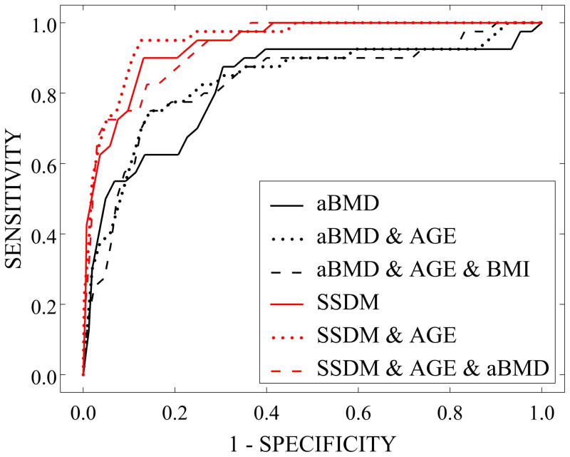
Increased risk of skeletal fractures due to bone mass loss is a major public health problem resulting in significant morbidity and mortality, particularly in the case of hip fractures. Current clinical methods based on two-dimensional measures of bone mineral density (areal BMD or aBMD) are often unable to identify individuals at risk of fracture. We investigated predictions of fracture risk based on statistical shape and density modeling (SSDM) methods using a case-cohort sample of individuals from the Osteoporotic Fractures in Men (MrOS) study. Baseline QCT data of the right femur were obtained for 513 individuals, including 45 who fractured a hip during follow-up (mean 6.9 year observation, validated by physician review). QCT data were processed for 450 individuals (including 40 fracture cases) to develop individual models describing three-dimensional bone geometry and density distribution. Comparison of mean fracture and non-case models indicated complex structural differences that appear to be responsible for resistance to hip fracture. Logistic regressions were used to model the relation of baseline hip BMD and SSDM weighting factors to the occurrence of hip fracture. Area under the receiver operating characteristic (ROC) curve (AUC) for a prediction model based on weighting factors and adjusted by age was significantly greater than AUC for a prediction model based on aBMD and age (0.94 vs. 0.83, respectively). The SSDM-based prediction model adjusted by age correctly identified 55% of the fracture cases (and 94.7% of the non-cases), whereas the clinical standard aBMD correctly identified 10% of the fracture cases (and 91.3% of the non-cases). SSDM identifies subtle changes in combinations of structural bone traits (e.g., geometric and BMD distribution traits) that appear to indicate fracture risk. Investigation of important structural differences in the proximal femur between fracture and no-fracture cases may lead to improved prediction of those at risk for future hip fracture.

INTRODUCTION

The problem of increased risk of skeletal fractures due to bone mass loss in aging or disease is a major clinical problem leading to estimated health care costs of nearly $17 billion in the US ^{[1, 2]}. Not withstanding the economic burden, non-vertebral fractures, particularly of the hip, are a significant cause of morbidity and mortality in the aging population ^[3–5]. More than 4% of hip fracture patients die during the initial hospitalization following fracture and 24% will die within the first year ^[6]. Thus, concerted efforts are needed to identify treatment strategies that can maintain the health of the skeleton with age. However, of primary importance is improving the accuracy in identification of those at risk for bone fractures.

Bone mineral density (BMD) measurements are widely used to assess bone mineral status, especially in women, and BMD can account for up to 70% of bone strength. While correlations between bone mineral density, commonly determined using dual energy x-ray absorptiometry (DXA), and fracture risk have been demonstrated, prediction models based on DXA alone often have low sensitivity in identifying individuals likely to suffer a fracture, particularly in menopausal women and in older populations ^{[7, 8]}.

The structural integrity of an individual bone in any mechanical loading environment is dependent on the spatial BMD distribution, the size and shape of the bone, as well as the material properties of the bone tissue ^{[9, 10]}. Numerous studies have investigated correlations between femur BMD and geometry and fracture risk, primarily in terms of bone strength ^[11–13]. However, it appears likely that risk predictions based on simplified measures of bone geometry (i.e., femoral neck axis length, femoral neck length, femoral neck diameter, cortical thickness, etc.) and measures of regional average BMD (i.e., femoral neck BMD, intertrochanteric BMD, total hip BMD) do not adequately describe the three dimensional combinations of bone traits that lead to the structural integrity of a bone.

Conversely, without making a priori assumptions regarding the importance of geometric descriptors or fundamental aspects of model definition, statistical shape modeling methods have been used to describe variability in the morphology of a population of anatomical structures ^[14–17]. Statistical shape models capture the high dimensional variability within a set of biological structures, such as bones, and describe the variation in structural traits (e.g., geometry and bone density distribution) in an efficient manner. In the context of biomechanics, statistical shape modeling allows investigation of the important structural differences expected to allow improved identification of those at risk.

In this study, we investigated the use of fracture risk predictions based on statistical shape and density modeling (SSDM) methods, which describe both the multivariate geometry and BMD distribution variation contained implicitly within 3D imaging data for a set of bones. The performance of SSDM-based fracture risk predictions was compared to those based on BMD alone. The ultimate goal of this research program is to generate the fundamental knowledge required to develop and implement a clinical risk assessment tool.

METHODS

Study Population

The Osteoporotic Fractures in Men (MrOS) Study is a multi-center observational study investigating the determinants of fracture in a group of older men (n=5,994, age ≥ 65) ^{[18, 19]}. Baseline areal bone mineral density (aBMD) was obtained for the total hip following standardized procedures at all study sites, including dual-energy x-xray absorptiometry (DXA) cross-calibration and daily quality control scans (QDR 4500W; Hologic) ^[20]. Hip quantitative computed tomography (QCT) image data were collected for the pelvic region extending from the femoral head to approximately 3.5 cm below the lesser trochanter. Imaging data of the hip and a hydroxyapatite (HA) density calibration phantom (Image Analysis, Columbia, KY) were collected with scanner settings of 80 kVp, 280 mA, 3 mm slice thickness, 512 × 512 in-plane array dimensions, in spiral reconstruction mode ^[21]. QCT data were available at study baseline for 3,561 individuals. After enrollment, participants were questioned by mail every four months regarding the occurrence of any recent fractures with 99% complete follow-up. Any reported hip fractures were validated by physician review of radiology reports or X-rays, if no radiology report was available.

Case-Cohort Selection

Within the follow-up period, a total of 45 hip fracture cases occurred in the group of individuals with baseline QCT data available. Based on the case-cohort sampling design, 472 individuals were randomly selected from the group with baseline QCT. However, 4 hip fracture cases occurred in the random sample, resulting in a total of 513 individuals in the case-cohort sample with an average observation period of 6.9 years. Baseline QCT and aBMD data were obtained for these men.

Processing of QCT data

All image processing was performed while blinded to fracture status. Each baseline QCT data set was segmented to extract right femur data from the QCT image data (Figure 1) (Seg3D, The Center for Integrative Biomedical Computing, University of Utah, Salt Lake City, UT). Due to image quality issues or incomplete data for the right femur, a total of 450 out of 513 image data sets were successfully processed. This resulted in a study sample containing 40 fracture cases and 410 non-cases. Closed triangulated surfaces were generated to describe the outer cortical boundary of each femur (Figure 1) (MATLAB R2012a, The Mathworks, Inc., Natick, MA).

Figure 1. Image Processing Pathway from QCT Data to Segmented Data to Femur Surface.

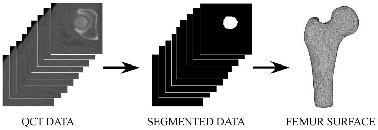
QCT data was semi-automatically segmented to generate a binary stack of image data for each individual femur. The binary stack of image data was processed to generate closed triangulated surfaces describing the outer cortical boundary of each individual femur. (Note: A subset of QCT and segmented data slices are shown here for clarity.)

Femur surfaces were aligned to the CT scan axes and transected at the inferior-most level of the lesser trochanter to generate femur surfaces proportionally sized for individual subject hip anatomy (MATLAB R2012a, The Mathworks, Inc., Natick, MA). A new set of vertices was mapped onto each femur surface and repositioned such that each femur surface was described using 4,102 vertices and all vertices were positioned at the same anatomical locations for each femur (Figure 2) ^[22]. Thus, the resulting femur surfaces were defined by the same surface mesh definition due to vertex correspondence across the set of femurs. The average femur surface was determined by averaging vertex positions for all femurs.

Figure 2. Anatomic Position of Surface Vertices Correspond for all Femur Surfaces.

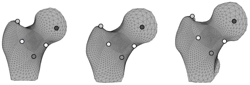
White, black, and gray dots denote corresponding surface vertices between three example femur surfaces. Note that the dots are located at the same anatomic position for each femur surface allowing the geometry of surfaces with dissimilar shapes to be directly compared.

A volumetric tetrahedral mesh (77,708 elements and 14,350 nodes) was defined for the average femur surface (Tetgen, Weierstrass Institute for Applied Analysis and Stochastics, Berlin, Germany). The average femur mesh was warped to each individual femur surface using displacement vectors calculated between corresponding surface vertices on the average femur mesh and the individual femur surfaces, resulting in a set of 450 corresponding femur mesh models (ANSYS v11.0, ANSYS, Inc., Canonsburg, PA).

Individual femur models were superimposed on CT data for the same individual and CT image intensity was determined at the spatial location of each node (MATLAB R2012a, The Mathworks, Inc., Natick, MA). The image intensity distribution for each femur was converted to a spatial distribution of equivalent solid HA concentration using a regression based on the graded HA densities within the HA phantom and image intensity data within corresponding regions of interest. Following Carpenter, et al. [23], equivalent HA concentration was converted to equivalent liquid K2HPO4 concentration [24], and then to a wet apparent bone density distribution for each individual femur [25]. This process resulted in a set of 450 femur geometry and density distribution models where each model consisted of 57,400 variables (i.e., spatial location and BMD at each mesh node).

Development of Statistical Shape and Density Model for Femur Sets

A statistical shape and density model (SSDM) ^[26] was generated to describe and investigate variability in the baseline geometry and density distribution models for the set of 450 femurs, without regard to subsequent fracture occurrence (Appendix). Using a principal component analysis, the highly correlated geometry and density variables were reduced into a relatively small set of 449 uncorrelated and independent composite geometry and BMD traits (i.e., principal components or shape modes). Each model was described as a weighted linear combination of principal components. By definition, all variability within the original set of geometry and bone density distribution models was retained and each individual femur was described by a set of 449 principal component weighting factors, rather than the original 57,400 descriptive variables.

Investigation of the Differences between Fracture Cases and Non-Case

Previous investigation has demonstrated that complex differences in proximal femur geometry and BMD distribution exist between individual bones that suffer fractures and those that do not ^[27]. Additionally, these important variations may not be captured using typical physical descriptors of bone geometry (i.e., femoral neck axis length, femoral neck diameter, neck-shaft angle, femoral head diameter) and regional measures of bone density distribution (i.e., greater trochanter or total hip BMD). To investigate the complex structural variations between fracture cases and non-cases, a mean fracture model and a mean non-case model were generated by separately averaging the weighting factors for the 40 fracture cases and the 410 non-cases (Appendix, Eqns. 4 and 6). Spatial variation in surface geometry and mid-plane BMD variation of the 3D models was quantitatively investigated by determining the trait differences at each model node. Similarly, the structural variations described by the first two shape modes were also investigated by generating models based on the mean femur modified by the mean variation in the appropriate shape mode for the fracture cases and the mean femur modified by the mean variation in the appropriate shape mode for the non-case femurs (Appendix, Eqns. 4 and 6)

Development of Risk Prediction Models

Separate risk prediction models were developed to indicate the occurrence of future fracture using predictor variables including baseline aBMD and SSDM weighting factors determined from analysis of baseline QCT data, and covariate data (Table 1). A logistic regression was used to model the relation of total hip aBMD, the current clinical gold standard, to the occurrence of hip fracture (MATLAB R2012a, The Mathworks, Inc., Natick, MA) and this relation was modified by sequentially adding age and BMI.

Table 1.

Fracture Classifier Characteristics

Fracture Classifier	Mean Number of SSDM Weighting Factors Included	Mean Percentage of Total Variability Explained by Selected Weighting Factors
Total Hip aBMD	0	0
aBMD & Age	0	0
aBMD & Age & BMI	0	0
SSDM	23.5	49.6
SSDM & Age	20	53.8
SSDM & Age & aBMD	16.6	52.9

Similarly, the relation of SSDM weighting factors to the occurrence of hip fracture was modeled with a logistic regression based on a subset of weighting factors (MATLAB R2012a, The Mathworks, Inc., Natick, MA). The number of selected weighting factors was first reduced by eliminating any weighting factors with a F-score less than the sum of the median F-score and 3 times the mean absolute deviation of the F-scores, thereby eliminating weighting factors that do not differentiate well between fracture cases and non-cases ^[28]. The lasso approach was used to further reduce the number of selected weighting factors and fit the logistic regression between the selected weighting factors and the occurrence of hip fracture ^{[29, 30]}. Baseline covariates (i.e., age, BMI, and aBMD) were sequentially added to the pool of predictor variables and logistic regressions adjusted by covariates were determined by repeating the two-level variable reduction approach.

A nested 10-fold cross-validation approach was used to develop all fracture prediction models in order to maximize reproducibility and eliminate the potential for bias and overfitting of the classifiers ^{[31, 32]}. The sample of 450 individuals was randomly partitioned into 10 equal size subsamples (i.e., “test” sets) of 45 individuals. Once a test set was selected, a fracture prediction model was defined using predictor variables for the remaining “training set” of 405 individuals, and the resulting prediction model was used to predict the occurrence of future fracture using predictor variables from the test set of individuals. This nested loop procedure was repeated 10 times (i.e., 10 folds) such that future fracture likelihood was determined using predictor variables of the individuals in each test set based on fracture prediction models established from predictor variables for the remaining 405 individuals. Stratified partitioning was employed to ensure that the training and test sets in each fold contained the same proportion of fracture cases and non-cases as in the overall sample of 450 individuals. This partitioning approach resulted in 4 fracture cases and 41 non-cases in each test set. In prediction models involving weighting factors, 10-fold cross-validation was also used in the lasso fit of the logistic regression between training set predictor variables and fracture occurrence.

Investigation of Fracture Classifier Performance

Receiver operating characteristic (ROC) curves were generated to graphically represent true positive rate (i.e., sensitivity) versus false positive rate (i.e., 1-specificity) for each prediction model in each of the 10 folds and averaged over the folds to determine the ROC for each prediction model. The area under the ROC curve (AUC) was determined from each ROC for each prediction model as a direct indicator of reliability (i.e. probability that the prediction model will rank a randomly chosen positive (i.e., correct) prediction higher than a randomly chosen negative one) and 95% confidence intervals for AUC values were computed using 1000 bootstrap replicas. Cross-validated AUC values and 95% confidence intervals for the AUC values were determined for each prediction model (cvAUC package in R, available at http://cran.r-project.org/web/packages/cvAUC/index.html) ^[33].

The predictive performance of each fracture prediction model was validated using the results of the test set predictions in the nested cross-validation approach. It follows that performance was judged on the ability of each model to predict the occurrence of fracture in a set of individuals (i.e., the test set) that were not involved in prediction model definition and that these individuals were “unknown” and external to the prediction model. Rates of overall correct prediction and correct prediction for fracture and non-case individuals were determined for the test set in each fold and averaged over the 10 folds to determine the performance of each prediction model. Significance of differences in prediction accuracy was investigated using repeated measures analyses of variance and Tukey’s test was used for between predictor comparisons, if appropriate.

The association between the accuracy of prediction models and the principal components that explained the majority of the total variance in femur geometry and bone density distribution was investigated. Three new prediction models were developed using subsets of weighting factors selected in the prediction model based on principal components and adjusted for age. Prediction models were defined using selected weighting factors that individually described greater than 10% of the total variance, weighting factors that individually described greater than 1% of the total variance, and weighting factors that individually described less than 1% of the total variance. All subset-based predictors were adjusted by age and the rates of overall correct prediction and correct prediction for fracture and non-case individuals were determined as means in a 10-fold cross-validation analysis. Significance of differences in prediction accuracy was investigated using repeated measures analyses of variance and Tukey’s test was used for between predictor comparisons, if appropriate.

RESULTS

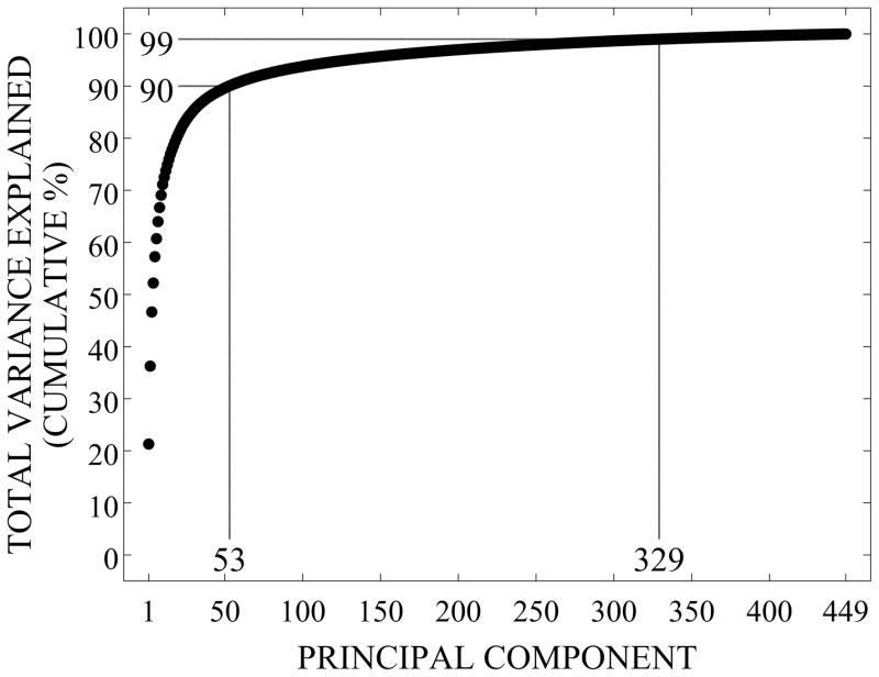
The first principal component (shape mode) of the SSDM explains 21% of the total variance in femur geometry and bone density distribution, shape modes 1–53 explain 90% of the total variance, and shape modes 1–329 explain 99% of the total variance (Figure 3). Accordingly, the remaining 120 shape modes cumulatively explain 1% of the total variance in geometry and BMD distribution.

Figure 3.

Cumulative Percentage of Femur Variability Explained by Principal Components

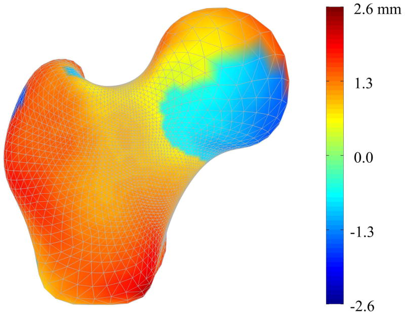
The complex pattern of structural geometry variations between the mean fracture case model and the mean non-case model is clearly demonstrated (Figure 4). Interestingly, as indicated by the red and orange regions, the mean fracture case femur model is generally larger than the mean non-case model, particularly in the distal neck, greater trochanteric, and intertrochanteric regions. The fringe pattern at the femoral head appears to demonstrate a rotation of the fracture case model femoral head with respect to that of the non-case model, indicating that the neck-axis shaft angle is greater for the fracture case than the non-case. The neck axis shaft angle and the neck diameter are greater for the mean fracture case model than for the mean non-case model. However, it remains that typical length-based measures would inadequately describe the complex variations shown.

Figure 4. Surface Geometry Variation between Mean Fracture and Non-Case Femurs.

Color contours represent the difference in shape between the mean fracture model and the mean non-case model at each surface node. Accordingly, red regions indicate that those nodes in the case model are outside the non-case model at that point, demonstrating that the mean case model is larger than the mean non-case model in these regions. Conversely, blue regions indicate that the mean case model is smaller than the mean non-case model at those points.

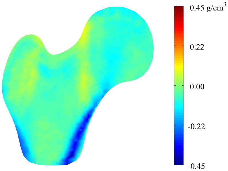
Similarly, the mid-plane density variation indicates complex differences that are difficult to completely characterize using typical regional measures of density (Figure 5). In general, the light blue and blue regions indicate that the mid-plane BMD is lower in the mean fracture case than in the mean non-case, particularly in the intertrochanteric and distal cortical regions, as well as the location of the primary compressive strut in the femoral head ^[34]. The yellow and orange regions indicate small regions of increased mid-plane BMD between the mean fracture case and the mean non-case models, although these differences are slight.

Figure 5. Mid-plane Density Variation between Mean Fracture and Non-Case Femurs.

Color contours represent pointwise density differences between the mean fracture model and the mean non-case model. Accordingly, red regions indicate that those nodes in the case model have greater density than the non-case model at that point and blue regions indicate that the mean case model has less density than the mean non-case model at those points.

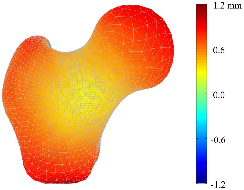
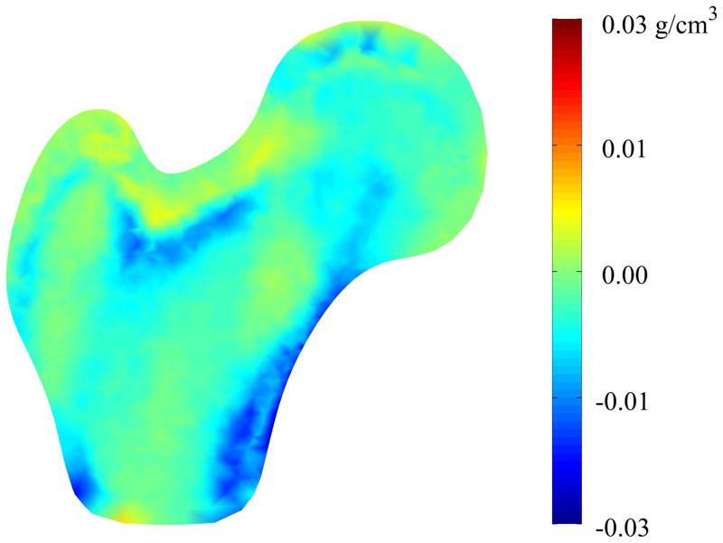
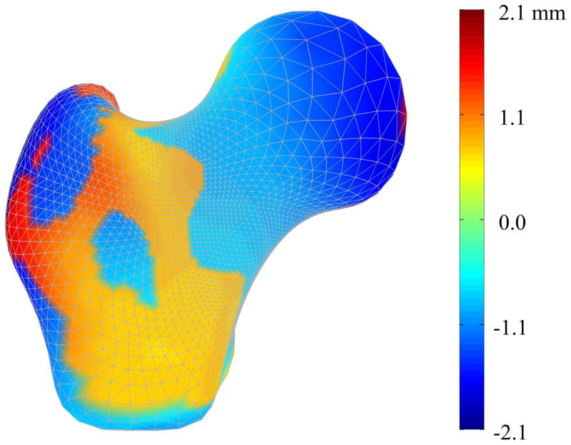
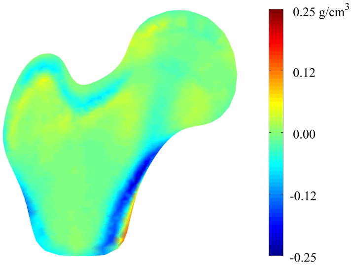
Mode 1 described increases in the femoral head diameter and the femoral neck axis length for the fracture cases when compared to non-cases, along with other more complex increases over the surface of the proximal femur (Figure 6). Mode 1 also described very minor decreases (< 0.03 g/cm³) in density along the medial cortical bone inferior to the femoral head (Figure 7). Conversely, shape mode 2 described decreases in femoral head diameter, femoral neck diameter, and femoral neck axis length for fracture cases compared to the non-cases, along with complex variation of the remaining surface (Figure 8). Shape mode 2 also described decreases in lateral and medial cortical bone density, as well as within the trabecular bone of the greater trochanter, superior femoral neck, and the primary compressive strut, for the fracture cases compared to the non-cases (Figure 9).

Figure 6. Mode 1 Surface Geometry Variation between Fracture and Non-Case Femurs.

Color contours represent the pointwise differences in shape between the mean femur modified by the mean variation in shape mode 1 for the fracture cases and the mean femur modified by the mean variation in shape mode 1 for the non-case femurs.

Figure 7. Mode 1 Mid-plane Density Variation between Fracture and Non-Case Femurs.

Color contours represent the pointwise density differences between the mean femur modified by the mean variation in shape mode 1 for the fracture cases and the mean femur modified by the mean variation in shape mode 1 for the non-case femurs.

Figure 8. Mode 2 Surface Geometry Variation between Fracture and Non-Case Femurs.

Color contours represent the pointwise differences in shape between the mean femur modified by the mean variation in shape mode 2 for the fracture cases and the mean femur modified by the mean variation in shape mode 2 for the non-case femurs.

Figure 9. Mode 2 Mid-plane Density Variation between Fracture and Non-Case Femurs.

Color contours represent the pointwise density differences between the mean femur modified by the mean variation in shape mode 2 for the fracture cases and the mean femur modified by the mean variation in shape mode 2 for the non-case femurs.

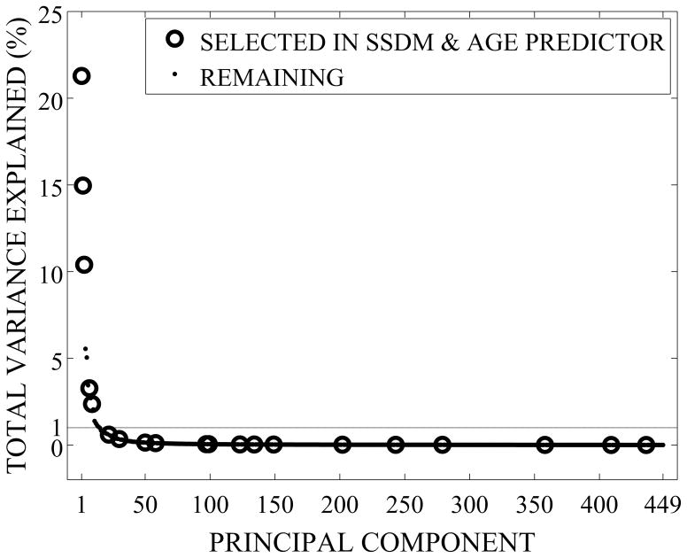
The two-level predictor selection approach identified an average number of discriminative weighting factors ranging from 16.6 to 23.5 weighting factors out of 449 (Table 1). Adjusting the SSDM-based risk prediction model by age reduced the average number of selected weighting factors from 23.5 to 20 and further adjusting the model by aBMD reduced the average number to 16.6, suggesting that discriminative information contained within some weighting factors could be replaced by covariate adjustment. BMI was not selected as a discriminative predictor in logistic regressions containing SSDM weighting factors. Interestingly, prediction models defined using the nested cross-validation approach were based on selected weighting factors describing between 49.6 and 53.8% of the total model variability. Furthermore, prediction models primarily included principal components describing a small percentage of the total variation in geometry and BMD distribution for the set of 450 femurs. For instance, the risk prediction model containing SSDM weighting factors and age contained 3 weighting factors that cumulatively described 46.7% of the total variability and 17 weighting factors that cumulatively described 7.1% of the total model variability (Figure 10).

Figure 10.

Percentage of Femur Variability Explained by Individual Principal Components

ROC curves demonstrated that both the sensitivity and specificity of future fracture prediction increased substantially with the inclusion of SSDM weighting factors over that of aBMD alone or of aBMD adjusted by age and BMI (Figure 11). Accordingly, AUC values indicating prediction reliability were significantly greater in prediction models including weighting factors than those without (Table 2). Adjustment of the SSDM-based fracture prediction model by covariate characteristics resulted in slight variation in the AUC values from that of SSDM alone.

Figure 11.

Receiver Operating Characteristic (ROC) Curves for Cross-Validated Fracture Prediction Models

Table 2.

Reliability of Fracture Prediction Models

Fracture Prediction Model	AUC (95% C.I.)
Total Hip aBMD	0.82 (0.75 – 0.89)
aBMD & Age	0.83 (0.77 – 0.90)
aBMD & Age & BMI	0.83 (0.77 – 0.89)
SSDM	0.94 (0.91 – 0.97)
SSDM & Age	0.94 (0.91 – 0.97)
SSDM & Age & aBMD	0.93 (0.90 – 0.96)

Cross-validation analyses were performed using aBMD-based risk prediction (as the clinical gold standard) with adjustment by age and BMI and the fracture predictors determined using SSDM weighting factors (Table 3). The overall accuracy for the SSDM-based predictor adjusted for age was significantly greater than the overall accuracy for all aBMD-based measures (p-value = 0.000). The accuracies of all SSDM-based fracture classifications were significantly greater than the accuracies of all aBMD-based measures (p-value = 0.000). There were no significant differences in the accuracy of identifying non-case individuals (p-value = 0.925)

Table 3.

Validation of Fracture Prediction Model Accuracy

Fracture Classifier	Mean Correct Classifications (out of 45 men)	Mean Correct Fracture Classifications (out of 4 men)	Mean Correct Non-case Classifications (out of 41 men)
Total Hip aBMD	41.1 (91.3%)	0.4 (10.0%)	40.7 (99.3%)
aBMD & Age	41.1 (91.3%)	0.6 (15.0%)	40.5 (98.8%)
aBMD & Age & BMI	41.0 (91.1%)	0.6 (15.0%)	40.4 (98.5%)
SSDM	42.1 (93.6%)	1.6 (40.0%)	40.5 (98.8%)
SSDM & Age	42.6 (94.7%)	2.2 (55.0%)	40.4 (98.5%)
SSDM & Age & aBMD	42.1 (93.6%)	1.7 (42.5%)	40.4 (98.5%)

A subset of three weighting factors selected in the SSDM-based predictor adjusted for age [SSDM & Age] individually explained greater than 10% of the total variance in the set of femurs and cumulatively described 46.7% of the total variance [SSDM (WFs > 10%) & Age] (Table 4). Five weighting factors individually described greater than 1% of the total variance and cumulatively described 52.3% of the total variance [SSDM (WFs > 1%) & Age]. The remaining 15 weighing factors individually described less than 1% of the total variance and cumulatively described 1.5% of the total variance [SSDM (WFs < 1%) & Age].

Table 4.

Characteristics of Fracture Classifiers based on Subsets of Weighting Factors

Fracture Classifier	Number of SSDM Weighting Factors Included	Total Variability Explained by Selected Weighting Factors
SSDM & Age	20	53.8
SSDM (WFs > 10%) & Age	3	46.7
SSDM (WFs > 1%) & Age	5	52.3
SSDM (WFs < 1%) & Age	15	1.5

Note: Parenthetical descriptions of weighting factor subsets refer to the variability that is explained individually by each principal component weighting factor. For instance, there are 3 weighting factors that each describe greater than 10% of the total variability in the set of femurs.

Cross-validation analyses were performed to compare the accuracy of the SSDM & Age fracture risk predictor to predictors defined using subsets of these weighting factors and adjusted by age (Table 5). Overall accuracy for the SSDM & Age predictor was significantly greater than overall accuracy for SSDM (WFs> 10%) & Age, but was not significantly different than overall accuracy for SSDM (WFs < 1%) & Age and SSDM (WFs < 1%) & Age (p-value = 0.012). Accuracy for fracture classifications using SSDM & Age was not significantly different from the accuracy for SSDM (WFs < 1%) & Age; however, it was significantly greater than the accuracy for fracture classifications using SSDM (WFs > 10%) & Age and SSDM (WFs > 1%) & Age (p-value = 0.001). There were no significant differences in accuracy for prediction of the non-case individuals (p-value = 0.627).

Table 5.

Accuracy of Fracture Prediction Model based on Subsets of Weighting Factors

Fracture Classifier	Mean Correct Classifications (out of 45 men)	Mean Correct Fracture Classifications (out of 4 men)	Mean Correct Non-case Classifications (out of 41 men)
SSDM & Age	42.6 (94.7%)	2.2 (55.0%)	40.4 (98.5%)
SSDM (WFs > 10%) & Age	40.8 (90.7%)	0.4 (10.0%)	40.4 (98.5%)
SSDM (WFs > 1%) & Age	41.2 (91.6%)	1.1 (27.5%)	40.1 (97.8%)
SSDM (WFs < 1%) & Age	42.1 (93.6%)	1.5 (37.5%)	40.6 (99.0%)

Notes: Parenthetical descriptions of weighting factor subsets refer to the variability that is explained individually by each principal component weighting factor.

DISCUSSION

Quantitative differences in baseline proximal femur geometry and BMD distribution exist between older men that subsequently suffer a hip fracture and those do not, and these variations are complex. Using imaging processing methods, the baseline variability in the proximal femurs of fracture and non-fracture cases was described by high fidelity models composed of a set of highly correlated variables describing proximal femur shape and bone density distribution. In turn, the highly correlated variables were transformed using a variable reduction method (i.e., principal component analysis) into a relatively small set of new composite trait variables (i.e., principal components or shape modes) that described independent and uncorrelated combinations of geometry and BMD distribution.

SSDM provides a means of explicitly describing baseline variation between individuals that subsequently suffer a hip fracture and those that do not, suggesting that the statistical investigation of composite bone traits that differ between these individuals may lead to improved methods of fracture risk diagnosis. Statistical shape and density modeling methods describe inherent combinations of traits related to three-dimensional bone shape and the spatial distribution of bone mineral density that are found within bones. The unsupervised means of disseminating highly correlated shape and density variables into composite traits identifies hidden structural combinations within the shape and density data that are directly related to fracture risk. We note that composite bone traits do not have explicit physical meaning, as they are combinations of observable bone traits; however, differences in baseline composite traits between individuals that suffer a hip fracture and those that do not can be qualitatively examined, as shown in the present study. Moreover, composite bone traits represent an integrated view and an important starting point for investigation of the importance of not only multiple observable bone traits, but also of the significance of the essential interactions between bone traits with regards to structural integrity and fracture resistance of the bone. As demonstrated in the current study, fracture risk predictions for a small set of individuals (i.e., the test set) are based on the similarity of SSDM weighting factors for the proximal femur of test individual(s) to those of individuals in the training set that have suffered a fracture. It follows that identical methods could be applied to individuals in the clinic to determine the risk of subsequent fracture.

Importantly, the results of this study demonstrate that subtle differences between bones that are described using SSDM weighting factors may predict the likelihood to suffer a subsequent fracture. It seems likely that variation in both geometry and BMD density distribution described by SSDM methods directly relates to the structural integrity of an individual bone. Accordingly, SSDM methods may lead to means of identifying individuals at risk for suffering a fracture and improving the understanding of fracture pathophysiology. Furthermore, SSDM methods may help in identifying the complex composite traits that appear to be deficient in individuals at risk and focusing on treatments that address structural deficiencies.

Although the analyses described here represent a comprehensive analysis of the variation of structural bone traits in a large (n=450) set of individuals, all of those individuals are men and, are predominantly Caucasian. As such, further work is necessary to expand these investigations to include females and other ethnicities in order to understand important sex- or ethnicity-based structural differences that may also lead to variation in fracture risk and the mechanisms likely to cause fracture in these individuals. The case-cohort sample in the present study included only 40 fracture cases and further work is necessary to understand the important structural trait variations that may surface in a larger sample of fracture cases. Further investigation is also needed to understand how variation within the sample of individuals that suffered fractures leads to varying fracture mechanisms and/or locations in the occurrence of hip fractures. Additionally, the radiation exposure associated with 3D QCT scans using current clinical scanners is approximately 1 to 3 mSv, which is two orders of magnitude greater than that of a DXA scan (0.009 – 0.013 mSv) and also greater than that associated with standard radiography (0.3 – 0.7 mSv) [35]. Although the risks of radiation doses associated with assessing bone mineral density or collecting three-dimensional QCT data are uncertain, the radiation doses associated with determining bone condition are low and it is likely that potential risks to an individual are low [35]. However, further work is needed to reduce the radiation dose with clinical QCT, and scan parameters and automatic exposure control tools may provide viable means of reducing the radiation exposure. We also acknowledge that replication of analyses of fracture risk classifiers based on statistical shape and density modeling using independent populations is an important step in the development of these risk classification methods, despite the predictive accuracy demonstrated for “unknown” test individuals in the present study.

A similar statistical shape model (SSM) approach was employed to predict incident hip fracture in a nested case-control study of white women 65 years and older^[36]. A two-dimensional (2D) statistical shape model was generated to describe the variation in proximal femur shape determined from baseline hip radiographs of 399 individuals (168 fracture cases, 231 controls). Shape modes based on the outer 2D boundary of the proximal femur resulted in more accurate prediction of the occurrence of future hip fractures than BMD or FRAX scores. The AUC for the fracture classifier based on shape modes and adjusted by femoral neck BMD was 0.835, compared to 0.813 for shape modes alone and 0.675 for femoral neck BMD alone and 0.645 for intertochanteric BMD alone. Another study utilized baseline DXA scans of the hip from elderly women aged 75 years or older, including 182 fracture cases and 364 controls [37]. Active shape models (a.k.a. statistical shape models) were developed from corresponding points located on the proximal femur and parts of the pelvis and active appearance models were developed to describe the 2D distribution of bone mineral density within the femoral head and neck. Fracture risk predictors based on shape and appearance modes resulted in AUC values ranging from 0.57 to 0.65, and no predictor resulted in an AUC value that was significantly different than that of total hip BMD alone (AUC = 0.62). A third study utilized regional fast Fourier transform-based texture analyses and fractal analyses of hip radiographs previously obtained for a set of postmenopausal women (26 hip fracture cases and 24 controls) [38]. Statistical shape modeling was used to model the shape of power spectrum texture profiles, rather than femoral geometry. Regional texture modes and fractal dimensions were used to develop fracture risk predictors that resulted in AUC measures ranging from 0.59 to 0.93, where the maximum AUC value was achieved for a predictor based on lower femoral neck texture. Although this study utilized a small sample set, prediction accuracy rates were not reported, and the lack of nested cross-validation to limit the potential for predictor bias suggest that texture analysis of the lower femoral neck may hold promise as a fracture risk predictor. However, it is unclear whether lower femoral neck texture will show similar performance for the full range of fracture types and locations. In comparison to fracture risk predictors based on statistical modeling of 2D imaging data, cross-validated AUC values ranged from 0.93 to 0.94 for SSDM-based classifiers in the present study, suggesting that description of the 3D geometry and spatial distribution of BMD play an important role in the prediction of future hip fractures.

A study involving 3D QCT data implemented voxel-based morphometry to compare the femoral BMD distribution between groups of individuals that suffered a subsequent fracture and those that did not ^[39]. Voxel-based morphometry relies on a comparison of BMD at each voxel over BMD distributions that are warped to a common “atlas.” In effect, variations in the spatial distribution of BMD are considered, but variations in geometry between individuals and groups are not, although Carballido-Gamio, et al., considered overall changes in geometry scale. Decreased BMD was noted along the endosteal cortical region of both the superior and inferior cortices of the femoral neck of women with subsequent fracture. This finding parallels the results of the present study considering men with and without subsequent fracture, suggesting that cortical bone loss patterns may be similar in both males and females that suffer fracture. Additionally, females that suffer subsequent fracture have greater femoral neck diameter than those that do not, which again parallels findings in the current study comparing males with and without subsequent fracture. Increases in femoral neck size in individuals with subsequent fracture seem likely to be a response intending to offset patterns of decrease in neck BMD ^[39].

As fracture is a structural failure of the bone, numerous studies have employed finite element methods to determine peak expected strain, strength, or load-to-strength ratio in order to develop fracture risk predictors. One such study employed two-dimensional finite element models developed from DXA imaging data of the femur previously obtained from 93 white women, 42 of whom suffered a subsequent hip fracture [40]. Elastic material properties were assigned based on density distribution, fall-type loading conditions were employed and principal strains were calculated for each femur. A fracture risk predictor based on femoral neck BMD had an overall accuracy of 64.5%, a predictor based on femoral neck BMD and height had an overall accuracy of 76.3%, and adding neck shaft angle and maximum principal tensile strain increased the overall accuracy to 81.7%, although 82.9% of the fracture cases were correctly identified. A similar study defined finite element models of the proximal femur using baseline DXA data obtained for 728 women aged 75 years or older, including 182 that suffered a subsequent hip fracture [41]. Fracture risk predictors based on femoral neck BMD, estimated femoral strength, and load-to-strength ratio resulted in AUC values ranging 0.66 for BMD alone to 0.68 for load-to-strength ratio. Adjusting estimated strength and load-to-strength ratio by femoral neck BMD resulting in AUC values of 0.68 and 0.69, respectively. AUC values for predictors were not significantly different than that of BMD alone (95% significance level). A third study implemented 3D finite element models using baseline QCT data for a subset of 250 individuals in the present study [20]. Elastic-plastic material properties were assigned based on density distribution and strength of the proximal femur under fall loading conditions and load-to-strength ratio were calculated and used to define fracture risk predictors. Predictors based on femoral strength, load-to-strength ratio, and total hip aBMD resulted in AUC values of 0.83, 0.79, and 0.85, respectively. After accounting for age, BMI, and clinical center in the predictors, AUC values increased slightly to 0.87 for femoral strength, 0.88 for load-to-strength ratio, and 0.88 for aBMD alone, although differences in the results were not significant. Decreased accuracy when compared to the present study and lack of significant differences between predictors based on finite element model results and those of BMD alone suggest that modeling choices and assumptions do play an important role in determining the likelihood of future fracture occurrence. It remains unclear how sensitive relative changes in accuracy of the finite element model predictions are to modeling choices, as well as how well finite element-based strength predictions can accurately predict the likelihood of subsequent fracture in a living individual. As noted previously, the statistical shape and density modeling approach does not make a priori assumptions in developing a predictive classifier. Rather, the SSDM approach describes the available data on proximal femur shape and BMD distribution in an unsupervised manner and is trained to generate a classifier based on consideration of the relation of shape mode weighting factors to fracture occurrence.

In conclusion, statistical shape and density modeling provides a means of explicitly and efficiently describing the complex spatial variation in geometry and BMD distribution within a sample of proximal femurs. Statistical shape and density modeling allows for determination of complex combinations of structural bone traits that appear to indicate fracture risk and may help to differentiate at risk individuals within a sample population. Finally, description of bone sample variation using SSDM allows investigation of important structural differences that may allow improved prediction of those at risk for future hip fracture.

APPENDIX

Joint point distribution models were constructed from all individual mesh models. Model geometry and the spatial density distribution for each individual were described by a shape and density parameter vector as

$${\mathit{p}}_{\mathit{i}}={(v_{1x},v_{1y},v_{1z},v_{1d},\dots ,v_{jx},v_{jy},v_{jz},v_{jd})}^{\mathbf{T}}$$ (1)

where v_j(xyz) are the three-dimensional coordinates of the nodes in the volumetric mesh, v_jd is the bone density at that node, j =1,…, 14,350 nodes in the volumetric mesh, and i = 1 …n = 450 denote each femur in the set. In order to account for disparate units (i.e. location and density) in the vector and large differences in the variance of the variables, all individual shape and density parameter vectors, p_i, were normalized by dividing each variable by the standard deviation of that variable calculated for the set of 450 individuals.

The mean shape and bone density distribution of all femurs in the set was defined as

$$\overline{\mathit{p}}=\frac{1}{n}\sum _{i=1}^n{\mathit{p}}_i$$ (2)

and the correlation between individual models in the set was given by the empirical covariance matrix

$$\mathit{S}=\frac{1}{n}\sum _{i=1}^n\left({\mathit{p}}_i-\overline{\mathit{p}}\right){\left({\mathit{p}}_i-\overline{\mathit{p}}\right)}^T$$ (3)

A principal components analysis (PCA) of the covariance matrix, S, resulted in a set of k = n−1 eigenvalues (λ_k) and eigenvectors (q_k), which are the principal directions spanning a shape and bone density space centered at the mean, $\overline{\mathit{p}}$. The proportion of the total variance described along each eigenvector is equal to its corresponding eigenvalue divided by the sum of all eigenvalues; eigenvectors corresponding to the largest eigenvalues describe the majority of the variance (Figure 3). Thus, geometry and density distribution models for each femur in the set were described in terms of the average model and a weighted linear combination of uncorrelated principal shape and bone density modes as

$${\mathit{p}}_i=\overline{\mathit{p}}+\sum _k{b}_{ik}{\mathit{q}}_k$$ (4)

where for each individual femur

$${\mathit{b}}_i={\mathit{Q}}^T\left({\mathit{p}}_i-\overline{\mathit{p}}\right)$$ (5)

are the score vectors that are functions of the eigenvalues and Q^T contains the k eigenvectors. Weighting factors for each individual model were determined by dividing the k scores by the square root of the corresponding eigenvalue

$$c_{ik}=\frac{b_{ik}}{\sqrt{{\lambda }_k}}$$ (6)

where $\sqrt{{\lambda }_k}$ is the standard deviation of the shape and density distribution from the mean along the corresponding eigenvector.

References

- 1.Burge R, Dawson-Hughes B, Solomon DH, Wong JB, King A, Tosteson A. Incidence and economic burden of osteoporosis-related fractures in the United States, 2005–2025. J Bone Miner Res. 2007;22(3):465–475. doi: 10.1359/jbmr.061113. [DOI] [PubMed] [Google Scholar]
- 2.Kanis JA, Johnell O, Oden A, et al. Long-term risk of osteoporotic fracture in Malmo. Osteoporos Int. 2000;11(8):669–674. doi: 10.1007/s001980070064. [DOI] [PubMed] [Google Scholar]
- 3.Zhou Z, Radaelli A, Johnell O, Willke RJ, Massimini G. A retrospective analysis of health care costs for bone fractures in women with early-stage breast carcinoma. Cancer. 2004;100(3):507–517. doi: 10.1002/cncr.11917. [DOI] [PubMed] [Google Scholar]
- 4.Kayan K, Kanis J, McCloskey E. Osteoporosis management by geriatricians in the UK. Age Ageing. 2003;32(5):553. doi: 10.1093/ageing/afg085. [DOI] [PubMed] [Google Scholar]
- 5.Khosla S, Melton LJ, 3rd, Dekutoski MB, Achenbach SJ, Oberg AL, Riggs BL. Incidence of childhood distal forearm fractures over 30 years: a population-based study. JAMA. 2003;290(11):1479–1485. doi: 10.1001/jama.290.11.1479. [DOI] [PubMed] [Google Scholar]
- 6.Wolinsky FD, Fitzgerald JF, Stump TE. The effect of hip fracture on mortality, hospitalization, and functional status: a prospective study. Am J Public Health. 1997;87(3):398–403. doi: 10.2105/ajph.87.3.398. [DOI] [PMC free article] [PubMed] [Google Scholar]
- 7.Kanis JA. Diagnosis of osteoporosis and assessment of fracture risk. Lancet. 2002;359(9321):1929–1936. doi: 10.1016/S0140-6736(02)08761-5. [DOI] [PubMed] [Google Scholar]
- 8.Kanis JA, Black D, Cooper C, et al. A new approach to the development of assessment guidelines for osteoporosis. Osteoporos Int. 2002;13(7):527–536. doi: 10.1007/s001980200069. [DOI] [PubMed] [Google Scholar]
- 9.Jepsen KJ, Hu B, Tommasini SM, et al. Genetic randomization reveals functional relationships among morphologic and tissue-quality traits that contribute to bone strength and fragility. Mammalian Genome. 2007;18(6–7):492–507. doi: 10.1007/s00335-007-9017-5. [DOI] [PMC free article] [PubMed] [Google Scholar]
- 10.Tommasini SM, Nasser P, Hu B, Jepsen KJ. Biological co-adaptation of morphological and composition traits contributes to mechanical functionality and skeletal fragility. J Bone Miner Res. 2008;23(2):236–246. doi: 10.1359/JBMR.071014. [DOI] [PMC free article] [PubMed] [Google Scholar]
- 11.Cheng XG, Lowet G, Boonen S, et al. Assessment of the strength of proximal femur in vitro: relationship to femoral bone mineral density and femoral geometry. Bone. 1997;20(3):213–218. doi: 10.1016/s8756-3282(96)00383-3. [DOI] [PubMed] [Google Scholar]
- 12.Pulkkinen P, Eckstein F, Lochmuller EM, Kuhn V, Jamsa T. Association of geometric factors and failure load level with the distribution of cervical vs. trochanteric hip fractures. J Bone Miner Res. 2006;21(6):895–901. doi: 10.1359/jbmr.060305. [DOI] [PubMed] [Google Scholar]
- 13.Pulkkinen P, Jamsa T, Lochmuller EM, Kuhn V, Nieminen MT, Eckstein F. Experimental hip fracture load can be predicted from plain radiography by combined analysis of trabecular bone structure and bone geometry. Osteoporosis Int. 2008;19(4):547–558. doi: 10.1007/s00198-007-0479-9. [DOI] [PubMed] [Google Scholar]
- 14.Cootes TF, Hill A, Taylor CJ, Haslem J. Use of active shape models for locating structure in medical images. Image and Vision Computing. 1994;12:355–365. [Google Scholar]
- 15.Kaus MR, Pekar V, Lorenz C, Truyen R, Lobregt S, Weese J. Automated 3-D PDM construction from segmented images using deformable models. IEEE Trans Med Imaging. 2003;22(8):1005–1013. doi: 10.1109/TMI.2003.815864. [DOI] [PubMed] [Google Scholar]
- 16.Lorenz C, Krahnstöver N. Generation of point-based 3D statistical shape models for anatomical objects. Computer Vision and Image Understanding. 2000;77(2):175–191. [Google Scholar]
- 17.Rueckert D, Frangi AF, Schnabel JA. Automatic construction of 3-D statistical deformation models of the brain using nonrigid registration. IEEE Trans Med Imaging. 2003;22(8):1014–1025. doi: 10.1109/TMI.2003.815865. [DOI] [PubMed] [Google Scholar]
- 18.Blank JB, Cawthon PM, Carrion-Petersen ML, et al. Overview of recruitment for the osteoporotic fractures in men study (MrOS) Contemp Clin Trials. 2005;26(5):557–568. doi: 10.1016/j.cct.2005.05.005. [DOI] [PubMed] [Google Scholar]
- 19.Orwoll E, Blank JB, Barrett-Connor E, et al. Design and baseline characteristics of the osteoporotic fractures in men (MrOS) study--a large observational study of the determinants of fracture in older men. Contemp Clin Trials. 2005;26(5):569–585. doi: 10.1016/j.cct.2005.05.006. [DOI] [PubMed] [Google Scholar]
- 20.Orwoll ES, Marshall LM, Nielson CM, et al. Finite element analysis of the proximal femur and hip fracture risk in older men. J Bone Miner Res. 2009;24(3):475–483. doi: 10.1359/JBMR.081201. [DOI] [PMC free article] [PubMed] [Google Scholar]
- 21.Marshall LM, Lang TF, Lambert LC, et al. Dimensions and volumetric BMD of the proximal femur and their relation to age among older U.S. men. J Bone Miner Res. 2006;21(8):1197–1206. doi: 10.1359/jbmr.060506. [DOI] [PubMed] [Google Scholar]
- 22.Heimann T, Oguz I, Wolf I, Styner M, Meinzer H-P. Implementing the automatic generation of 3D statistical shape models with ITK. The Insight Journal; MICCAI Open Science Workshop; 2006. [Google Scholar]
- 23.Carpenter RD, Beaupré GS, Lang TF, Orwoll ES, Carter DR. New QCT analysis approach shows the importance of fall orientation on femoral neck strength. J Bone Miner Res. 2005;20(9):1533–1542. doi: 10.1359/JBMR.050510. [DOI] [PubMed] [Google Scholar]
- 24.Faulkner KG, Glüer CC, Grampp S, Genant HK. Cross-calibration of liquid and solid QCT calibration standards: corrections to the UCSF normative data. Osteoporos Int. 1993;3(1):36–42. doi: 10.1007/BF01623175. [DOI] [PubMed] [Google Scholar]
- 25.Lotz JC, Gerhart TN, Hayes WC. Mechanical properties of trabecular bone from the proximal femur: a quantitative CT study. J Comput Assist Tomogr. 1990;14(1):107–114. doi: 10.1097/00004728-199001000-00020. [DOI] [PubMed] [Google Scholar]
- 26.Nicolella DP, Bredbenner TL. Development of a parametric finite element model of the proximal femur using statistical shape and density modeling. Comput Methods Biomech Biomed Engin. 2012;15(2):101–110. doi: 10.1080/10255842.2010.515984. [DOI] [PMC free article] [PubMed] [Google Scholar]
- 27.Bredbenner TL, Mason RL, Havill LM, Orwoll S, Nicolella DP. Investigating fracture risk classifiers based on statistical shape and density modeling and the MrOS data set. Orthopaedic Research Society: Proceedings of the Annual Meeting of the Orthopaedic Research Society; San Francisco, CA. 2012. [Google Scholar]
- 28.Chen Y-W, Lin C-J. Combining SVMs with various feature selection strategies. In: Guyon I, et al., editors. Feature Extraction: Foundations and Applications. Springer-Verlag; Berlin: 2006. pp. 315–324. [Google Scholar]
- 29.Tibshirani R. Regression shrinkage and selection via the lasso. Journal of the Royal Statistical Society, Series B. 1996;58(1):267–288. [Google Scholar]
- 30.Hastie T, Tibshirani R, Friedman J. The Elements of Statistical Learning. Springer; New York: 2008. [Google Scholar]
- 31.Ambroise C, McLachlan GJ. Selection bias in gene extraction on the basis of microarray gene-expression data. Proc Natl Acad Sci U S A. 2002;99(10):6562–6566. doi: 10.1073/pnas.102102699. [DOI] [PMC free article] [PubMed] [Google Scholar]
- 32.Ruschhaupt M, Huber W, Poustka A, Mansmann U. A compendium to ensure computational reproducibility in high-dimensional classification tasks. Stat Appl Genet Mol Biol. 2004;3:Article 37. doi: 10.2202/1544-6115.1078. [DOI] [PubMed] [Google Scholar]
- 33.LeDell E, Petersen ML, van der Laan MJ. UC Berkeley Division of Biostatistics Working Paper Series. 2012. Computationally Efficient Confidence Intervals for Cross-validated Area Under the ROC Curve Estimates. [DOI] [PMC free article] [PubMed] [Google Scholar]
- 34.Stiehl JB, Jacobson D, Carrera G. Morphological analysis of the proximal femur using quantitative computed tomography. Int Orthopaedics. 2007;31:287–292. doi: 10.1007/s00264-006-0182-z. [DOI] [PMC free article] [PubMed] [Google Scholar]
- 35.Damilakis J, Adams JE, Guglielmi G, Link TM. Radiation exposure in X-ray-based imaging techniques used in osteoporosis. European Radiology. 2010;20:2707–2714. doi: 10.1007/s00330-010-1845-0. [DOI] [PMC free article] [PubMed] [Google Scholar]
- 36.Baker-LePain JC, Luker KR, Lynch JA, Parimi N, Nevitt MC, Lane NE. Active shape modeling of the hip in the prediction of incident hip fracture. J Bone Miner Res. 2011;26(3):468–474. doi: 10.1002/jbmr.254. [DOI] [PMC free article] [PubMed] [Google Scholar]
- 37.Goodyear SR, Barr RJ, McCloskey E, et al. Can we improve the prediction of hip fracture by assessing bone structure using shape and appearance modelling? Bone. 2013;53:188–193. doi: 10.1016/j.bone.2012.11.042. [DOI] [PubMed] [Google Scholar]
- 38.Gregory JS, Stewart A, Undrill PE, Reid DM, Aspden RM. Identification of hip fracture patients from radiographs using Fourier analysis of the trabecular structure: A cross-sectional study. BMC Medical Imaging. 2004;4(4):1–11. doi: 10.1186/1471-2342-4-4. [DOI] [PMC free article] [PubMed] [Google Scholar]
- 39.Carballido-Gamio J, Harnish R, Saeed I, et al. Proximal femoral density distribution and structure in relation to age and hip fracture risk in women. J Bone Miner Res. 2013;28(3):537–546. doi: 10.1002/jbmr.1802. [DOI] [PMC free article] [PubMed] [Google Scholar]
- 40.Testi D, Viceconti M, Cappello A, Gnudi S. Prediction of hip fracture can be significantly improved by a single biomedical indicator. Annals of Biomedical Engineering. 2002;30:801–807. doi: 10.1114/1.1495866. [DOI] [PubMed] [Google Scholar]
- 41.Naylor KE, McCloskey EV, Eastell R, Yang L. Use of DXA-based finite element analysis of the proximal femur in a longitudinal study of hip fracture. Journal of Bone and Mineral Research. 2013;28(5):1014–1021. doi: 10.1002/jbmr.1856. [DOI] [PubMed] [Google Scholar]