Assessing the Availability of Users to Engage in Just-in-Time Intervention in the Natural Environment

Abstract

Wearable wireless sensors for health monitoring are enabling the design and delivery of just-in-time interventions (JITI). Critical to the success of JITI is to time its delivery so that the user is available to be engaged. We take a first step in modeling users’ availability by analyzing 2,064 hours of physiological sensor data and 2,717 self-reports collected from 30 participants in a week-long field study. We use delay in responding to a prompt to objectively measure availability. We compute 99 features and identify 30 as most discriminating to train a machine learning model for predicting availability. We find that location, affect, activity type, stress, time, and day of the week, play significant roles in predicting availability. We find that users are least available at work and during driving, and most available when walking outside. Our model finally achieves an accuracy of 74.7% in 10-fold cross-validation and 77.9% with leave-one-subject-out.

INTRODUCTION

Mobile technology has a potential to provide unprecedented visibility into the health status of users in their natural environment [29]. Sensors embedded in smart phones (e.g., GPS, microphone), and wireless sensors worn on the body (e.g., electrocardiography (ECG), accelerometers) can continuously monitor an individual’s health, behavior, and the surrounding environment. Machine learning algorithms have been developed to obtain measures of behavior and exposure to the environment such as activity from accelerometers, geo-exposure from GPS, stress from physiology, and social context from microphone. These automated measures of behavioral and environmental contexts enable the design of just-intime interventions (JITI) to support maintenance of healthy behaviors. However, the success of JITI depends on timing the delivery of intervention so that users are available physically, cognitively, and socially to attend to the intervention.

We use smoking cessation to illustrate the potential of JITI and the importance of timing the delivery of JITI. Smoking is responsible for most deaths in the US, accounting for one in five deaths [34]. Although majority of daily smokers want to quit, less than 10% succeed according to Center for Disease Control. The highest lapse rate among newly abstinent smokers is in the first week when over 50% of them lapse [1]. Smoking lapse is impulsive and the first lapse usually leads to full relapse [47]. Hence, it is critical to help abstinent smokers break their urge when and where it occurs (within first few days of quitting). Although wearable sensors now provide us an ability to detect the potential precipitants (e.g., stress [40] or smoking cues detected via smart eyeglasses) and trigger a JITI to break the urge, but it will succeed only if the user is available to be engaged when the JITI is delivered. Otherwise, we may lose the precious opportunity to prevent the potent first lapse. Hence, timing a JITI is critical.

Considerable research have been conducted in a closely related topic of interruptibility [13, 23]. These works largely aim to detect interruptibility of a user at workplace by analyzing the user’s computer activity (e.g., key stokes), workplace status via audio and/or video capture of the workplace, phone status, and physical activity status via wearable sensors. Research on interruptibility provides insights about tasks or social contexts where a person is more interruptible, however, lessons from these studies cannot adequately guide the design of JITIs. This is because, unlike the case of interruption that may disrupt concentration of a task, JITI is aimed at improving the user’s health and require appropriate engagement of the user. Further, these works asked users to rate their availability in-the-moment. Such reports are subjective, can become an additional source of disruption, and do not assess user’s capability to engage in a JITI.

In this paper, we develop a model to predict availability in the natural environment. Our model is derived from data collected from a week-long mobile health study with 30 participants. During the study, participants wore a wireless physiological sensor suite that collected ECG, respiration, and accelerometry, and carried a smart phone that included GPS and accelerometers. Participants were prompted by a smartphone to complete Ecological Momentary Assessment (EMA) self-reports consisting of 42 items, multiple times daily. Answering these 42-items required a level of engagement expected in JITI. Each EMA was associated with micro-incentive to encourage compliance [36].

To address the biases in human estimates of availability [4], we use delay in responding to EMA as an objective metric to measure the availability of a participant. To predict availability, we use GPS traces to identify participants’ location and driving state, infer their physical activity states from on-body accelerometers, and stress from ECG and RIP sensor data. In addition, we use time of day, day of the week, and self-reported affect, activity type, and conversation status. We compute a total of 99 features.

We identify 30 most discriminating features and train a machine learning model to predict the availability of a user. We find that several features derived from sensors such as location, activity type, time, and day of the week, play significant roles in predicting availability. In particular, features derived from stress (inferred from physiological sensors) play a significant role in predicting availability. We find that the machine learning model can predict availability with 74.7% accuracy (against a base accuracy of 50%). This compares favorably against existing works on predicting interruptibility, where the prediction accuracy was reported to be 79.5% against a base accuracy of 70.1% in the office environment [14], and an accuracy of 77.85% against a base accuracy of 77.08% in the natural environment [42]. We find that users are usually available when walking outside of their home or work, or even if just outside of their home or work location. But, they are usually not available when driving or at work. We also find that participants are more available when they are happy or energetic versus when they are stressed.

In summary, our work makes the following contributions: 1.) we propose a novel objective approach to determine user’s availability to engage in a task which requires significant user involvement (as compared to [14, 21, 42]), 2.) we propose a model with 74.7% accuracy (over 50% base accuracy) and 0.494 kappa to predict availability in the natural environment using data collected from a real-life field study with wearable sensors, and 3.) to the best of our knowledge this is the first study related to interruptibility which uses micro-incentives [36] to obtain a stronger indicator of unavailability.

We note that EMAs are widely used in scientific studies on addictive behavior [33, 45, 46], pain [49], and mental health [2, 30, 38, 50]. While EMAs have obvious benefits, prompting EMAs at inopportune moments can be very disruptive for the recipients’ current task [44] or social situation [5, 44]. The work presented here can directly inform the appropriate timing for delivering EMA prompts.

RELATED WORKS

In an era of mobile computing and ubiquitous sensors, we have unprecedented visibility into user’s contexts (e.g., physical, psychological, location, activity) and this awareness can be used to guide the design of interventions.

A home reminder system for medication and healthcare was reported in [24]. Smart home and wearable sensors were used to identify a person’s contextual information for triggering an intervention. A similar study was conducted using smart home sensors to remind patients about their medications in [19], which considered availability of the patient when triggering a prompt, e.g., the system did not trigger a reminder when the patient was not at home, was in bed, or was involved in a phone conversation. A context sensitive mobile intervention for people suffering from depression was developed in [10]. Data from phone sensors such as GPS and ambient light, and self-reported mood were used to infer contextual information of the patient and predictions were made about future mental health related state to trigger an appropriate intervention. A system to assist diabetes patients was reported in [43] to keep track of their glucose level, caloric food intake, and insulin dosage by logging user contexts (e.g., location from GSM cell tower, activity) and used these logged data to learn trends and provide tailored advice to the user. This thread of research highlights the tremendous capabilities and utility of mobile sensor inferred context-sensitive interventions. However, research in this area focuses primarily on determining the time of triggering the intervention. A timely intervention may still not be effective if the receiver is not available physiologically or cognitively to engage in that intervention. Thus, assessing the cognitive, physical, and social availability of a user in the natural environment will extend and complement research in this area.

Research on interruption is closely related to availability of an individual. A vast majority of research in this area focused on understanding the impact of interruption in work-places. A feasibility study for detecting interruptibility in work environment used features extracted from video capture (a simulated sensor) [21]. Subjective probe of interruptibility in Likert scale was converted to binary labels of interruptible and highly non-interruptible. A machine learning model was able to classify these states with an accuracy of 78.1% (base=68.0%). An extension of this research used sensors (e.g., door magnetic sensor, keyboard/mouse logger, microphone) installed in the office [14], which improved the accuracy to 79.5% (base=70.1%).

These studies provide insights on interruptibility in carefully instrumented controlled environment (i.e., office), but may not capture the user’s receptivity outside of these environments. For instance, a smoking urge may occur outside of office setting, where most of the above used sensors (e.g., video, keystrokes, etc.) may not be available. In addition, the approach of probing users at regular intervals to gauge their interruptibility may not indicate their true availability due to subjective biases as pointed out in [12].

Research on interruption in the natural environment has primarily focused on determining the receptivity of a user to receive a phone call. In [20], a one-day study was conducted with 25 users who wore accelerometers and responded to prompted EMA’s on whether they are currently receptive to receiving phone calls. Using accelerometers to detect transition, it is shown that people are more receptive during postural transition (e.g., between sitting, standing, and walking).

The first work to use an objective metric was [12] that conducted a week-long study with 5 users. It collected the moments when users changed their ring tones themselves and also in response to a prompt generated every 2 hours. By using phone sensors (e.g., GPS, microphone, accelerometer, proximity) to infer phone posture, voice activity, time, and location, and training a person-specific model, it was able to predict the ringer state with an average accuracy of 96.1%. The accuracy dropped to 81% if no active queries were used. We note that predicting the state of ringer is a broad measure of the interruptibility of a user to receive calls and it does not indicate the user’s availability to engage in a JITI.

The closest to our work is a recent work [42] that conducted a large-scale study (with 79 users) to predict user’s availability to rate their mood on 2 items when prompted by their smart-phones. The prompt occurred every 3 hours, if the phone was not muted. The notification is considered missed if not answered in 1 minute. The users can also actively reject a notification. A model is developed based on phone sensor data (location provider, position accuracy, speed, roll, pitch, proximity, time, and light level) to predict availability. It reports an accuracy of 77.85% (base=77.08%, kappa=0.17), which is only marginally better than chance.

The work presented here complements and improves upon the work reported in [42] in several ways. First, [42] recruited volunteers without any compensation. Other works in the area of interruptibility also either used no compensation [12, 42] or a fixed compensation [20, 22, 31, 32] for participation. Micro-incentives are now being used in scientific studies to achieve better compliance with protocols [36]. Ours is the first work to use micro-incentive to enhance participant’s motivation. In [42], participants answered only 23% of the prompts (1508 out of 6581), whereas in our study participants responded to 88% of the prompts (2394 out of 2717) within the same 1 minute cutoff used in [42]. This is despite the fact that our EMA’s are more frequent (upto 20 per day) and require a deeper involvement (to complete 42 item questionnaires), which may be the case with JITI that require frequent and deeper engagement. Therefore, our work complements all existing works by providing a stronger measure of unavailability, not considered before. Second, we use wearable sensors in addition to a subset of smartphone sensors used in [42]. Third, we report a significantly higher accuracy of 74.7% (over 50% base accuracy) and a kappa of 0.494 compared to [42]. Finally, to the best of our knowledge, this is the first work to directly inform the timing of delivering EMA prompts in scientific studies that use micro-incentives.

STUDY DESIGN

In this paper, we analyze data collected in a scientific user study that aimed to investigate relationship among stress, smoking, alcohol use, and their mediators (e.g., location, conversation, activity) in the natural environment when they are all measured via wearable sensors, rather than via traditional self-reports. The study was approved by the Institutional Review Board (IRB), and all participants provided written informed consents. In this section, we discuss participant demographics, study setup, and data collection procedure.

Participants

Students from a large university (approximately 23,000 students) in the United States were recruited for the study. Thirty participants (15 male, 15 female) with a mean age of 24.25 years (range 18–37) were selected who self-reported to be “daily smokers” and “social drinkers”.

Wearable Sensor Suite

Participants wore a wireless physiological sensor suite underneath their clothes. The wearable sensor suite consisted of two-lead electrocardiograph (ECG), 3-axis accelerometer, and respiration sensors.

Mobile Phone

Participants carried a smart phone that had four roles. First, it robustly and reliably received and stored data wirelessly transmitted by the sensor suite. Second, it stored data from GPS and accelerometers sensors in the phone. These measurements were synchronized to the measurements received from wearable sensors. Third, participants used the phone to complete system-initiated self-reports in the field. Fourth, participants self-reported the beginning of drinking and smoking episodes by pressing a button.

Self-report Measures

The mobile phone initiated field questionnaires based on a composite time and event based scheduling algorithm. Our time-based prompt was uniformly distributed to provide an unbiased experience to participants throughout the day. However, using only time-based prompts may not facilitate EMA collection about interesting events such as smoking or drinking. To capture these, a prompt was also generated around a random subset of self-reported smoking and drinking events.

For availability modeling, we only use random EMAs that are similar to sensor-triggered JITI in unanticipated appearance. The 42-item EMA asked participants to rate their subjective stress level on a 6-point scale. In addition, the EMA requested contextual data on events of interest (stress, smoking, and drinking episodes). For example, in case of a stress, users were asked about social interactions, for smoking episodes they were asked about presence of other smokers, and for drinking, they were asked about the number of drinks consumed. EMAs pose burden on the users [23] and we adopted several measures to reduce this burden. First, the smart phone software was programmed to deliver no more than 20 questionnaire prompts in a day. Second, two subsequent EMA prompts were at least 18 minutes apart. Third, the anticipated completion time of the EMA was designed to range between 1 and 3 minutes. As selection of different answers leads to different paths, we report a time range considering the maximum and the minimum possible path length. Fourth, participants had the option of delaying an EMA for up to 10 minutes. If the participant did not respond to the prompt at the second opportunity, the prompt would disappear. Fifth, participants were encouraged to specify time periods in advance (every day before beginning the study procedure) when they did not wish to receive prompts (e.g., during exams).

Participant Training

A training session was conducted to instruct participants on the proper use of the field study devices. Participants were instructed on the proper procedures to remove the sensors before going to bed and put them back on correctly the next morning. In addition, participants received an overview of the smart phone software’s user interface, including the EMA questionnaires and the self-report interface. Once the study coordinator felt that the participant understood the technology, the participant left the lab and went about their normal life for seven days. For all seven days, the participant was asked to wear the sensors during working hours, complete EMA questionnaires when prompted, and self-report smoking and drinking episodes.

Incentives

We used micro-incentives to encourage compliance with EMA’s [36]. Completing a self-report questionnaire was worth $1, if the sensors were worn for 60% of the time since last EMA. An additional $0.25 bonus was awarded if the questionnaire was completed within five minutes. A maximum of 20 requests for self-reports occurred each day. Thus, the participant could earn up to $25 per day ($1.25 × 20 self-report requests), adding up to $175 over seven days of field study ($25 × 7). Since wearing physiological sensors and answering 42-items questionnaire upto 20 times daily are highly burdensome, level of compensation was derived from the prevailing wage in similar behavioral science studies [36] that involve wearable sensors. Most interruptibility studies provided fixed incentive to participants for completing the study [20, 22, 31, 32], while some studies were purely voluntary [42]. We believe that micro-incentive associated with each EMA helps obtain a stronger measure of unavailability.

Data Collected

Average number of EMA prompts delivered per day was 13.33, well below the upper limit of 20 per day. This EMA frequency is consistent with prior work [14]. EMA compliance rate was 94%. An average of 9.83 hours per day of good quality sensor data was collected from physiological sensors across all participants.

SENSOR INFERENCE

In this section, we describe the procedure we use to infer participant’s semantic location from GPS traces, activity from accelerometers, and stress from ECG and respiration. In each case, we adapt existing inference algorithms.

Inference of Semantic Location

Locations of interest and their semantic labels are determined from GPS traces that were collected on the phone. Figure 1 shows a typical GPS trace of a participant for one day. Places of interest for a participant were places where the participant spent a significant amount of time. We first apply a clustering algorithm to the GPS data using the method proposed in [35]. Distance threshold of 100 meters and temporal threshold of 5 minutes are used to find the spatio-temporal clusters throughout the day for each participant. These clusters represent the locations of interest. Next, we assign semantic labels to these locations using Semantic Context labeler from [27].

Figure 1.

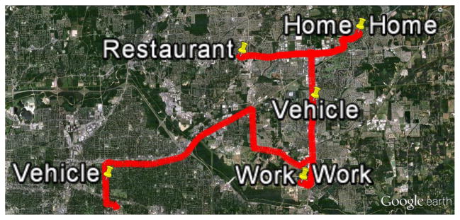
A sample GPS trace for one day from a participant. The red line shows the path commuted by the participant. The pinned locations are the location at the time of EMA prompt.

Label assignment is based on demographic, temporal and business features. Demographic features include the age and gender of the participant, which are obtained from recruitment forms. The temporal features include the arrival time, visit midpoint time, departure time, season, holiday, and the duration of stay at that location. These features were computed from the GPS traces and clusters. Lastly, the business features include the count of different types of business entities such as Arts/Entertainment, Food/Dining, Government/community, Education, etc. within different distance thresholds from the current location (see [27] for details). To compute the business features, we used Google Places API. For this model, we obtain an accuracy of 85.8% (and κ = 0.80). Table 1 presents the confusion matrix for this semantic context labeler model where F-measure is 0.85 and area under the curve is 0.97. We observe that Home, Work, and Store are detected quite well. But, Restaurant is confused with Store, because a Store and a Restaurant can be co-located. We correct the labels (if necessary) by plotting the GPS traces in Google earth and by visually inspecting it. These location labels were considered as ground truth. But, in some cases we could not reliably distinguish between a store and a restaurant (due to inherent GPS inaccuracy). We discard these data points by marking them unknown.

Table 1.

Confusion Matrix for the Semantic Labeling model [27].

	Classified as
	Home	Work	Store	Restaurant	Other
Home	617	11	10	0	4
Work	12	708	1	0	1
Store	8	7	203	6	9
Restaurant	4	1	43	27	3
Other	62	14	40	1	96

We also obtain a detailed level of semantic labeling. For Home, detailed label can be Indoor Home, Dormitory, and Backyard. Figure 2 shows a detailed breakdown of the labels. Our labeling concept of these details evolved over time [28] (e.g., by adding new levels). Hence, we made multiple iterations to obtain consistent labels.

Figure 2.

Two level semantic labeling of GPS clusters.

Driving Detection

Driving is detected from GPS-derived speed and by applying a threshold for maximum gait speed of 2.533 meters/sec [9]. A driving session is composed of driving segments separated by stops, e.g., due to a traffic light being red. Stops usually are of short duration unless there is a congestion. The end of a driving session is defined as a stop (speed=0) for more than 2 minutes. Otherwise, two driving segments sandwiched by a less than 2 minute stop is considered to be part of the same driving session. In case of loss of GPS signal for more than 30 seconds we also end the driving session at the timestamp when we received the last GPS sample. In order to determine whether participant is driving or just riding a vehicle we use the EMA question “If you commuted since the last interview, what type?”, where possible responses are “Driving”, “Biking”, “Walking”, “Riding as a Passenger”, “Riding Public Transportation”, and “Did not commute”. Finally, if an EMA prompting time is between start and end of a driving session, and the self-report response mentions “Driving”, we mark that EMA to occur during driving.

Activity Inference

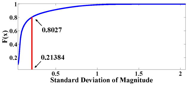
To infer whether a subject is in motion or not, we use a simple threshold based activity detector using the 3-axis on-body accelerometer (placed on chest). Phone accelerometer data was not used because the phone may not be on the person and thus may miss some physical activity. We adapt the physical movement detection approach in [3,39]. As the placement of the accelerometer and the participant population is different from that presented in prior works, we collected training data to determine an appropriate threshold for detecting activity. We collected labeled data under walking and running (354.16 minutes), and stationary (1426.50 minutes) states from seven pilot participants who wore the same sensor suite. Figure 3 shows the training data from seven pilot participants. We filtered the raw signal, removed the drift, and extracted the standard deviation of magnitude, which is independent of the orientation of the accelerometers and recommended in literature [3, 39]. We find the distinguishing threshold for our accelerometer to be 0.21384, which is able to distinguish stationary from non-stationary states with an accuracy of 97% in 10-fold cross-validation. Figure 4 shows that subjects were physically active for around 20% of their total wearing time.

Figure 3.

Standard deviations < 0.21384 are labeled as stationary and others are labeled as non-stationary (i.e., walking or running).

Figure 4.

Using cut-off point 0.21384 we observe that subjects were physically active for around 20% of their total wearing time.

Stress Inference

Measurements from the ECG and RIP sensors were used to extract 13 features (including heart rate variability) for physiological stress model as proposed in [40]. The model produces binary outputs on 30 second segments of measurements that indicate whether a person is stressed or not. A correlation of 0.71 between the stress model and the self-reported rating of stress was reported in [40] in both lab and 2-day field study with 21 participants. As proposed in [40], stress inference is discarded when the participant is not stationary.

METRIC FOR MEASURING AVAILABILITY

We define availability as a state of an individual in which (s)he is capable of engaging in an incoming, unplanned activity. For example, consider a software engineer who has just quit smoking, is working on a project, when (s)he receives a JITI on the mobile phone, perhaps triggered by an acute stress detection from sensors. In response, (s)he could − 1) stop ongoing work and engage in the intervention (e.g., do a biofeedback exercise to relax), 2) continue working on the project for a short time (pre-specified threshold) and then stop the work to engage in JITI, 3) continue working on the project but attend to JITI later, or 4) completely ignore the JITI. In our proposed definition, for cases 1 and 2 the software engineer will be considered as available while for cases 3 and 4 (s)he will be considered unavailable. We first consider delay in starting to answer a randomly prompted EMA as a metric for measuring availability.

Response Delay

Response delay for an EMA is the duration between the prompt time and the time of completion of the first item in the EMA. Figure 5 shows the probability distribution of response delay across all participants. Delay distribution fits a Gamma distribution with shape parameter κ = 1.2669 and scale parameter θ = 35.5021. We use the p = 0.95 cutoff (which occurs at 124 seconds) as the grace period to obtain a good separation between the available and unavailable states.

Figure 5.

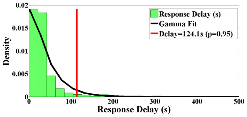
Delay distribution is fitted with a Gamma distribution with shape parameter κ =1.2669 and scale parameter θ =35.5021. We use the cutoff of p = 0.95 that occurs at 124.1 seconds, as the grace period. A response delay beyond this grace period is marked as unavailable.

Since each EMA is associated with a micro-incentive, it is plausible that some participants may be financially sensitive and fill out each EMA in a timely fashion, even when not fully available. In such cases, they may complete some EMA’s quickly without sufficient care. We, therefore, consider completion time as another metric to complement response delay.

Completion Time

Completion Time for an EMA is the ratio of total completion time to the number of items answered. However, time to answer the first item includes the time to take the phone out. Therefore, we compute completion time, starting from the second item. Finally, there is between person difference in completion time due to participant’s cognitive processing, typing variations, and affinity to micro-incentive. To remove these biases, we compute the z-score of completion time for each participant and then use this z-score in further analysis.

To investigate if there is a threshold such that a completion time of lower than this threshold indicates urgency and lack of care in answering an EMA, we measure the consistency of response to the EMA. For this purpose, we use a measure of consistency that is used widely in psychometrics. It is called Cronbach’s alpha [8]. For a given set of items in an EMA (with numerical responses) that measure the same psychological construct, Cronbach’s alpha is given by

$$\alpha =\frac{k}{k-1}(1-\frac{\sum s_i^2}{\sum s_T^2}),$$

where k is the number of items in the set, $s_i^2$ is the variance in response to the i^th item, and $s_T^2$ is the variance of the total scores formed by summing up the responses to all the items in the set. We observe that if all the items in the set have equal variance and thus were perfectly correlated, we obtain α = 1. On the other hand, if all the items in the set are independent, α = 0. An α ≥ 0.7 is regarded as acceptable [8].

In our 42-item EMA, there are several affect items that measure the same psychological construct. These items are Cheerful?, Happy?, Energetic?, Frustrated/Angry?, Nervous/Stressed?, and Sad?, where participants respond on a Likert scale of 1–6. To compute alpha, items that assess positive affect (Cheerful, Happy, and Energetic) are retained as scored and items that assess negative affect (Frustrated/Angry, Nervous/Stressed, and Sad) are reverse coded (e.g., 1 becomes 6). To test whether these six items indeed measure the same psychological construct, we compute the overall alpha score for all responses from all participants. The overall α = 0.88 indicates a good agreement [16].

We next compute the Cronbach’s alpha score for various thresholds of (z-scores of) completion times. We observe that the 42-item EMA questionnaire contains different types of item. First, there are single choice items which participant can answer right away. Second, there are multiple choice items which requires going through various possible answers, which may take more time. Third, there are recall based items where participants need to remember about past actions. An example of such an item is “How long ago was your last conversation?”. Such items may require longer to complete. We consider subsets of EMA items in each of the above three categories and compute their corresponding z-scores. Figure 6 plots the alpha values for various thresholds on completion times for four cases — when the completion time for all items is considered and when the completion times for each of the above three subset of EMA items is considered. Since our goal is to find a lower threshold such that completing EMA items quicker than this threshold may indicate lack of availability, we only plot completion times lower than average (i.e., z-score of 0). We observe that in each case, α ≥ 0.7, which implies that completing EMA items quickly does not indicate inconsistent response. Hence, completion time is not a robust estimator of unavailability and we retain only the response delay as our metric of unavailability.

Figure 6.

We plot Cronbach’s alpha value for various thresholds of z-score of completion times. We observe that the alpha is always acceptable (i.e., ≥ 0.7). This holds even when we consider various subsets of items that require recollection or multiple choice selection.

Labeling of Available and Unavailable States

When an EMA prompt occurs, the phone beeps for 4 minutes. If the participant begins answering or presses the delay button, this sound goes away. There are 4 possible outcomes for each such prompt — i) Missing: Participant neither answers the EMA nor presses delay, i.e., just ignores it, ii) Delayed: Participant explicitly delays the EMA, and plans to answer it when (s)he becomes available, iii) After Grace: Participant answers after a grace period, which is defined in Figure 5, iv) Before Grace: Participant answers within the grace period. We mark the first three scenarios as Unavailable.

To identify available EMAs, we use two different approaches. In the first, we take n quickest answered EMA’s from each participant, where n is the number of EMA prompts when this participant was found to be unavailable. We mark each such EMA as available. We call this a Representative dataset, because it gives more weight to those participants’ data, who sometimes forego micro-incentives by missing or delaying EMA’s when they are not available. This may be similar to the situation in a class where several students may have a question, but only a few speak up, thus helping others who may be shy. This dataset gives less weight to data from those participants who are always prompt in answering EMA’s, due to their sincerity, scientific devotion to the study, or affinity to micro-incentives. This dataset thus recognizes and respects wide between person variability inherent in people.

Counting missed, delayed, or delayed above grace period (124.1s), we label 170 EMA’s as triggered when participants were unavailable. Number of instances when a participant was unavailable ranges from 0 to 15. By marking n quickest answered EMA from each participant as available, where n is the number of EMA prompts for which that particular participant was unavailable, we obtain a total of 340 EMA’s for training data. This dataset provides a robust separation of delay between the available and unavailable class (with a mean of 141.4s±51.7s and a minimum separation of 107.7s). This kind of wide separation helps us mitigate the effect of delay in taking out the phone to answer an EMA.

Due to the definition of Representative dataset, 3 participants are completely ignored due to always being compliant, responding within grace period, and never delaying an EMA. Hence, we construct a Democratic dataset, where we consider equal number of EMA’s from each participant. To obtain a similar size of training data as in the Representative dataset, we use 6 quickest EMA from each participant as available and 6 slowest (including delayed or missed) as unavailable. We thus obtain 12 samples from each participant, making for a total of 360 samples. The delay separation between available and unavailable class in this dataset has a similar mean of 169.8s, but a higher standard deviation of 193.8s, and a smaller minimum separation of 5.2s.

FINDINGS

Before presenting our model for predicting availability, we conduct a preliminary analysis of various factors in this section to understand their role in predicting availability. We investigate various contextual factors (e.g., location, time, etc.), temporal factors (e.g., weekend vs. weekdays, time of transition, etc.), mental state (e.g., happy, stressed, etc.), and activity state (e.g., walking, driving, etc.).

Figures 7 and 8 present the probability of participants being available and the mean response delay across different contexts (e.g., location, activity, mental state, and time) respectively. In these figures, outside refers to outside of home, work, store, restaurant, and vehicle. We observe in Figure 8 that the response delay has high variance (range 23.2–137.5) across different contexts, which can be attributed to the Gamma distribution of response delay (see Figure 5).

Figure 7.

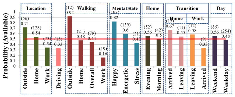
Probability of participants being available across different contexts. Here morning is defined as before 9 AM and evening as after 5 PM. Arrived at a location means arrival within 30 minute, while leaving means 30 minute prior to leaving. Red line is drawn for p(A) = 0.5.

Figure 8.

Mean response delay across different contexts. Morning, evening, arrival, and leaving are defined as in Figure 7. Red line represents the overall mean of 49.5s (±116.0s).

Location

From Figure 7, we observe that participants are more likely to be available (p(A) = 0.71¹) when they are outside and they are most likely to be unavailable at work (p(A) = 0.34). When participants are outside, their response delay is also lower than any other location (mean=41.0s; p = 0.074 on Wilcoxon rank-sum) (see Figure 8). This lower response delay may be because when participants are outside, they are unlikely to be engaged in a time-sensitive activity (e.g., deadline, driving a vehicle) and thus can attend to the incoming prompt relatively quickly. As expected, during driving participants are usually unavailable (p(A) = 0.33) and the delay in response during driving is significantly higher than other times (p = 0.019 on Wilcoxon rank-sum).

Walking

In contrast to [20], which found posture change as an indication of being interruptible, we find that in daily life, walking by itself does not indicate availability (p(A) = 0.44). Interestingly though, walking outside indicates a highly available state (p(A) = 0.92), while walking at work indicates a highly unavailable state (p(A) = 0.16). We observe a mean response delay of 29.7s when participants are walking outside, which is not significantly lower than stationary (p = 0.318 on Wilcoxon rank-sum), but significantly lower (p = 0.008 on Wilcoxon rank-sum) when compared with other locations (e.g., home, work, etc.).

Mental State

When participants are in a happier state, they are more likely to be available (p(A) = 0.82) and we observe a lower response delay (mean=41.3s; p = 0.008 on Wilcoxon rank-sum). Similarly, when participants are feeling energetic, they are more available (p(A) = 0.6). But, unlike happy, in the energetic state the delay (45.2s) decrease is not significant (p = 0.144 on Wilcoxon rank-sum). On the other hand, participants being stressed reduces the probability of being available (p(A) = 0.43). A good news for JITI that may be triggered upon detection of stress is that participants are not found to be highly unavailable when stressed as is the case at work. Such JITI, therefore, may still be attended to by users. Investigation of the receptivity of stress-triggered JITI may represent an interesting future research opportunity.

Home

Since being at home indicates only a marginally available state (p(A) = 0.54), we investigate whether time of day makes a difference. We find that availability at home is lower during morning (p(A) = 0.5), and higher in the evening (p(A) = 0.56), but not by much. However, response delay in the morning (54.5s) is higher than that in the evening (41.8s) (p = 0.052 on Wilcoxon rank-sum). This indicates that participants are more pressed for time in the morning.

Transition

To further investigate the effect of location on availability, we analyze the availability of participants when they are about to leave a place (within 30 minutes of departure) or have just arrived at a place (30 minute since arrival). We find that the availability of participants when leaving home (p(A) = 0.55) is similar to when in home generally. But, their availability is higher when they have just arrived home (p(A) = 0.67). The scenario is reversed at work. The availability at work upon arrival (p(A) = 0.33) is similar to the overall availability at work. But, their availability is higher when about to leave work (p(A) = 0.58).

Day

Finally, we analyze the effect of weekday vs. weekend. We find that participants are more likely to be available on weekend (p(A) = 0.56) than on weekdays (p(A) = 0.48). Interestingly, the response delay on weekends is higher than that during weekdays (p = 0.061 on Wilcoxon rank-sum).

Although one could investigate several combinations of factors, we next develop a model that uses several features derived from these factors to predict availability of participants.

PREDICTING AVAILABILITY

In this section, we develop a model to predict availability. We first discuss the features we compute, feature selection methods to find the most discriminating features, and then the machine learning model to predict availability. We conclude this section by reporting the evaluation of our availability model.

Feature Computation

To predict availability, we compute a variety of features. Majority of them come from sensors, but we also obtain several from self-reported EMA responses because the sensor models for their detection is not mature enough today to detect them with reasonable confidence. We expect that these features will also become reliably detectable from sensors in near future. In total, we compute 99 features.

Clock: Time and Day (6 features)

We compute several time related features. We include “day of the week” since there may be a day-specific influence, “elapsed hour” in a day to identify work vs. non-work hours, and “Time since last EMA” to capture the cumulative fatigue caused by frequent EMA prompts. We also include binary features such as “Working Hour?”, which is defined to be between 9 AM and 5 PM, “Weekend?”, and “Holiday?”.

Sensor: Stress (4+24 features)

As discussed earlier, we infer stress level for each 30 second window. Since sometimes EMA prompts itself may cause stress, we used binary stress levels in the 30 second windows prior to the generation of an EMA prompt. From these windows, 24 derived features are computed (see Table 2), similar to that in [13]. We note that if the participant is physically active during a 30-second window, we mark the stress feature as undefined for this window (due to stress being confounded by physical activity). Hence, stress level in each of the 30 second windows for derived features may not be available. Consequently, we compute four other features. The first two of these come from the first window preceding the prompt where stress inference is available (i.e., unaffected by physical activity). Binary stress state and probability of being stressed are used as features from this first window. The remaining two features are the number of windows where the participant is stressed over the prior 3 (and 5) windows preceding the prompt, for which stress inference is available. These windows must occur within 5 minutes prior to the prompt.

Table 2.

For 6 values of N (30 seconds, 1 min, 2 min, 3 min, 4 min, and 5 min), the above four derivative features are computed for stress and activity, producing 24 features for each.

All-N	Event occurred in every past window within N second of corresponding sensor prior to random EMA prompt
Any-N	Event occurred in any past window within N second of corresponding sensor prior to random EMA prompt
Duration-N	Duration of occurrence of event within past N second prior to EMA prompt
Change-N	Number of change where event occurred in one window followed by non-event within N second prior to EMA prompt

Sensor: Location, Place, Commute Status (7 features)

We compute several location related features. This includes coarse level location such as Home, Work, Store, Restaurant, Vehicle, and Other and detailed location such as inside home, dormitory, backyard, etc. We also include “Previous Location” and “time spent in current location” because it is likely that after immediate arrival at home from work or from other locations people are less likely to be available. We include a binary feature for “driving” because driving requires uninterrupted attention and distraction during driving can result in injury, loss of life, and/or property. It is also illegal in several parts of the world to engage a driver in a secondary task such as texting. Since EMA prompts are generated randomly (as per the norm in behavioral science [48]), some EMA prompts did occur during driving. Participants were instructed to find a safe place to park the car in such cases before answering. A binary feature outdoor is also included since we observe participants being more available when they are outdoors and walking.

Sensor: Physical Activity (3+24 features)

Since physical activity can also indicate availability, we use physical activity data from the chest accelerometer sensor as a binary feature, and intensity of activity as a numeric feature. EMA questionnaire contains items such as “Describe physical movement” with possible answers “Limited (writing)”, “Light (walking)”, “Moderate (jogging)”, and “Heavy (running)”. We include features such as writing as a categorical feature because writing state may affect availability and we are unable to infer it activities from our sensors with reasonable confidence today.

EMA: Activity Context (13 features)

EMA questionnaire asked participants to describe their ongoing activity using the following items: “How would you describe your current activity?”, with possible responses as “Leisure/Recreation” or “Work/Task/Errand”, a multiple choice item “What’s going on?” with possible responses as Meeting, E-mail, Reading, Phone Call, Writing, Sports, Video Game, Surfing the Internet, Watching Movies/TV/Video, Listening to Music, and Other. Each possible response is used as a binary feature. We also use binary response to the “Taken alcohol?” item.

EMA: Social Interaction (6 features)

Research on interruption has revealed that situations involving social engagement are considered less interruptible [6, 15, 18]. To model availability, we used participants’ responses for the social interaction related EMA queries that includes “In social interaction?”, “Talking?”, “If talking, on the phone?”, “If talking, with whom?”, “If not talking, how long ago was your last conversation?”, and “Who was it with?”.

EMA: Mental State (9 features)

We also include emotional state due to their wide acceptability as a factor in Human Computer Interaction [7, 26]. Although stress is detectable from sensors, affect is not yet detectable reliably in the field setting from physiological sensors. Hence, we use EMA responses. We include response to our EMA items, “Cheerful?”, “Happy?”, “Frustrated/Angry?”, “Nervous/Stressed?”, “Sad?”, “Facing a problem?”, “Thinking about things that upset you?”, “Difficulties seem to be piling up?”, and “Able to control important things?”. Response in Likert scale 1–6 is used as feature.

EMA: Fatigue (3 features)

Each EMA prompt resulted in some level of fatigue on the recipient [23]. We find that responses to the first half of the EMA’s are more consistent than the second half EMA for the day (p = 0.056, n = 30, paired t-test on Cronbach’s alpha). Therefore, we add EMA index of the day as a feature. Our EMA questionnaire contained items such as “Energetic?” and “Sleepy?”. Subjective responses of these items in 1–6 Likert scale are also used as features.

Feature Selection

As reported in the preceding, a total of 99 features were computed. But, to avoid overfitting of the model, we select a subset of the features for modeling availability. We base our feature selection on two complementary methods.

Correlation based Feature Subset Selection

Our goal is to find features that are highly correlated to the class available vs. unavailable, and not correlated with each other. We used Hall’s [17] method to find the optimal non-correlated feature set regardless of the underlying machine learning algorithm.

Wrapper for Feature Subset Selection

Correlation based feature selection may discard some features that are useful for a particular machine learning algorithm. Therefore, we also use Wrapper [25] based feature selection to find an optimal feature subset for the SVM machine learning algorithm [41].

By taking a union over the features selected by correlation based feature selection and Wrapper applied to SVM, we obtain a total of 30 features. Table 3 lists these features ordered according to their information gain [11]. We make several observations. First, we observe that most of the features selected are either already detectable from sensors (1–4, 8, 11–30) or are potentially detectable in near future from sensors (9–10). But, three features (5–7) are hard to detect automatically today. An inward looking camera in smart eyeglasses could potentially detect some of these in near future as well. Second, we observe that stress features (16–19, 21–26) figure quite prominently in this list, indicating a significant role of stress in predicting availability. Finally, we observe that driving is not included in the list of selected features, though intuitively it appears relevant. We hypothesize that features ranked 1, 2, 4, and 8 contain information about driving and as such driving may not be needed as a separate feature.

Table 3.

Selected 30 features ranked (R) according to information gain. Detailed location offers the highest information gain.

R	Feature
1	Detailed Location
2	Coarse Location
3	Weekday
4	Outdoor?
5	Sleepy?
6	Happy?
7	Energetic?
8	Commute Mode?
9	Recreation?
10	Activity type
11	Weekend?
12	Talking on phone?
13	Taken Alcohol?
14	Elapsed hour of day
15	Time spent in current location
16	Stress probability
17	Stress count in 5 previous window
18	StressChange-300
19	StressChange-240
20	ActivityAll-120
21	StressAny-180
22	StressChange-180
23	StressAny-240
24	StressAny-60
25	StressChange-30
26	StressDuration-30
27	ActivityAll-180
28	ActivityAll-240
29	ActivityAny-300
30	EMA Index

Model

Due to its well-accepted robustness, we train a Support Vector Machine (SVM) [41] model with RBF kernel to predict availability of users. To evaluate the model, we use both the standard 10 fold cross-validation and leave-one-subject-out to evaluate between subject generalizability. As described earlier, we use two diverse methods to label EMA’s as available and unavailable to generate training data. We present the performance of the model on each of these labeling methods.

Representative Dataset

Based on the missed, explicitly delayed, or delayed above grace period (124.1s) we mark 170 EMA’s as triggered when participants were unavailable. We mark the n quickest answered EMA from each participant as available, where n is the number of EMA prompts for which that particular participant was unavailable. This provides us with 340 instances as training data for modeling with 170 instances coming from each class².

Using this dataset we get an overall accuracy of 74.7% (against a base accuracy of 50%) with kappa of 0.494 for 10-fold cross-validation. From the confusion matrix in Table 4, we find that for 78.8% cases, the classifier is able to predict availability versus 70.6% in the case of unavailability. We get a precision of 0.749, a recall of 0.747, an F-measure of 0.747, and area under the curve of 0.747. For leave-one-subject-out, we get a weighted average accuracy of 77.9%.

Table 4.

Confusion Matrix for predicting availability using SVM model on RBF kernel built on Representative Dataset. Overall Accuracy is 74.7% against a base accuracy of 50%, with a kappa of 0.494.

	SVM Classified as
	Available	Unavailable
Available	134 (78.8%)	36 (21.2%)
Unavailable	50 (29.4%)	120 (70.6%)

Democratic Dataset

In this dataset, we take 12 samples from each participant, which leads to similar 360 samples from 30 participants. The 6 quickest responded EMA’s are considered available and 6 slowest responded ones (including explicitly delayed ones) are considered as unavailable.

For this labeling, the SVM model achieves an accuracy of 69.2% with a kappa of 0.383, slightly lower than the Representative model. However, from the confusion matrix in Table 5, we find that for 75.0% cases, classifier is able to predict availability. We get a precision of 0.694, a recall of 0.692, an F-measure of 0.691, and area under the curve of 0.692. For leave-one-subject-out, we get an accuracy of 76.4%.

Table 5.

Confusion Matrix for predicting availability using SVM model on RBF kernel built on Democratic Dataset. Overall Accuracy is 69.2% against a base accuracy of 50%, with a kappa of 0.383.

	SVM Classified as
	Available	Unavailable
Available	135 (75.0%)	45 (25.0%)
Unavailable	66 (36.7%)	114 (63.3%)

LIMITATIONS AND FUTURE WORK

Being the first work to inform the timing of sensor-triggered just-in-time intervention (JITI), this work has several limitations that open up interesting opportunities for future works. First, several features used to predict availability are not yet reliably detectable via sensors today. For a model to be automated in informing the timing of JITI, all features need to be inferred from sensors. Second, this work used data from wearable sensors. Since wearing sensors involves user burden, it is more desirable to use only those sensors that are available on the phone. But, some features are not feasible to obtain today from phone sensors (e.g., stress) and hence represents interesting future works. Third, the type of sensors available on the phone is growing richer rapidly. Several sensors such as proximity sensor, acoustic sensor, and phone orientation and other data in the phone (e.g., calendar, task being performed on the phone, etc.) that may inform the current context of a user were not used in this work. Using these and other sensors emerging in phone may further improve the prediction accuracy. Similarly, using additional sensors on the body and those in instrumented spaces such as office, home, and vehicle (e.g., cameras) can also be used wherever available to further improve the prediction accuracy.

Fourth, this work used micro-incentive to improve compliance in responding to EMA prompts and used it to accomplish a high level of motivation. Although the work presented in this paper can inform the timing of delivering randomly prompted self-reports in scientific studies, it remains an open question how well the micro-incentive captures the motivation level expected in users who choose to use JITI due to certain health condition or due to a wellness or fitness motivation.

Fifth, given that filling out a 42-item EMA requires significant user involvement (i.e., 2.4 minutes to complete), the results of this work may be more applicable to JITI that involve similar engagement. Its applicability to lighter JITI may need further investigation. We note, however, that if the user is found to be unavailable for a more involved active JITI (e.g., when driving), passive intervention could be delivered in the meantime (e.g., by playing music [37]).

Sixth, the analysis in this work used only the unanticipated (i.e., randomly prompted) EMA’s to simulate the triggering of a sensor-triggered JITI, but the participants also filled out EMA’s that resulted from their self-initiation. Although these self-initiated EMA’s were voluntary, they may add to the burden and fatigue of participants. It remains open whether the results of a future study that only uses randomly prompted EMA’s may be any different than the one reported here.

CONCLUSION

Sensor-triggered just-in-time-interventions (JITI) promise to promote and maintain healthy behavior. But, critical to the success of JITI is determining the availability of the user to engage in the triggered JITI. This paper takes a first step to inform the timing of delivering JITI. We propose a novel objective metric to measure a user’s availability to engage in a JITI and propose a model to predict availability in the natural environment based on data collected in real-life. Our findings indicate that availability of a user depends not only on user’s ongoing activity or physical state, but also on user’s psychological state. Our results can inform the design of JITIs and opens up numerous opportunities for future works to improve the accuracy, utility, and generalizability of our model.

References

- 1.al Absi M, Hatsukami D, Davis G, Wittmers L. Prospective examination of effects of smoking abstinence on cortisol and withdrawal symptoms as predictors of early smoking relapse. Drug and alcohol dependence. 2004;73(3):267–278. doi: 10.1016/j.drugalcdep.2003.10.014. [DOI] [PubMed] [Google Scholar]
- 2.Alpers G. Ambulatory assessment in panic disorder and specific phobia. Psychological Assessment. 2009;21(4):476. doi: 10.1037/a0017489. [DOI] [PubMed] [Google Scholar]
- 3.Atallah L, Lo B, King R, Yang G. Sensor placement for activity detection using wearable accelerometers. Body Sensor Networks (BSN) 2010:24–29. [Google Scholar]
- 4.Avrahami D, Fogarty J, Hudson S. Biases in human estimation of interruptibility: effects and implications for practice. ACM CHI. 2007:50–60. [Google Scholar]
- 5.Avrahami D, Gergle D, Hudson S, Kiesler S. Improving the match between callers and receivers: A study on the effect of contextual information on cell phone interruptions. Behaviour & Information Technology. 2007;26(3):247–259. [Google Scholar]
- 6.Bangerter A, Chevalley E, Derouwaux S. Managing third-party interruptions in conversations: Effects of duration and conversational role. Journal of Language and Social Psychology. 2010;29(2):235–244. [Google Scholar]
- 7.Bessiere K, Newhagen J, Robinson J, Shneiderman B. A model for computer frustration: The role of instrumental and dispositional factors on incident, session, and post-session frustration and mood. Computers in human behavior. 2006;22(6):941–961. [Google Scholar]
- 8.Bland J, Altman D. Statistics : notes cronbach’s alpha. BMJ. 1997;314(7080):572–572. doi: 10.1136/bmj.314.7080.572. [DOI] [PMC free article] [PubMed] [Google Scholar]
- 9.Bohannon R. Comfortable and maximum walking speed of adults aged 20–79 years: Reference values and determinants. Age and ageing. 1997;26(1):15–19. doi: 10.1093/ageing/26.1.15. [DOI] [PubMed] [Google Scholar]
- 10.Burns M, Begale M, Duffecy J, Gergle D. Harnessing context sensing to develop a mobile intervention for depression. Journal of medical Internet research. 2011;13(3) doi: 10.2196/jmir.1838. [DOI] [PMC free article] [PubMed] [Google Scholar]
- 11.Cover TM, Thomas JA. Elements of information theory. John Wiley & Sons; 2012. [Google Scholar]
- 12.Fisher R, Simmons R. Smartphone interruptibility using density-weighted uncertainty sampling with reinforcement learning. IEEE ICMLA. 2011;1:436–441. [Google Scholar]
- 13.Fogarty J, Hudson S, Atkeson C, Avrahami D, Forlizzi J, Kiesler S, Lee J, Yang J. Predicting human interruptibility with sensors. ACM TOCHI. 2005;12(1):119–146. [Google Scholar]
- 14.Fogarty J, Hudson S, Lai J. Examining the robustness of sensor-based statistical models of human interruptibility. ACM CHI. 2004:207–214. [Google Scholar]
- 15.Fonner KL, Roloff ME. Testing the connectivity paradox: Linking teleworkers’ communication media use to social presence, stress from interruptions, and organizational identification. Communication Monographs. 2012;79(2):205–231. [Google Scholar]
- 16.George D, Mallery M. Using spss for windows step by step: a simple guide and reference. 2003. [Google Scholar]
- 17.Hall MA. PhD thesis. University of Waikato; Hamilton, New Zealand: 1998. Correlation-based Feature Subset Selection for Machine Learning. [Google Scholar]
- 18.Harr R, Kaptelinin V. Interrupting or not: exploring the effect of social context on interrupters’ decision making. ACM NordiCHI. 2012:707–710. [Google Scholar]
- 19.Hayes T, Cobbinah K, Dishongh T, Kaye J, Kimel J, Labhard M, Leen T. A study of medication-taking and unobtrusive, intelligent reminding. Telemedicine and e-Health. 2009;15(8):770–776. doi: 10.1089/tmj.2009.0033. [DOI] [PMC free article] [PubMed] [Google Scholar]
- 20.Ho J, Intille S. Using context-aware computing to reduce the perceived burden of interruptions from mobile devices. ACM CHI. 2005:909–918. [Google Scholar]
- 21.Hudson S, Fogarty J, Atkeson C, Avrahami D, Forlizzi J, Kiesler S, Lee J, Yang J. Predicting human interruptibility with sensors: a wizard of oz feasibility study. ACM CHI. 2003:257–264. [Google Scholar]
- 22.Iqbal S, Bailey B. Effects of intelligent notification management on users and their tasks. ACM CHI. 2008:93–102. [Google Scholar]
- 23.Kapoor A, Horvitz E. Experience sampling for building predictive user models: a comparative study. ACM CHI. 2008:657–666. [Google Scholar]
- 24.Kaushik P. PhD thesis. Massachusetts Institute of Technology; 2005. The design and evaluation of a mobile handheld intervention for providing context-sensitive medication reminders. [Google Scholar]
- 25.Kohavi R, John GH. Wrappers for feature subset selection. Artificial Intelligence. 1997;97(1–2):273–324. Special issue on relevance. [Google Scholar]
- 26.Krediet I. PhD thesis. Tilburg University; 1999. Work and Emotions: The Role of Interruptions. [Google Scholar]
- 27.Krumm J, Rouhana D. Placer: Semantic place labels from diary data. ACM UbiComp. 2013:163–172. [Google Scholar]
- 28.Kulesza T, Amershi S, Caruana R, Fisher D, Charles D. Structured labeling for facilitating concept evolution in machine learning. ACM CHI. 2014:3075–3084. [Google Scholar]
- 29.Kumar S, Nilson W, Pavel M, Srivastava M. Mobile health: Revolutionizing healthcare through trans-disciplinary research. IEEE Computer. 2013;46(1):28–35. [Google Scholar]
- 30.Marije R, Hogenelst K, Schoevers R. Mood disorders in everyday life: A systematic review of experience sampling and ecological momentary assessment studies. Clinical Psychology Review. 2012;32(6):510–523. doi: 10.1016/j.cpr.2012.05.007. [DOI] [PubMed] [Google Scholar]
- 31.Mark G, Gudith D, Klocke U. The cost of interrupted work: more speed and stress. ACM CHI. 2008:107–110. [Google Scholar]
- 32.McFarlane D. Comparison of four primary methods for coordinating the interruption of people in human-computer interaction. Human-Computer Interaction. 2002;17(1):63–139. [Google Scholar]
- 33.Minami H, McCarthy D, Jorenby D, Baker T. An ecological momentary assessment analysis of relations among coping, affect and smoking during a quit attempt. Addiction. 2011;106(3):641–650. doi: 10.1111/j.1360-0443.2010.03243.x. [DOI] [PMC free article] [PubMed] [Google Scholar]
- 34.Mokdad AH, Marks JS, Stroup DF, Gerberding JL. Actual causes of ddeath in the united states, 2000. Journal of the American Medical Association (JAMA) 2004;291(10):1238–1245. doi: 10.1001/jama.291.10.1238. [DOI] [PubMed] [Google Scholar]
- 35.Montoliu R, Blom J, Gatica-Perez D. Discovering places of interest in everyday life from smartphone data. Multimedia Tools and Applications. 2013;62(1):179–207. [Google Scholar]
- 36.Musthag M, Raij A, Ganesan D, Kumar S, Shiffman S. Exploring micro-incentive strategies for participant compensation in high-burden studies. ACM UbiComp. 2011:435–444. [Google Scholar]
- 37.Nirjon S, Dickerson R, Li Q, Asare P, Stankovic J, Hong D, Zhang B, Jiang X, Shen G, Zhao F. Musicalheart: A hearty way of listening to music. ACM SenSys. 2012:43–56. [Google Scholar]
- 38.Oorschot M, Kwapil T, Delespaul P, Myin-Germeys I. Momentary assessment research in psychosis. Psychological assessment. 2009;21(4):498–505. doi: 10.1037/a0017077. [DOI] [PubMed] [Google Scholar]
- 39.Pandian P, Mohanavelu K, Safeer K, Kotresh T, Shakunthala D, Gopal P, Padaki V. Smart vest: Wearable multi-parameter remote physiological monitoring system. Medical engineering & physics. 2008;30(4):466–477. doi: 10.1016/j.medengphy.2007.05.014. [DOI] [PubMed] [Google Scholar]
- 40.Plarre K, Raij A, Hossain S, Ali A, Nakajima M, Al’absi M, Ertin E, Kamarck T, Kumar S, Scott M, et al. Continuous inference of psychological stress from sensory measurements collected in the natural environment. IEEE IPSN. 2011:97–108. [Google Scholar]
- 41.Platt J. Fast training of support vector machines using sequential minimal optimization. In: Schoelkopf B, Burges C, Smola A, editors. Advances in Kernel Methods - Support Vector Learning. MIT Press; 1998. [Google Scholar]
- 42.Poppinga B, Heuten W, Boll S. Sensor-based identification of opportune moments for triggering notifications. IEEE Pervasive Computing. 2014;13(1):22–29. [Google Scholar]
- 43.Preuveneers D, Berbers Y. Mobile phones assisting with health self-care: a diabetes case study. ACM MobileHCI. 2008:177–186. [Google Scholar]
- 44.Sadler K, Robertson T, Kan M. It’s always there, it’s always on: Australian freelancer’s management of availability using mobile technologies. ACM MobileHCI. 2006:49–52. [Google Scholar]
- 45.Serre F, Fatseas M, Debrabant R, Alexandre J, Auriacombe M, Swendsen J. Ecological momentary assessment in alcohol, tobacco, cannabis and opiate dependence: A comparison of feasibility and validity. Drug and alcohol dependence. 2012;126(1):118–123. doi: 10.1016/j.drugalcdep.2012.04.025. [DOI] [PubMed] [Google Scholar]
- 46.Shiffman S. Ecological momentary assessment (ema) in studies of substance use. Psychological Assessment. 2009;21(4):486. doi: 10.1037/a0017074. [DOI] [PMC free article] [PubMed] [Google Scholar]
- 47.Shiffman S, Paty JA, Gnys M, Kassel JA, Hickcox M. First lapses to smoking: Within-subjects analysis of real-time reports. Journal of Consulting and Clinical Psychology. 1996;64(2):366. doi: 10.1037//0022-006x.64.2.366. [DOI] [PubMed] [Google Scholar]
- 48.Shiffman S, Stone A, Hufford M. Ecological momentary assessment. Annu Rev Clin Psychol. 2008;4:1–32. doi: 10.1146/annurev.clinpsy.3.022806.091415. [DOI] [PubMed] [Google Scholar]
- 49.Stone A, Broderick J. Real-time data collection for pain: Appraisal and current status. Pain Medicine. 2007;8(s3):S85–S93. doi: 10.1111/j.1526-4637.2007.00372.x. [DOI] [PubMed] [Google Scholar]
- 50.Wenze SJ, Miller IW. Use of ecological momentary assessment in mood disorders research. Clinical psychology review. 2010;30(6):794–804. doi: 10.1016/j.cpr.2010.06.007. [DOI] [PubMed] [Google Scholar]