A Quantitative Measure of Field Illumination

Abstract

In this paper, we describe a statistically based algorithm to quantify the uniformity of illumination in an optical light microscopy imaging system that outputs a single quality factor (QF) score. The importance of homogeneous field illumination in quantitative light microscopy is well understood and often checked. However, there is currently no standard automatic quantitative measure of the uniformity of the field illumination. Images from 89 different laser-scanning confocal microscopes (LSCMs), which were collected as part of an international study on microscope quality assessment, were used as a “training” set to build the algorithm. To validate the algorithm and verify its robustness, images from 33 additional microscopes, including LSCM and wide-field (WF) microscopes, were used. The statistical paradigm used for developing the quality scoring scale was a regression approach to supervised learning. Three intensity profiles across each image—2 corner-to-corner diagonals and a center horizontal—were used to generate pixel-intensity data. All of the lines passed through the center of the image. The intensity profile data then were converted into a single-field illumination QF score in the range of 0–100, with 0 having extreme variation, and therefore, essentially unusable, and 100 having no deviation, i.e., straight lines with a constant uniform intensity. Empirically, a QF ≥ 83 was determined to be the minimum acceptable value based on manufacturer acceptance tests and reasonably achievable values. This new QF is an invaluable metric to ascertain objectively and easily the uniformity of illumination quality, provide a traceable reference for monitoring field uniformity over time, and make a direct comparison among different microscopes. The QF can also be used as an indicator of system failure and the need for alignment or service of the instrument.

Uniformity of illumination is one of the most crucial parameters in modern quantitative optical imaging. This is often referred to as the “flat field,” indicating that ideally all of the pixels in the image of a uniform sample would have the same brightness value across the field of view, i.e., flat.

Virtually, all of modern imaging and certainly all image quantization is based on “perfectly” even illumination. If there is variation within the field illumination, then all other parameters, such as illumination stability, coregistration, point spread function, etc., become mute.¹ Whereas an image with even illumination across the field of view would be ideal, current metrics of a maximum intensity variation of 10% along the image diagonal and 5% along the horizontal for the LSCMs were based on nominal microscope manufacturer acceptance criteria and routinely obtainable values. Therefore, published methods for measuring the uniformity of the image field of view do not offer a platform-independent, single quality metric or quality factor (QF).^2–4 This makes it difficult to track image illumination quality over time and nearly impossible to compare illumination quality between microscopes. Whereas the metric described here can be applied to any imaging platform that uses field illumination, for this paper, we concentrate on WF microscopes and LSCMs.

There are numerous components within the microscope that affect the level of homogeneity of the field illumination. The first is the uniformity of the illumination source. This is especially important when using mercury or xenon arc lamps on WF microscopes. These sources are based on a bulb that contains a central bright source of illumination (i.e., arc) that is inherently not uniform and requires some type of homogenization, such as a light diffuser or an optical scrambler. Most LSCMs use lasers as an illumination source, which are inherently coherent and uniform when they are functioning properly but are often coupled to the microscope that uses fiber optics. All illumination sources require some type of collection and relay optics to deliver the illumination light to the specimen. These intermediate optics introduce another source of nonuniformity in the field illumination. The problem of nonuniform illumination is widely recognized by microscopists as well as standards organizations, such as the American Society for Testing and Materials,⁵ as critical, especially as more quantitative data are extracted from light microscopy images and used to make scientific conclusions.⁶

MATERIALS AND METHODS

The field uniformity data that were used to develop the algorithm were collected as part of an international study and performance test of 89 different LSCMs and/or objective lenses from laboratories around the globe. The study was conducted by the Light Microscopy Research Group of the Association of Biomolecular Resource Facilities (ABRF). The details of the data collection have been published,⁷ but in brief, the protocol was as follows:

1. All lasers were warmed up for 1 h before imaging.

2. Images were collected within the coverslipped area of green or orange fluorescently doped plastic slides (Chroma Technology, Bellows Falls, VT, USA) by use of the 488 nm laser for excitation of the green slide or the 543 nm or the 561 nm laser for excitation of the orange slide.

3. Images were collected so that the intensity was ∼200 gray levels for 8-bit images.

4. The microscope zoom was set to the manufacturer’s specification (may not be 1).

5. Sufficient laser power was used so that the gain on the photomultiplier was ∼75% of the maximum value (typically, 500–600 V).

6. The intensity profile was measured across the image from 2 diagonal lines (upper left to lower right; upper right to lower left) and a center horizontal line drawn across the image.

The intensity profiles from the study data were used to train the computer algorithm method.

The algorithm was generated through training by use of data from the 89 microscopes from the international study. To validate the QF method, data from 33 WF microscopes or LSCMs were included in a reserved “confirmatory” dataset that were not used for the development of the QF score. The procedure used to collect these images was essentially the same as listed above. The 33 confirmatory microscopes were used to judge the robustness and validity of algorithm and the QF score (Table 1).

TABLE 1.

Microscope Type, Objective Lens, and Illumination Source

Microscope type	Sample size	Objective lens used	Illumination source
LSCMa	89a	20–15×a	Lasersa
LSCMb	15b	20×b	Lasersb
WFb	18b	10–20×b	Arc lampb

^aAlgorithm training set and ^bconfirmatory microscopes to validate the algorithm QF score determination.

Illumination Sources

The illumination and imaging techniques used in LSCM and WF microscopes are substantially different and are described below.

The most common illumination source used for the LSCM is a laser. The laser beam is scanned across the sample via a galvanometer mirror, with a fly-back from the end of one line to start the next line. As these microscopes have multiple lasers and pinholes, the coupling and alignment of the laser fiber optics to the scanning mirror are crucial to achieve uniform field illumination. The digital zoom capabilities of most LSCM make it possible to have even illumination (roll-off at the edges) across the entire field of view, typically at zoom ≥ 1.25. Therefore, most manufacturers will provide a specification, i.e., the expectable roll-off at the edges for a given zoom value. The specifications are typically 5% variation for the horizontal intensity across the center of the field of view and 10% for the intensity variation along the diagonal corner to corner of the field of view. The original acceptance test value should be consulted to determine what the exact values are. Whereas all of the confocal microscopes tested in this study were LSCM types, other types would also be amenable to these same tests, such as the spinning-disk confocal microscope. In principle, the algorithm and the QF determination are compatible with any intensity-based microscope image.

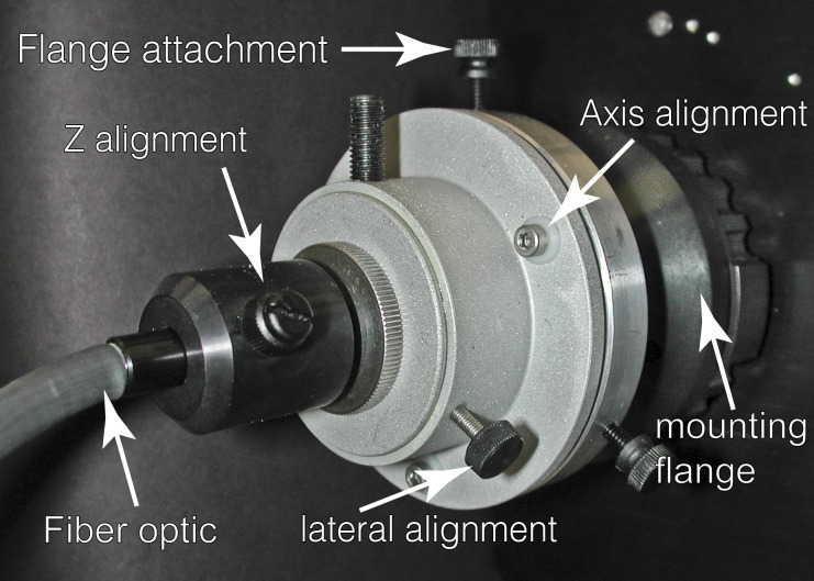
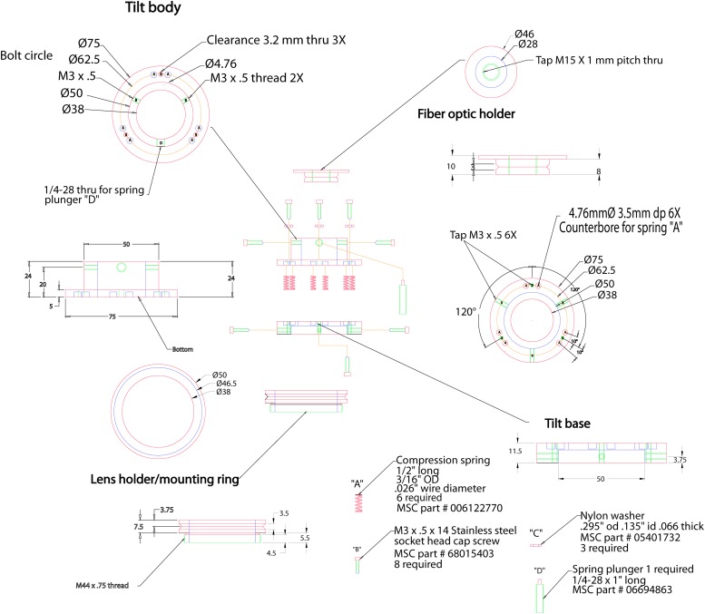
The illumination source for WF imaging is most commonly an external arc lamp coupled to the microscope, directly or with a fiber optic. However, light-emitting diode (LED) illumination sources are quickly replacing the traditional arc lamp. Similar to the arc lamp, LED light sources are also often coupled to the microscope via a fiber optic and coupling optics. The illumination must be delivered to the back aperture of the objective lens on axis to achieve even field illumination. Whereas tilted or off-axis illumination often goes undetected at high magnification, it can be problematic at lower magnification. The coupling of the fiber to the microscope often requires multiaxis adjustability. Whereas most illumination manufacturers offer their version of an adjustable coupler, we have found our laboratory-built version more flexible and easier to use with both arc and LED sources (Figs. 1 and 2). Full mechanical drawings of our coupler can be provided upon request.

Figure 1.

Photograph of the adjustable fiberoptic microscope coupler with salient parts labeled.

Figure 2.

Assembly drawing of the adjustable fiberoptic coupler. The device is green, dimensions are black, hidden lines are blue, centers are red, and tapped holes are purple. All dimensions are in millimeters. Part numbers are from MSC Industrial Supply (Melville, NY, USA; MSCdirect.com); substitution from other suppliers is also possible. OD, outer diameter.

Computer Modeling

Because the gray-scale values of the images collected (all microscopes) varied in dynamic range and intensity, it was necessary to normalize and rescale to an illumination range of 0–255 (Eq. 1 in Supplemental Data). This rescaling allowed for all of the microscopes to be compared directly. The initial 5 and final 5 pixel intensity values for each scan line were not included in the analysis to minimize artifacts at the image edges as a result of LSCM mirror fly-back errors. This was done to minimize the edge effect and will have little or no impact on image quality or quantification. Whereas the 5 pixels that were cut off represent <0.5% of the image, cases where there was significant deviation from the mean gray vales of the image would yield a misleading QF score. Additionally, image sizes were normalized by rescaling diagonal ranges to 715 observations. The horizontal intensity profiles were typically shorter than the diagonal ones so that all 0 intensity values were removed.

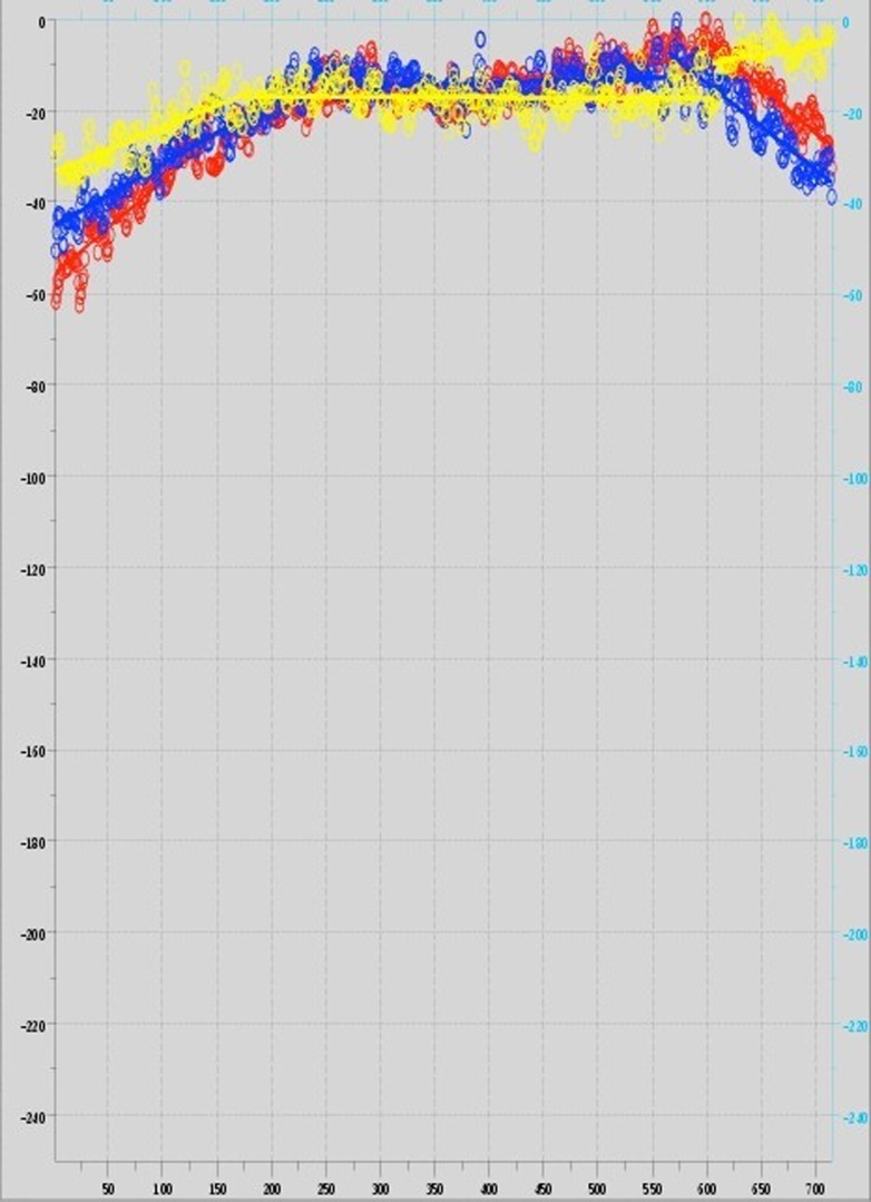
The “ideal” response from a well-aligned microscope with even field illumination is a consistently bright intensity with some allowable variance of illumination across the field of view. In practice, the intensity data from the international study often displayed regions in which the illumination was steadily increasing or decreasing (Fig. 3), had sudden illumination discontinuities, or had high variance. This suggests that many LSCMs in place in laboratories across the globe are not properly aligned. This validates the need for this algorithm and QF determination. A linear segmentation technique⁸ was used to quantify these observed types of departures from ideal illumination and factor them into the QF. The resulting estimated segmentations delineate regions of approximately linearly change or constant illumination and discontinuities and provided a means to estimate the variance (see fitted segmentations in Fig. 3). The fast algorithm associated with this technique, to the best of our knowledge, is the best method for capturing the important departures from ideal illumination observed in the data. The resulting slope and variance estimates were used in the development of the QF and were directed at penalizing nonlinearity and high variance.

Figure 3.

Plotted intensity data and the line segments [upper left to lower right (red); upper right to lower left (blue); and a center horizontal line (yellow)] for Microscope D. This scope exhibited increased illumination on the left, more stable central illumination, and decreasing illumination on the right. Also on the right, the yellow scan displays an apparent discontinuity. Each scan has been approximated by 3 optimally determined line segments whose slopes are used in the scoring function.

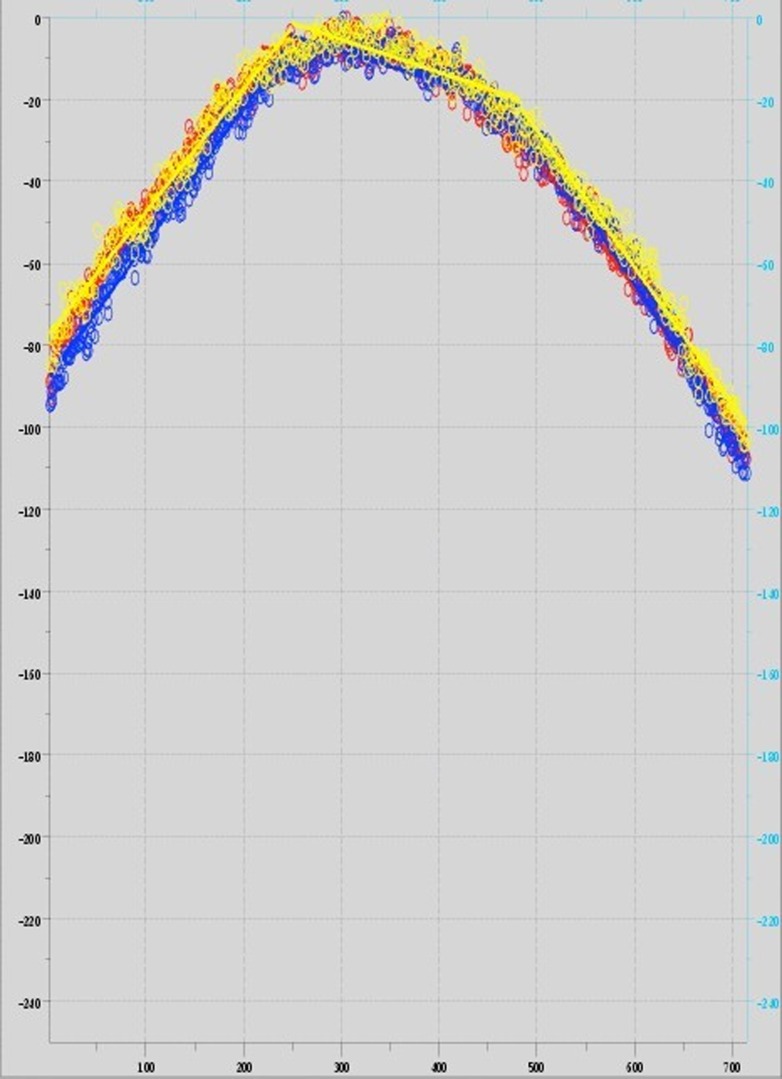
The scoring function was developed in 3 steps. In the first step, illumination responses were modeled by segmenting each intensity profile (2 diagonal and 1 horizontal) into 3 linear functions.⁸ This method captured consistent illumination in each scan by estimating 3 lines with similar intercepts and near-0 slopes. Quasiparabolic illumination responses (Fig. 4) generally yielded an initial line with positive slope, a terminal line with negative slope, and an intermediate line with near-0 slope. A perfect field illumination would yield 3 flat lines with 0 slopes.

Figure 4.

Plotted intensity data and the line segments [upper left to lower right (red); upper right to lower left (blue); and a center horizontal line (yellow)] for Microscope AM (see Supplemental Data for more information on this scope), exhibiting a quasiparabolic illumination profile and demonstrating the fit of the 3 line-segment approximations.

In the second step, root mean squared intensity (RMSI) and the length-adjusted absolute values of each of the 3 slopes were totaled across measurements, resulting in 4 variables for each microscope tested. These variables were augmented by 2 more: total absolute first differences (AFDs) and total absolute second differences (ASDs; Table 2). The non-RMSI variables were then log transformed to make their distributions more Gaussian.

TABLE 2.

Score Function Parameter Estimates

Term	Estimate	T statistic	P	Definition
Mean	−13.058	−0.601	0.28	Value when other variables are 0
RMSI	0.708	3.278	0.00082
LinMid	4.638	4.348	0.00002
LinRght	5.174	4.233	0.00003
FirstDif	−57.831	−1.308	0.096
ScndDif	44.981	1.091	0.14
RMSI2	−0.001	−2.665	0.0048	RMSI squared

I_s (i), Scaled illumination (Eq. 1 in Supplemental Data) at position i of scan s; η_s, number of non-0 scan s values; β_s (L), slope of scan s in line segment L: left = 1, middle = 2, or right = 3; η_s (L), its length. RMSI penalizes departures from the maximal intensity. Linear middle (LinMid) and linear right (LinRght) variables penalize illumination changes depending on their lengths. First differences (FirstDif) and second differences (ScndDif) penalize changes in adjacent and triplet positions. With the exception of RMSI, all variables are logged before computing the score function, defined as the sum of the product of the estimates and variables.

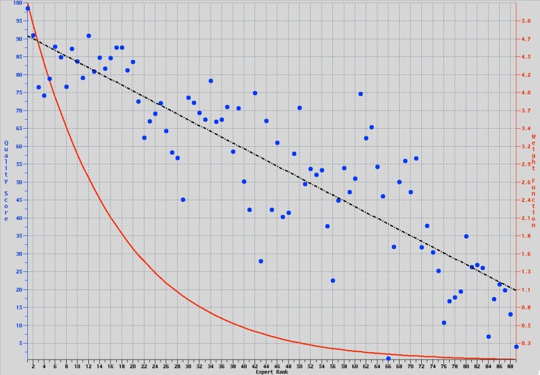
Multiple experts (n = 5) ordered the microscopes in an iterative method to refine the algorithm. The mean intensity, the aforementioned 6 variables, and their squares were subject to robust backward-model selection in regressions against the expertly ranked training set order.⁹ All square terms, except RMSI, dropped out, as did the scan's initial slope, presumably as symmetry typically rendered it redundant with the terminal line's slope. Investigation of each microscope’s influence on the resulting scoring function found 4 microscopes to be extremely influential. They were removed from the training set to ensure that they were not unduly controlling the parameter estimates. Although they were nonsignificant, elimination of AFD and ASD was found to lead to misordering of the top-ranked microscopes. It was asserted that this might be mediated by error-prone expert rankings of the bottom-ranked microscopes, as a result of the difficulty of determining relative rankings for microscopes showing poor performance. To account for decreasing ranking accuracy at high ranks, a weighting function was introduced to down weight the bottom-ranked microscopes and improve the scoring function on the top-ranked microscopes (Eq. 2 in Supplemental Data). This modification proved successful in generating a scoring function, acceptably ranking all of the microscopes in the training set (Table 1 and Fig. 4)

When the resulting algorithm was applied to the reserved 33 confirmatory microscopes, the resulting rankings were in agreement with the expert rankings (Fig. 5).

Figure 5.

Agreement between expert rankings and quality-score percentages (blue circles), showing the relationship is linear (dashed black line). The quality-score percentages were transformed from regression estimates of a score function, in which agreement with expert rankings was achieved only after down-weighting high-ranked scopes (red line; Eq. 2 in Supplemental Data).

The QF

The third step was to turn the scoring function into a more familiar quality-rating score or QF. The range of scores observed in all training microscopes that we examined was from 25 to 92. The score function was transformed to a percentage scale based on the 89 microscopes in the training set: quality score percentage = 100 × min (1, 1 min(1(scoring function − 24)/71)), which yielded values in our training data in a slightly smaller range than 0–100%, where a QF score of 100% indicated the highest quality. The minima introduced in the formula were needed to keep the values in range. MATLAB code, which scaled and segmented the triplicate measurements (input as a 3 column comma separated variable file), generated 6 regression variables, computed the score function, and out put the final QF as a percentage (the code is provided as Supplemental Data).

RESULTS

A scoring function was developed to produce a QF score, which measures the evenness of field illumination for WF microscopes and LSCMs. To accomplish this, a training set of illumination data from 89 microscopes was ranked independently by multiple light microscopy experts and used to build the algorithm. This proved to be successful in producing a robust and useful formula. The iterative process of ranking and refining the algorithm added accuracy and robustness to it, especially across multiple imaging modalities. The newly developed algorithm was then applied to illumination data from 33 “test” microscopes. Not only was the algorithm robust enough to rank LSCM data correctly, data similar to the data from which they were constructed also were able to properly rank WF microscopes, which were not used in developing or refining the algorithm. The validity of the algorithm is evidenced by the high degree of agreement between the final expert rankings and the QF percentages (see Fig. 5); an R² value of 74% was achieved. This is quite remarkable, given the expected variation between microscopes and the difference in image formation and detection between WF microscopes and LSCMs (see above sections).

Whereas the ideal QF score is 100%, this is not routinely achievable. Therefore, there a balance between ideal and achievable results was built into the scoring algorithm. A QF ≥ 83% was set as the minimum acceptable value (plots of all microscopes are in Supplemental Data), and this was based on no more than a 10% deviation in fluorescence intensity along the diagonal-intensity profile across the field of view and a 5% deviation across the horizontal-intensity profile data. These deviations were based on manufacturer’s specifications, as well as what had been established as routinely achievable.⁷ The QF percentages appear at the top of each microscope line intensity-profile plots in Supplemental Fig. 1. The QF percentages for the 33 independent confirmatory microscopes are shown at the top of each microscope image line intensity-profile plot scan in Supplemental Fig. 2. The shocking and concerning outcome was that most of the training scopes 77–89 failed to meet the QF scope of 83%. The test set was better with 14 of 33 passing the minimum QF score. These data were collected voluntarily and sent in as part of another project (uniformity of illumination), and therefore, one would have expected a higher number of passing scopes. These low QF scores support the need for testing scopes and for a metric to quantify the evenness of illumination, such as the QF score that we present here.

Malalignment of the illumination source, whatever type it was, may not have been readily apparent, or all systems would have been aligned all the time. For WF microscopes, alignment of the illumination source is typically done by the operator or core facility personnel. Once a misalignment is determined, realignment can be accomplished easily (see Fig. 1 for an example of a coupler that is simple to align). For example, microscope 31 had a QF score of 9.2 before alignment and a QF score of 88.4 after alignment (see test set.pdf in Supplemental Data). The dramatic improvement in the QF score was simply a result of the correction of the alignment and was accomplished easily once the need for realignment was determined. This points out the need for monitoring the illumination, as well as having a metric that alerts users and/or core facility personnel when alignment is necessary. The algorithm presented here can serve as that metric.

Low signal to noise, usually associated with LSCMs, can mask the actual state of alignment, both for aligned and misaligned microscopes. Thus, it is particularly important to check for even illumination, quantify it, and realign the system if need be. The graphs from the algorithm provide a visual representation of QF score, which then allows for more efficient corrective action to be taken. In some instances, this is as simple as improving the signal to noise of the image collection. In other cases, a service engineer will need to align the coupling between the laser light sources and the LSCM head.

DISCUSSION

The importance of an even illumination across the microscope field of view cannot be overstressed, even for nonquantitative imaging. Whereas the need for homogenous illumination might be obvious where intensity measurements are made directly, it is equally important when postacquisition techniques are applied, for example, colocalization, deconvolution, ratio imaging, morphology measurements, etc. One of the basic assumptions for all of these techniques is homogenous illumination. Even when no measurement or postacquisition techniques are used, nonhomogenous illumination distorts and even corrupts the image and potentially, the conclusions drawn from it.

The triplet intensity-scan procedure (2 diagonal + 1 horizontal-intensity line profiles) of a flat-field image presented here is fast and only requires simple specimens with uniform intensity. For fluorescence imaging, the test specimen could be a doped microscope slide,⁷ thin layer of fluorescent dye,^1,6 or Schott GG-475 glass.⁹ For brightfield imaging, no specimen is needed for field-uniformity testing. The algorithm and QF score calculation should be easy to incorporate into standard operating procedures, having minimal impact on overall microscope operation and far-reaching benefits. These benefits include a single test for multiple microscope modalities, the ability to track the illumination system, microscope alignment and light-source stability over time, and the generation of a single QF metric that is comparable across multiple imaging modalities.

The underlying contribution of the statistical development is to provide estimates that give an empirically derived relative weighting to nonlinearity (LinMid, LinRght) and illumination inhomogeneity (RMSI, FirstDif, ScndDif). In as much as there seems to be no theory to gauge their relative importance, the expert rankings and subsequent model selection serve as unbiased substitutes. Microscope failures of the test, i.e., a QF below 83%, were sometimes a result of high variance, as test images were collected with a low signal to noise. Simply recollecting the images with higher signal to noise could potentially raise the QF significantly; this is especially true for LSCM.

Whereas we have only demonstrated optical microscopy in this paper, this technique and algorithm would be applicable to any imaging modality where there is a directed illumination source, including, but not limited to, plate readers, slide scanners, electron microscopes, and gel boxes.

Future Directions

As the number and diversity of imaging platforms that use this algorithm increase, so will the precision of the outcome QF score. Therefore, we encourage users to submit their data to us (contact richard.cole@health.ny.gov for submission instructions). This will thereby provide information for the future improvement of the output QF score for all researchers by use of the algorithm. To achieve full use of this algorithm, we are planning on converting the MATLAB code over to a readily accessible Fiji plug-in.

REFERENCES

- 1.Model MA, Blank JL. Concentrated dyes as a source of two-dimensional fluorescent field for characterization of a confocal microscope. J Microsc 2008;229:12–16. [DOI] [PubMed] [Google Scholar]
- 2.Kedziora KM, Prehn JH, Dobrucki J, Bernas T. Method of calibration of a fluorescence microscope for quantitative studies. J Microsc 2011;244:101–111. [DOI] [PubMed] [Google Scholar]
- 3.Zucker RM, Price OT. Practical confocal microscopy and the evaluation of system performance. Methods 1999;18:447–458. [DOI] [PubMed] [Google Scholar]
- 4.Matthews C, Cordelières FP. MetroloJ: an ImageJ plugin to help monitor microscopes' health. Image J User & Developer Conference. Mondorf-les-Bains, Luxembourg,2010. [Google Scholar]
- 5.DeRose PC, Resch-Genger U. Recommendations for fluorescence instrument qualification: the new ASTM Standard Guide. Anal Chem 2010;82:2129–2133. [DOI] [PubMed] [Google Scholar]
- 6.Murray JM, Appleton PL, Swedlow JR, Waters JC. Evaluating performance in three-dimensional fluorescence microscopy. J Microsc 2007;228:390–405. [DOI] [PMC free article] [PubMed] [Google Scholar]
- 7.Stack RF, Bayles CJ, Girard AM, Martin K, Opansky C, Schulz K, Cole RW. Quality assurance testing for modern optical imaging systems. Microsc Microanal 2011;17:598–606. [DOI] [PubMed] [Google Scholar]
- 8.Killick R, Fearnhead P, Eckley IA. Optimal detection of changepoints with a linear computational Cost. J Am Stat Assoc 2012;107:1590–1598. [Google Scholar]
- 9.Paulson AS and Delehanty TA. In Computer Science and Statistics: Proceedings of the 14th Symposium on the Interface (Heiner KW, Sacher RS, Wilkinson JW, eds), Springer Verlag, New York, 1983;52–57. [Google Scholar]
Associated Data
This section collects any data citations, data availability statements, or supplementary materials included in this article.