Any Way You Slice It—A Comparison of Confocal Microscopy Techniques

Abstract

The confocal fluorescence microscope has become a popular tool for life sciences researchers, primarily because of its ability to remove blur from outside of the focal plane of the image. Several different kinds of confocal microscopes have been developed, each with advantages and disadvantages. This article will cover the grid confocal, classic confocal laser-scanning microscope (CLSM), the resonant scanning-CLSM, and the spinning-disk confocal microscope. The way each microscope technique works, the best applications the technique is suited for, the limitations of the technique, and new developments for each technology will be presented. Researchers who have access to a range of different confocal microscopes (e.g., through a local core facility) should find this paper helpful for choosing the best confocal technology for specific imaging applications. Others with funding to purchase an instrument should find the article helpful in deciding which technology is ideal for their area of research.

INTRODUCTION

Wide-field fluorescence microscopes achieve excellent resolution, contrast, sensitivity, and acquisition speeds. However, for thicker specimens, the out-of-focus features add a blurry haze to each image plane, reducing contrast. Many 3-dimensional (3D) imaging technologies have been developed to remove this out-of-focus haze and improve contrast, and thereby resolution, in the fluorescence microscope. The confocal laser-scanning microscope (CLSM) was first conceptualized and patented in 1957 by Marvin Minsky.¹ However, it was the implementation and commercialization of the CLSM in the late 1980s—specifically for fluorescent biologic samples— that really moved the CLSM to the mainstream of biologic research.² The development of a robust and reliable instrument, the use of rapidly scanning mirrors instead of slowly moving the sample, and the ability to remove out-of-focus blur to produce a series of thin optical slices of the specimen in 3D revolutionized fluorescence imaging. Images of a single image plane in the middle of a very thin sample (<5 μm), a sample of intermediate thickness (∼20 μm), and a thick sample (∼50 μm), imaged in wide-field or CLSM modes, demonstrate the need for confocality for thick samples (Fig. 1). For thin samples, there is only a slight advantage using confocal imaging (compare Fig. 1a and b), but for thicker samples, the removal of out-of-focus blur from each image section is crucial for visualizing and measuring features of interest in the specimen (compare Fig. 1c and d and 1e and f).

Figure 1.

Comparison of 3D imaging techniques. Comparison of wide-field (a, c, and e) and CLSM (b, d, and f) images of samples of various thicknesses. A thin sample of cultured epithelial cells labeled with DAPI, Alexa 488-phalloidin (actin filament strain), and MitoTracker Red mitochondrial stain does not show a huge difference between wide-field (a) and CLSM (b) images. Intermediate thickness sample images of an ∼20-μm-thick mouse kidney section, labeled with DAPI, Alexa 488-wheat germ agglutinin (membrane stain), and Alexa 568-phalloidin (actin filament staining), show significant improvement of image quality and specimen detail in CLSM (d) vs. wide-field (c) images. Thick sample images of a 3D culture of MCF-10A mammary epithelial cell spheroid of ∼50 μm thick, labeled with a nuclear green fluorescent protein fusion and a red fluorescent protein fusion marking the membranes, again show significant improvement in CLSM (f) vs. wide-field (e) images. Scale bars, 20 μm.

The CLSM has continued to evolve over the decades. It is now commonplace in essentially all biomedical research institutions. It is the foundation of newer technologies such as multiphoton microscopy³ and many superresolution techniques.⁴ The CLSM is inherently slow because a digital image is built up point by point as a small focused laser beam is scanned across the specimen. However, the widespread use of the confocal microscope for imaging of living specimens^5–15 and the need to image rapid biologic processes have led to the development of new confocal modalities for rapid imaging. The concept of using a spinning disk to generate an image is very old and was first proposed by Nipkow in 1884.¹⁶ In fact, this process was used to break up video frames into discrete units for transmission, enabling the development of the first television images in the 1920s. The key to image formation with the spinning disk is that holes in the disk are positioned in a spiral array so that when the disk is spun and data are collected over time, the entire image area can be viewed. In turn, an array-based detector or camera is needed to generate an image. This same principle was used to develop the first potentially commercial spinning-disk confocal instrument in 1968.¹⁷ However, commercial spinning-disk confocal microscope (SDCM) platforms were not prevalent until around the same time as the CLSM in the late 1980s. Early versions of the SDCM suffered from the drawbacks that light sources were not very bright, and camera-based detectors were not very sensitive, so the SDCM had limited application for biologic samples at that time. It was the invention that reinvigorated the commercial SDCM market by the Yokogawa Electrical Corporation (Tokyo, Japan) in 1992. They invented a microlens array disk perfectly coupled to the pinhole array disk to focus the light into the pinholes (U.S. patent number 5,162,941). Interestingly, with the advent of high-powered diode lasers, the original single-disk design (lacking the microlens array disk) is currently making a comeback. Another area of development in rapid 3D imaging is the resonant scanning CLSM (RS-CLSM). This development has been made possible by fast resonant frequency-scanning galvanometer mirrors, creative mechanisms to correct for image distortions introduced by the variable pixel dwell times as the mirror scans the laser beam back and forth, and more-sensitive detectors. These resonant-scanning confocal systems have much the same properties of the more traditional CLSM, with the added benefit of the ability to scan rapidly and image faster biologic processes.¹⁸ Finally, affordable grid confocal systems have been developed for wide-field microscopes^19,20 without the need for scanners and laser-based excitation. These systems depend on a grid pattern being superimposed onto the image plane and the collection of multiple images to separate in-focus and out-of-focus light.

This article will present 4 modes of confocal imaging: the grid confocal, the CLSM, the RS-CLSM, and the SDCM. An overview of how each technique works, its strengths, ideal applications, its weaknesses, and recent developments will be presented for each technology. Another popular, sensitive, and useful 3D imaging technique is wide-field deconvolution. This technique is ideal for thinner samples (<30 μm), is reviewed in several articles,^10,21–29 and will not be discussed here. The intent is that this article will assist researchers in understanding which technology is ideal for their given application or best for an equipment purchase for their laboratory or core facility.

GRID CONFOCAL MICROSCOPE

How It Works

The grid confocal microscope was designed by Neil et al.²⁰ and Wilson³⁰ as an add-on to the wide-field microscope and was subsequently commercialized [e.g., ApoTome by Carl Zeiss Gesellschaft mit beschränkter Haftung (Jena, Germany), OptiGrid by Qioptiq (Munich, Germany)]. This technique is often referred to as structured illumination microscopy (SIM); however, the term “grid confocal” will be used here to avoid confusion between this basic technology and the more complex super-resolution SIM technique developed by Gustafsson.³¹ The grid confocal relies on the placement of a movable grid pattern in the excitation light path between the light source and the sample, which projects a grid pattern into the image plane. Three snapshots of the fluorescent sample are recorded with the grid of horizontal lines in 3 different positions. A simple image calculation (essentially subtracting each image from the other 2 and summing the squares of these differences) removes the out-of-focus light, leaving behind a single image containing only the in-focus information. A “regular” wide-field image can also be computed by simply summing the 3 images together. The grid confocal technique applied to a 20-μm-thick kidney section demonstrates the ability of this technique to perform optical sectioning for specimens of intermediate thickness (compare Fig. 2a and b).

Figure 2.

Performance of the grid confocal microscope. Comparison of wide-field (a) and grid confocal (b) images for the same kidney sample as shown in Fig. 1c, d. The grid pattern is readily apparent when projected into a thin specimen (c) but is lost in the haze for an ∼50-μm-thick specimen (d). The CLSM (e) gives a much higher S/N, more accurate, and artifact-free image of the sample than the grid confocal (f). Scale bars, 20 μm.

Best Applications

Grid confocal, sometimes dubbed “the poor man’s confocal,” is an affordable add-on to an existing fluorescence microscope. It functions with standard wide-field illumination sources and does not require the purchase of an expensive laser combiner and lasers. The price is within the realm of a single research laboratory budget and can provide for routine 3D imaging in the laboratory on relatively thin specimens (∼20 μm). The quantitative nature of the fluorescence image data has been established, making this a useful tool for 3D fluorescence imaging.³²

Limitations

There are several drawbacks of the grid confocal technique. First, for thicker specimens, the grid pattern is lost in the haze, and the technique fails. Raw images show that the projected grid pattern (taken before the calculation for optical sectioning is applied) is clearly visible on a thin specimen (∼5 μm thick; Fig. 2c). On the other hand, the grid pattern for a thick sample (∼45 μm) is obscured by the haze of out-of-focus light blur (Fig. 2d). The resulting grid “confocal” image (Fig. 2f) is plagued by noise and lack of contrast, even though this same specimen was easily imaged by a CLSM (Fig. 1d). Because the grid pattern must be preserved throughout the specimen, the grid confocal technique is usually limited to specimens that are at most 20 μm thick.

A second limitation of the grid confocal is that it is prone to artifacts. This can be a hindrance for both image presentation and image analysis. The grid pattern is often observed even after processing is complete. With careful alignment before each acquisition session, the grid can be made less obvious, but contrast enhancement often reveals an underlying residual grid pattern. Also, because the algorithm relies on the subtraction of images, it is highly sensitive to noise. Despite smoothing (which is built into the optical-sectioning algorithm), the grid confocal images may be noisy and have a “mottled,” unnatural appearance (Fig. 2f).

A third limitation of grid confocal is its relatively slow speed. Three images (with the grid pattern shifted to a different position in each image) must be acquired for each focal plane and for each color channel, making the temporal resolution at least 3 times slower than standard wide-field imaging. Additionally, a small amount of time is also required for image processing to generate the final 3D image without out-of-focus blur. Finally, because the grid confocal relies on 3 sequential images to generate a single confocal slice, the technique is not appropriate for fast dynamic live-cell imaging where the sample can move in the time between each of the 3 image frames. However, newer implementations use piezo motors to rapidly shift the grid pattern and, when combined with fast cameras [Scientific CMOS (sCMOS), Andor, Belfast, Northern Ireland, Hamamatsu (Tokyo, Japan) or PCO AG (Kelheim, Germany)], can measure slower live-cell dynamics. Taken together, these limitations mean that the use of a CLSM or an SDCM is highly preferred if one is available.

New Developments

Because a different grid size is required for different objective magnifications, early implementations of the grid confocal required changing the grid and recalibrating the device for each objective lens. More recent versions of the grid confocal have a set of grids mounted on a motorized drive, so that the calibration for all objectives can be performed together. In addition, with faster 64-bit computers, the processing time to calculate the optical sections has become almost negligible. As mentioned above, the use of piezo motors has improved the grid confocal speed. The introduction of new sCMOS cameras promises to deliver larger fields of view. Thus, speed of capture for the grid confocal can be increased by taking fewer images of larger specimen areas.

CLSM

How It Works

The optical principle of a CLSM is quite simple, yet elegant. Light from a laser beam is focused down to a small spot in the specimen, exciting fluorescence in the entire cone of illumination (Fig. 3A). Fluorescence emission from the in-focus plane is imaged through a pinhole onto a detector, which measures the fluorescence intensity for this one spot (which becomes 1 pixel of the image). Fluorescence from out-of-focus planes is blocked by the pinhole, which is said to be confocal with the focal point of the objective lens (Fig. 3B). The focused spot is scanned back and forth across the specimen to generate an image pixel by pixel. To form a 3D data set, the focus can then be changed and another image generated at the new focal depth. Successive images are collected at various focus depths to generate a 3D image stack.

Figure 3.

Schematic diagram of the CLSM. The excitation laser beam light path (A) and emission light path (B). The solid blue lines in (A) represent the excitation laser that is focused onto the specimen. The solid green lines in (B) show that emission light from the focal plane passes through the pinhole aperture and is detected by the PMT. However, the dashed gray lines show that out-of-focus light will be blocked, will not pass through the pinhole, and will not be detected by the PMT. Reprinted with permission from Methods in Cell Biology V123, p113-134, 2014.

The CLSM is a rather sophisticated arrangement of optical, mechanical, and electronic components, with advanced software orchestrating the image acquisition (Fig. 4). To start with, the CLSM illuminates the specimen with lasers of various wavelengths (available from UV to infrared). Lasers are required because they produce an intense beam that can be readily focused down to a tiny spot that is required for the CLSM. The confocal scan head is then attached to one of the microscope’s camera ports. Strategically placed galvanometer mirrors within the scan head guide the laser beam through the objective lens and back and forth and up and down across the specimen. One high-speed galvanometer mirror rapidly scans the laser beam horizontally along the x axis. A second high-speed galvanometer mirror advances the laser beam more slowly line by line along the vertical y axis (Fig. 4). For high-resolution imaging, the fluorescence intensity is typically collected while the laser beam is scanning from left to right. Modern confocal microscopes use acousto-optic tunable filters (AOTFs) to rapidly turn lasers on and off, attenuate laser light, and to select which color of laser light is exciting the sample. The AOTF control is very fast because it uses rapid electronic signals. For example, it is used to turn off the laser beam during the millisecond backward scan time as the mirrors are reset to the start of the scan line at the leftmost side of the digital image. The y axis mirror is then adjusted to scan the next line in the image. High numerical aperture (NA) objective lenses are engineered to achieve high resolution and high light throughput and to minimize optical aberrations. Instead of visualizing the specimen by eye or using a camera, the fluorescence from the sample is collected by the objective lens, rescanned by the galvanometric mirrors, and then focused through a confocal pinhole, onto a point detector or photomultiplier tube (PMT) (Figs. 3 and 4). The PMT has a light-sensitive photocathode that converts photons of light that hit the detector into photoelectrons that are then amplified by a series of dynodes. The analog PMT signal is then digitized to a gray level (usually 12 bit, so a value between 0 and 4095) and stored by a computer along with the precise x, y location of the focal point. PMTs are not very sensitive; they only have a quantum efficiency (QE) of ∼20% (i.e., 20% of the photons that hit the photosensitive photocathode are detected). However, they are very good amplifiers because each photon signal that is detected is amplified thousands of times. As the laser is scanned across the sample, the PMT measures the light intensity across the sample. PMTs can detect a 25- to 50-photon signal in as little as 1 μs, thus capturing a 1 megapixel (1024 × 1024) image in ∼1 s. Laser power, filter choice, focus control, galvanometer mirror speed, pinhole size, PMT voltage, and nearly every other parameter of the confocal are all computer controlled. As the PMT detects the fluorescence pixel by pixel across the sample, the computer builds up an image of the specimen on the computer screen. For multicolor imaging, secondary and sometimes tertiary dichroic mirrors are used to split emission light of different colors onto different PMT detectors (Fig. 4). Most CLSMs have multiple discrete PMT detectors for simultaneous acquisition of 2–5 fluorescent probes (can image up to 5 dyes with no postprocessing) or else have an integrated array of as many as 32 PMT elements (can image up to 10 dyes; requires postprocessing/spectral unmixing).

Figure 4.

Basic CLSM light path. Schematic diagram of the CLSM light path with blue excitation light selected by the AOTF. The light is focused onto the sample by the objective lens and then scanned across the sample by the x and y galvanometer mirrors. Emission light is focused by the objective lens, descanned by the mirrors, and reflected toward the detection light path by the primary dichroic mirror. In-focus light is selected by the pinhole aperture. The secondary dichroic mirror splits the green emission light and directs it to be detected by PMT1, and the red emission light passes and is detected by PMT2.

The x and y pixel size of the CLSM, determined by how far the mirrors move the focused laser beam between pixel intensity readings, provides flexibility for zooming and panning around the microscope’s field of view (FOV). In principle, the minimum pixel size is only limited by how precisely the mirrors can move the laser beam. In practice, the optical resolution is much lower than this so that over sampling—imaging with pixels that are too small—should be avoided.³³ Optimal optical resolution and sampling can be calculated based on the NA of the objective lens and the wavelength of emission light, or they can be measured using subresolution fluorescent microspheres.³⁴ The axial resolution is determined by the focal depth of the objective lens (typically as NA is increased, focal depth is decreased), the size of the confocal pinhole, and the distance between successive images in 3D. The variable pinhole on the CLSM makes it ideal for maximal resolution with many objective lenses of different magnification and NA. It is typically set to 1 airy unit (AU) optimizing z axis resolution and collecting ∼80% of the light from the pixel location. However, slight increases in the pixel size up to even 2 AU have a minimal effect on z axis resolution while improving sensitivity by letting more light through the pinhole. The z axis spacing between images should be set at about one-third the axial resolution.³⁴ Other important aspects of the CLSM are the scan speed and scan averaging. Slower scan speeds will result in better signal to noise (S/N) because each pixel intensity will be integrated longer building signal and reducing noise. However, photobleaching of the fluorophore will also increase. A good compromise is to average multiple images or each image line multiple times to minimize photobleaching (i.e., shorter pixel dwell times) while increasing S/N. Other publications provide more detail on ideal settings for quantitative confocal image collection and analysis.^35–38

Best Applications

The CLSM is the most versatile 3D imaging system and is the best choice for a wide range of both routine and advanced imaging applications. Using galvanometers to scan the laser beams across the specimen gives the CLSM unparalleled flexibility to match the FOV with the resolution and the specimen of interest. For example, a single z axis image of the entire FOV of a specimen can be scanned at low zoom with 512 × 512 pixels in ∼1 s to visualize many cells (Fig. 5a). Subsequently, using a higher zoom setting, the nucleus of single cells can be individually selected for high-resolution imaging (Fig. 5b). A high-resolution through-focus series (or “z-stack”) of ∼20 image planes is scanned with the optimal pixel size of ∼0.1 μm in ∼10 s (Fig. 5b). Returning to the low-zoom overview image and selecting the next nucleus for high-resolution 3D image acquisition take only a few seconds. This overview-and-zoom method avoids high-resolution sampling of empty areas in the FOV and can make the CLSM nearly as fast as the SDCM while maintaining the best resolution optical microscopy can offer. For tissue imaging, high NA objective lenses with low magnification (e.g., 20×/0.75 NA air or 40×/1.4 NA oil immersion) can be used to capture large fields of view with little or no compromise in resolution.

Figure 5.

Demonstration of the flexibility of the CLSM for scanning different sizes of the FOV with optimal resolution. Fixed HeLa cells labeled with DAPI (blue) and Alexa 488-H2AX (green), captured as a low-resolution overview image by scanning the entire FOV of a 63×/1.4 NA oil objective lens on a CLSM (a). A maximum-intensity projection of a 10-image z-stack of a zoomed-in area of the same sample as in (a) with an optimal pixel size of 0.1 μm (b). Maximum-intensity projection of a z-stack of a fixed rat brain section, imaged with a 20×/0.8 NA objective lens on a CLSM showing the complete SCN structure (c) labeled with DAPI (blue), arginine-vasopressin (green), and the proto-oncogene, C-Fos (red). Zoomed-in image of (c) showing that individual nuclei can be easily quantified for number and intensity from this large FOV high-resolution CLSM image (d). Scale bars, 10 μm (a and b) and 100 μm (c and d).

In turn, the CLSM can be used for moderate resolution applications such as to count nuclei or identify positive cell populations when subcellular resolution is not required. Large sample areas (e.g., ∼500 × 500 μm) can be imaged at lower magnification with high resolution using a 20×/0.80 NA objective lens and 2048 × 2048 image pixels with a resolution of 0.25 μm (Fig. 5c). The CLSM can capture a large FOV for a complete specimen of interest [e.g., the entire suprachiasmatic nucleus (SCN) structure (highlighted in yellow in Fig. 5c)] at high enough resolution to image each individual nucleus and identify positive nuclear staining within an entire 20-μm-thick rat brain section].

The CLSM is the most versatile confocal in a number of other respects as well. As described above (Fig. 3), the CLSM uses a pinhole to achieve optical sectioning: a smaller pinhole produces a thinner optical slice, but a larger pinhole lets more light through to the detector. In the CLSM, the pinhole size can be adjusted to match the resolution of the objective lens and the color of light. In addition, the pinhole can be made larger to image light-sensitive specimens such as living cells, or the pinhole can be closed down to a smaller size for bright, stable samples when maximal resolution and 3D-sectioning ability are required. For multicolor imaging, the CLSM can have up to 5 detectors working simultaneously or 2–3 detectors collecting different colors sequentially. In either case, 5-color imaging can be achieved routinely in a reasonably straightforward manner. With spectral array detectors (see advances below), even >5 colors can be imaged routinely. Because the galvanometer mirrors can direct the laser beam to make any type of pattern anywhere in the sample, the CLSM is also an excellent platform for probing living cells with photoactivation, photoconversion, or photobleaching (e.g., fluorescence recovery after photobleaching).^39,40

In general, the CLSM is slow because it samples each pixel in the image sequentially. On the other hand, the instrument can be optimized for speed for specific applications by compromising resolution and/or spatial information. For instance, small cells like neutrophils can be imaged using a small region of interest (ROI). Spatial resolution can be sacrificed for speed using larger spacing for the y axis scanning and less averaging. Images will not be optimal for visualization, but the fluorescence intensity information is still quantitative. These types of parameters were used to image endosome-mitochondrial interactions occurring in just seconds in live neutrophils.⁴¹ In addition, spatial information can be sacrificed for speed by using the line-scanning feature. A time versus distance kymograph image can be generated with temporal resolution on the milliseconds’ timescale. This technique can be used for many applications including calcium imaging⁴² and imaging of focal adhesion dynamics.⁴³

Limitations

The main weaknesses of the CLSM are speed and sensitivity. It takes ∼1 s per image to collect a 1024 × 1024 pixel image with a 1 μs pixel dwell time. This sounds pretty fast, but for 4 sequential fluorophore channels, averaging of 4 scans for each image (to improve the S/N), and 20 images in a z-stack to capture the entire volume, each 3D data set (such as the one shown in Fig. 5b, d) can take several minutes. Newer RS-CLSMs overcome some of these speed issues by using rapid scanning mirrors (see below). For live-cell imaging, the CLSM causes a lot of phototoxicity because it relies on a highly temporally and spatially localized laser spot. Phototoxicity can be minimized by using lower laser powers, higher scan speeds, and line averaging. The lower-sensitivity PMT detectors compound this problem, but newer detectors are overcoming this issue (see below). Despite these weaknesses, the CLSM is probably the best general-purpose confocal and a workhorse of most life sciences research labs, especially for thick-fixed specimens.

New Developments

Acousto-optic (AO) devices have enabled the speed revolution for the CLSM.⁴⁴ These devices typically function through the application of acoustic waves across a birefringent crystal, changing the crystal’s refractive index. Variable frequencies of AO waves cause refraction and bending of different wavelengths of light, giving rise to highly tunable wavelength-specific bending. Thus, different wavelengths of light can be bent into or out of the light path of the microscope. Devices of this type include acousto-optic deflectors that can be used for laser beam scanning, acousto-optic modulators for attenuating laser light, AOTFs for laser beam selection and attenuation, and acousto-optic beam splitters (AOBSs). AOBS devices are essentially AOTFs that are used as a substitute for dichroic mirrors to spectrally combine or separate laser light. This high-speed modulation (in microseconds) allows for 1) rapid multicolor imaging without crosstalk between signals; 2) high-precision laser attenuation for localized photobleaching and/or photoactivation of fluorescent molecules; and 3) the ability to attenuate laser excitation during the “back-scan” and when scanning outside of the image area, minimizing sample photobleaching and phototoxicity.

Gallium arsenide phosphide (GaAsP) PMTs offer one way to improve the sensitivity of PMTs by using a more-sensitive photocathode material: GaAsP. They are efficient in the 400–650 nm range with a QE of ∼40% and an amplification of ∼1500 times.⁴⁵ They are not highly sensitive outside of this wavelength range, so they are typically used in combination with traditional PMTs in order to efficiently detect light from the UV to the infrared.

Hybrid detectors (HyDs) take advantage of the high dynamic range of the PMT technology and the high sensitivity of the avalanche photodiode (APD) technology. A GaAsP PMT photocathode is used for the initial photon detection. These electrons then impact an APD sensor, and the signal is further amplified by ∼100-fold. The overall result is an ∼150,000-fold amplification in signal.

Array-based spectral detectors provide the ability to image the entire fluorescence emission spectrum from a sample with multiple fluorescent dyes with 1 or 2 image scans. With adequate reference spectra for each of the dyes/fluorophores, as well as sample autofluorescence, 8–10 signals can be imaged simultaneously. The signal is then separated by postprocessing using reference spectra and spectral unmixing algorithms. These systems come with an increased price tag, and they require careful calibration and quality control metrics⁴⁶ but allow for high-speed multicolor imaging.

Semiconductor-based diode lasers are currently the most common laser light source for CLSMs. They are compact, offer a stable high-quality beam, and can be directly modulated at high frequencies without the need for AO devices. They have long lifetimes in the range of 10,000–50,000 h and do not generate a significant amount of heat. Their small size has resulted in more compact CLSM systems.

White light lasers consist of a low energy-pulsed infrared fiber laser (80 MHz) that is amplified by a diode-pumped laser amplifier. The light that is generated covers the visible spectrum from 470 to 670 nm, and an AO device is used to select light bands that are 1–3 nm in width. The white light laser has a significant cost associated with it, but in principle, it could be the only laser on a CLSM. Thus, the cost could be offset because there will not be a need to purchase many individual single-wavelength diode lasers. The main downside of the white laser is that each wavelength has only a few milliwatts of power; therefore, some photobleaching or photoactivation experiments are not possible. However, this is offset by the flexibility of having so many laser excitation wavelengths to choose from.

RS-CLSM

How It Works

RS-CLSM technologies achieve rapid scanning by using galvanometric mirrors that oscillate at a fixed frequency and undergo gradual acceleration and deceleration while scanning and imaging.¹⁸ The image is usually collected on both the forward and the back scan, so speed is drastically increased. The frequency for scanning a single image line is 4–16 kHz (compared to 1–3 kHz for traditional scanners), allowing for the acquisition of a 512 × 512 pixel image frame at upward of 30 frames per second. Because traditionally, the pixel clock is the same for each pixel location but with the RS-CLSM the pixel intensity information is collected while the mirrors are accelerating and decelerating, the raw image data are distorted. In addition, the pixel information on the backward scan is reversed and needs to be inverted in order to generate the image properly. Nonetheless, the speed of the scan mirrors is well known, and it can be used to calculate or measure the effective pixel dwell times across the image. Then, software can be used to compensate for the variable pixel dwell times and to reverse the back scan image data to the proper orientation to generate confocal images.

Advantages

The RS-CLSM has many of the advantages of the traditional CLSM. The FOV is variable, although not quite as flexible as the CLSM. The pinhole size can be varied for optimal high-resolution 3D imaging at different magnifications with objectives of variable NA. The instrument has the ability to photoactivate, photoconvert, or photobleach specific ROIs across the sample. In addition, the rapid speed makes imaging of fast biologic processes such as protein transport, lipid diffusion, and calcium fluctuations possible. The faster scanning of resonant scanners should lead to a reduced photobleaching and potentially reduced phototoxicity to living samples.⁴⁷

Limitations

The resonant-scanning galvanometers are not as flexible as the traditional galvanometers: they resonate at a particular fixed frequency, so the pixel dwell time is fixed by the chosen size of the FOV. In addition, because the pixel dwell time is well under 1 μs, for most specimens, there are very few photons collected in each pixel, resulting in a noisy image. Averaging (either frame by frame or line by line) dramatically improves the S/N in the image, but too much averaging lowers the scan speed, negating the speed advantage of the RS-CLSM. Fortunately, most commercially available RS-CLSMs are equipped with traditional galvanometers as well, giving the user the choice to scan very fast (with the resonant galvanometers) or very precisely (with the traditional galvanometers).

New Developments

The development of more-sensitive GaAsP PMTs and HyDs (see above) has been essential to allow high S/N imaging at the rapid speeds made possible by the RS-CLSM. Also, some resonant-scanning systems now allow for simultaneous operation of the 2 sets of galvanometers: the resonant galvanometers can scan the entire sample very rapidly, whereas the traditional galvanometers can direct a different laser to photobleach, photoactivate, or otherwise stimulate the specimen.

SDCM

How It Works

The SDCM works in a fundamentally different way than the traditional or the RS-CLSM. In the spinning-disk confocal, fluorescence is excited and imaged from multiple points across the sample simultaneously. Therefore, the SDCM uses an array-based detector (i.e., a camera) rather than a PMT point detector. For the Yokogawa-based SDCM, a laser light source is defocused to a larger laser beam spot (Fig. 6). That larger laser beam spot is then translated into ∼1000 small focused laser beam spots by the microlens array disk. These laser beam spots then pass through a dichroic mirror and are perfectly aligned to pass through corresponding pinholes on the pinhole array disk. The laser spots are then focused by the objective lens onto the sample. As the coupled microlens array disk and pinhole array disk are spun at 5000–10,000 rpm, the entire FOV will spend some time illuminated with a focused laser beam spot. It is essential that the rotation of the spinning disk and the camera exposure time are coupled so that all locations within the FOV receive an equal number of laser beam exposures during the camera exposure time. Otherwise, image artifacts such as line patterns in the images will be readily apparent. Emission light from the focal plane is then focused by the objective lens back through the pinhole array and reflected off of the dichroic mirror toward the camera (Fig. 6). Emission light arriving at the camera is then integrated for a fixed exposure time and digitized to generate an image. Automated motorized focusing is used to move the objective lens up and down in order to generate a 3D image stack. A secondary dichroic mirror can be used along with cameras to generate multiple images simultaneously (Fig. 6). For imaging of >2 colors, emission filter wheels or multicolor splitters can be introduced in front of the cameras but will result in reduced imaging speed and/or spatial resolution.

Figure 6.

Basic SDCM light path. Schematic diagram showing blue laser light passing through the microlens array disk and being focused through the dichroic mirror and through the pinhole array disk. These 2 disks along with the dichroic mirror spin as 1 unit. As the disk spins, many laser beam spots are focused onto the sample by the objective lens and are scanned across the sample in the FOV. Emission light from the sample is focused by the objective lens back through the pinhole array disk, is reflected off of the primary dichroic mirror, and split into green and red emission channels by the secondary dichroic mirror. In this example, 2 camera-based detectors are used to generate images of green and red stains.

Advantages

The SDCM is ideally suited for rapid 2-D or 3D imaging, particularly of relatively thin (∼40 μm or less) living samples.^7,48–50 Three successive frames of a sequence of images collected at a rate of 1 frame every 3 s (Fig. 7) show that the SDCM can capture the rapid dynamics of microtubule movements in living cells labeled with an enhanced green fluorescent protein-tubulin protein fusion (eGFP-tubulin). The fact that the laser light is split into many focused laser beam spots and that each location in the sample is exposed to lower-power excitation light for very short times with multiple passes of the spinning disk results in significantly reduced photobleaching and presumably phototoxicity compared with a CLSM.⁵⁰ Each point within the sample is exposed to a focused laser beam spot thousands of times per second for tens of microseconds each time. This signal is then integrated over the milliseconds’ exposure time of the camera. However, each exposure is to a much lower light density laser spot than that found in a single focused laser beam spot on a CLSM. In fact, on the CLSM, each spot within the sample is only exposed to light once for a few microseconds but at hundreds- to thousands-fold higher intensity. SDCMs are more sensitive with the high sensitivity of camera technologies of 70–95% QE when compared to 20–40% with PMTs. In addition, the hardware components of the SDCM are much less sophisticated than the CLSM and often lead to lower service contract expenses and/or repair costs and less instrument downtime. The SDCM is ideally suited for live-cell imaging, particularly when observing fast cellular dynamics.

Figure 7.

Live-cell SDCM time series images. Successive frames of a time-lapse sequence show that microtubule dynamics in smooth muscle cells can be observed by imaging eGFP-tubulin using a 60×/1.4 NA oil objective on a Yokogawa SDCM (a–c). A zoomed-in time overlay image shows isosurfaces of the microtubules and changes in microtubule location and length (d). The differences in microtubule length between successive frames are modeled as cyan showing the location of the microtubules in frame (a). The green isosurfaces represent changes in microtubule position and length between frame (a) and frame (b). The red isosurfaces represent changes in the microtubule position and length from frame b to c. Isosurfaces were calculated and generated using Imaris software from Bitplane Incorporated (Zurich, Switzerland). The yellow arrowhead denotes the same location in each frame. The timescales in a–c are shown in seconds. Scale bars, 10 μm.

Limitations

There are several major drawbacks of the SDCM that limit its versatility, making it less than ideal for many 3D imaging applications. First of all, currently, nearly all SDCMs rely on the highly sensitive electron-multiplying charge-coupled device (EM-CCD) camera technology for rapid imaging. The EM-CCD sensors have upward of 95% QE and amplify signals up to 1000-fold with the electron-multiplying gain. They are also more sensitive than traditional (interline) CCD cameras because of their large 16 × 16 μm pixels. The sensitivity, however, comes with a price: with such large pixels, there are only 512 × 512 pixels on the entire sensor. This results in a low-resolution image from a zoomed-in area of the center of the FOV. With a high-magnification 63×/1.4 NA lens, often the FOV is only the size of one single cell. The FOV is significantly smaller (Fig. 8, inner square) than the FOV on a CLSM (Fig. 8, outer square), so the SDCM cannot take full advantage of high-NA low-magnification objective lenses in the same way as the CLSM. The small FOV is particularly troublesome for imaging tissues where one generally wishes to see structures in the context of the entire tissue specimen.

Figure 8.

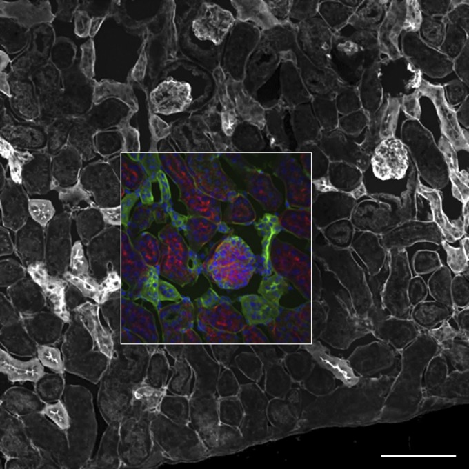
FOV comparison for an SDCM and a CLSM. A fixed mouse kidney section as in Fig. 1c, d was imaged with the same 20×/0.75 NA objective lens on a Yokogawa spinning-disk confocal equipped with a 512 × 512 pixel EM-CCD camera (inner square) and with the full FOV available on an Olympus FluoView 1000 CLSM (outer square; Tokyo, Japan). Scale bar, 100 μm.

Another limitation of the SDCM is that it does not have the same high-resolution sectioning ability along the z axis as the CLSM. The presence of multiple pinholes on the pinhole array disk results in out-of-focus light from other focal planes entering adjacent pinholes. This compromises z axis resolution and makes the SDCM inferior to the CLSM for z resolution. The effect is not so dramatic when imaging individual living cells in culture but may be prohibitive for thicker tissues or embryos. Most SDCMs have a fixed pinhole disk, with the pinhole size matched for maximal z axis resolution when using a 100× high-NA immersion objective lens. At lower magnifications, the pinholes are too large, so the optical-sectioning performance decreases. For example, when using a 10× objective on an SDCM, there is no major benefit when compared to a wide-field microscope. It is a mistake when users choose lower-magnification lenses to increase the SDCM FOV, resulting in poor optical-sectioning performance.

Most laser-based confocal microscopes (CLSM, RS-CLSM, and SDCM) use optical fibers to deliver the lasers into the microscope. For the laser-scanning confocals (CLSM and RS-CLSM), the laser power requirements are quite low (on the order of a few milliwatts) because all of the laser power is focused down to a single pixel in the specimen. However, for the SDCM, the laser power must be spread over the entire specimen FOV at once. For this reason, more powerful lasers, on the order of 25–50 mW per wavelength, are required. In addition, because the light output from the optical fiber has a Gaussian distribution, the FOV of the SDCM may be unevenly illuminated, with considerably higher intensity in the middle than at the edges of the FOV. This uneven illumination can be corrected for with postprocessing, and some manufacturers have come up with hardware solutions to minimize the nonuniformity.

final drawback of the SDCM is that multicolor applications can get complicated quickly with the need for multiple cameras, dichroic mirrors, and filter wheels. A single camera can be employed, and filter wheels can switch rapidly to excite and detect different fluorophores sequentially, but this precludes rapid acquisition of multiple probes. Alternatively, multiple cameras can be installed, but because the EM-CCD cameras are expensive ($30,000–$40,000), most systems are limited to 1 or 2 cameras. SDCMs do not inherently provide photomanipulation: the excitation laser light is not intense enough at any given focused laser spot for photoconversion, photoactivation, or significant photobleaching, and there is no inherent way to photomanipulate ROIs. However, a variety of separate laser-based systems for photomanipulation can be purchased for SDCMs, albeit with added cost and complexity.

New Developments

There are several new developments that directly address some of the shortcomings of the SDCM. The poor resolution and limited FOV of the SDCM may be addressed by installing new high-speed, high-sensitivity, and large FOV sCMOS cameras. These cameras boast a resolution of 4–5 megapixels (2048 × 2048 or 2560 × 2160), a QE of ∼70%, and due to parallel electronics on the camera chip, can record 100 high-resolution fluorescence images per second. Upgrading existing systems to sCMOS cameras is relatively straightforward. However, sCMOS cameras are not as sensitive and do not amplify signals in the same way as EM-CCD cameras; so they are not suited for many high-speed, low-light level applications. A nice compromise is that the SDCM can be equipped with 2 cameras: an EM-CCD camera for live-cell imaging of rapid cellular processes, and an sCMOS that can be used for live-cell imaging of slower biologic processes or for imaging of fixed specimens. Many manufacturers are now introducing SDCMs with variable pinhole sizes and pinhole spacing that are well matched for objective lenses of different magnifications and resolutions and can also reduce pinhole crosstalk. This option offers significant improvement when using the SDCM with lower-magnification objective lenses, improving the size of the FOV without compromising the optical-sectioning performance.

The uneven illumination on the SDCM is being addressed on some instruments through improved optics. For example, the Borealis illuminator from Spectral Applied Research (Richmond Hill, ON, Canada) changes the usual single-mode fiber for a larger-diameter multimode fiber, which delivers more light through to the microscope and also allows for a more-even illumination profile.

Finally, with high-powered diode lasers becoming increasingly affordable, the reduced efficiency in the excitation path of the SDCM is ameliorated by using brighter lasers (>100 mW) and bypassing Yokogawa’s microlens array. This allows manufacturers more flexibility in spinning-disk array design, pinhole size, pinhole spacing, and the use of novel disk designs. It also alleviates the need for the dichroic mirror to be sandwiched between the pinhole disk and the microlens disk, giving more flexibility in the design of the optical light path and for the addition of other optical components if they are needed. The emission path is unaffected, so the overall performance is similar to Yokogawa’s implementation. In addition, the high-power lasers can be used for other microscope techniques on the same microscope platform, such as total internal reflection fluorescence and/or single molecular localization superresolution microscopy.

CONCLUSIONS

In conclusion, there are many options when considering 3D confocal microscope platforms. The most basic form is the grid confocal that can be added to a wide-field microscope and can make use of the existing light source and camera. The grid confocal is affordable, but it is slow, insensitive, lacks high resolution, and is prone to noise and image artifacts. The SDCM is highly specialized to go fast. It is ideally suited for 3D live-cell imaging of 1–2 fluorescent probes in thin-to-moderately thick samples. It is also a much simpler microscope compared with the CLSM, so repairs and maintenance are more affordable. For high-speed applications, it has a limited FOV, lower resolution in x, y, and z, and is ideally suited for high-magnification immersion objective lenses. New developments in high-power lasers, camera technology, and versatile spinning-disk design show promise to bring the SDCM to other more general applications. The CLSM is by far the most versatile with multiple lasers, multiple detectors, a variable pinhole size, and the ability to adjust pixel size by simply controlling the laser-scanning precision. It can be optimized for applications with high or low magnification and with small or large specimens (i.e., small or large FOV). Resolution is high in x, y, and z, and multicolor applications are routine. The main pitfall of the CLSM is its slow speed. New CLSMs with both traditional and high-speed resonant-scanning mirrors nicely fill this gap, providing all of the benefits of the CLSM with the ability to image at high speed.

REFERENCES

- 1.Minsky M. Memoir on inventing the confocal scanning microscope. Scanning 1988;10:128–138. [Google Scholar]
- 2.White JG, Amos WB, Fordham M. An evaluation of confocal versus conventional imaging of biological structures by fluorescence light microscopy. J Cell Biol 1987;105:41–48. [DOI] [PMC free article] [PubMed] [Google Scholar]
- 3.Denk W, Strickler JH, Webb WW. Two-photon laser scanning fluorescence microscopy. Science 1990;248:73–76. [DOI] [PubMed] [Google Scholar]
- 4.Klar TA, Jakobs S, Dyba M, Egner A, Hell SW. Fluorescence microscopy with diffraction resolution barrier broken by stimulated emission. Proc Natl Acad Sci USA 2000;97:8206–8210. [DOI] [PMC free article] [PubMed] [Google Scholar]
- 5.Galdeen SA, North AJ. Live cell fluorescence microscopy techniques. Methods Mol Biol 2011;769:205–222. [DOI] [PubMed] [Google Scholar]
- 6.Goldman RD, Spector DL. Live Cell Imaging: A Laboratory Manual. Cold Spring Harbor Laboratory Press, NY, 2005. [Google Scholar]
- 7.Gräf R, Rietdorf J, Zimmermann T. Live cell spinning disk microscopy. Adv Biochem Eng Biotechnol 2005;95:57–75. [DOI] [PubMed] [Google Scholar]
- 8.Haraguchi T. Live cell imaging: approaches for studying protein dynamics in living cells. Cell Struct Funct 2002;27:333–334. [DOI] [PubMed] [Google Scholar]
- 9.Lacoste J, Vining C, Zuo D, Spurmanis A, Brown CM. Optimal conditions for live cell microscopy and raster image correlation spectroscopy. In Reviews in Fluorescence 2010. Geddes CD. (ed), New York: Springer; 2011:269–309. [Google Scholar]
- 10.Swedlow JR, Platani M. Live cell imaging using wide-field microscopy and deconvolution. Cell Struct Funct 2002;27:335–341. [DOI] [PubMed] [Google Scholar]
- 11.Zimmermann T, Rietdorf J, Pepperkok R. Spectral imaging and its applications in live cell microscopy. FEBS Lett 2003;546:87–92. [DOI] [PubMed] [Google Scholar]
- 12.Frigault MM, Lacoste J, Swift JL, Brown CM. Live-cell microscopy - tips and tools. J Cell Sci 2009;122:753–767. [DOI] [PubMed] [Google Scholar]
- 13.Lacoste J, Young K, Brown CM. Live-cell migration and adhesion turnover assays. In Cell Imaging Techniques, 3rd. (Taatjes DJ and Mossman BT (eds), Totowa, NJ: Humana Press, 2013:61–84. [DOI] [PubMed] [Google Scholar]
- 14.Nägerl UV, Willig KI, Hein B, Hell SW, Bonhoeffer T. Live-cell imaging of dendritic spines by STED microscopy. Proc Natl Acad Sci USA 2008;105:18982–18987. [DOI] [PMC free article] [PubMed] [Google Scholar]
- 15.Waters JC. Live-cell fluorescence imaging. Methods Cell Biol 2013;114:125–150. [DOI] [PubMed] [Google Scholar]
- 16.Nipkow P. Electric telescope, Patent no. 30105. Patented in the German Empire (Berlin) on January 6, 1884. Given January 15, 1885. [Google Scholar]
- 17.Petran M, Hadravsky M, Egger MD, Galambos R. Tandem-scanning reflected-light microscope. J Opt Soc Am 1968;58:661–664. [Google Scholar]
- 18.Art JJ, Goodman MB. Rapid scanning confocal microscopy. In Methods in Cell Biology, Brian M. (ed), New York: Academic Press, 1993:47–77. [DOI] [PubMed] [Google Scholar]
- 19.Langhorst MF, Schaffer J, Goetze B. Structure brings clarity: structured illumination microscopy in cell biology. Biotechnol J 2009;4:858–865. [DOI] [PubMed] [Google Scholar]
- 20.Neil MA, Juskaitis R, Wilson T. Method of obtaining optical sectioning by using structured light in a conventional microscope. Opt Lett 1997;22:1905–1907. [DOI] [PubMed] [Google Scholar]
- 21.Biggs DSC. Clearing Up Deconvolution, Pittsfield, MA: Biophotonics International, 2004. [Google Scholar]
- 22.Cannell MB, McMorland A, Soeller C. Image enhancement by deconvolution. In Handbook of Biological Confocal Microscopy, 3, Pawley J. (ed), New York: Springer, 2006:488–500. [Google Scholar]
- 23.Holmes TJ, Biggs D, Abu-Tarif A. Blind deconvolution. In Handbook of Biological Confocal Microscopy, 3, Pawley J. (ed), New York: Springer, 2006:468–487. [Google Scholar]
- 24.McNally JG, Karpova T, Cooper J, Conchello JA. Three-dimensional imaging by deconvolution microscopy. Methods 1999;19:373–385. [DOI] [PubMed] [Google Scholar]
- 25.Shaw P. Deconvolution in 3-D optical microscopy. Histochem J 1994;26:687–694. [DOI] [PubMed] [Google Scholar]
- 26.Shaw PJ. Comparison of widefield/deconvolution and confocal microscopy for three-dimensional imaging. In Handbook of Biological Confocal Microscopy, 3, Pawley J. (ed), New York: Springer, 2006:453–467. [Google Scholar]
- 27.Swedlow JR. Quantitative fluorescence microscopy and image deconvolution. Methods Cell Biol 2013;114:407–426. [DOI] [PubMed] [Google Scholar]
- 28.Wallace W, Schaefer LH, Swedlow JR. A workingperson’s guide to deconvolution in light microscopy. Biotechniques 2001;31:1076–1078, 1080, 1082 passim. [DOI] [PubMed] [Google Scholar]
- 29.Webb DJ, Brown CM. Epi-fluorescence microscopy. Methods Mol Biol 2013;931:29–59. [DOI] [PMC free article] [PubMed] [Google Scholar]
- 30.Wilson T. Optical sectioning in fluorescence microscopy. J Microsc 2011;242:111–116. [DOI] [PubMed] [Google Scholar]
- 31.Gustafsson MG. Surpassing the lateral resolution limit by a factor of two using structured illumination microscopy. J Microsc 2000;198:82–87. [DOI] [PubMed] [Google Scholar]
- 32.Hagen N, Gao L, Tkaczyk TS. Quantitative sectioning and noise analysis for structured illumination microscopy. Opt Express 2012;20:403–413. [DOI] [PMC free article] [PubMed] [Google Scholar]
- 33.Brown CM. Fluorescence microscopy—avoiding the pitfalls. J Cell Sci 2007;120:1703–1705. [DOI] [PubMed] [Google Scholar]
- 34.Cole RW, Jinadasa T, Brown CM. Measuring and interpreting point spread functions to determine confocal microscope resolution and ensure quality control. Nat Protoc 2011;6:1929–1941. [DOI] [PubMed] [Google Scholar]
- 35.Jonkman J, Brown CM, Cole RW. Quantitative confocal microscopy: beyond a pretty picture. Methods Cell Biol 2014;123:113–134. [DOI] [PubMed] [Google Scholar]
- 36.Murray JM. Practical aspects of quantitative confocal microscopy. Methods Cell Biol 2007;81:467–478. [DOI] [PubMed] [Google Scholar]
- 37.Waters JC. Accuracy and precision in quantitative fluorescence microscopy. J Cell Biol 2009;185:1135–1148. [DOI] [PMC free article] [PubMed] [Google Scholar]
- 38.North AJ. Seeing is believing? A beginners’ guide to practical pitfalls in image acquisition. J Cell Biol 2006;172:9–18. [DOI] [PMC free article] [PubMed] [Google Scholar]
- 39.Lippincott-Schwartz J, Altan-Bonnet N, Patterson GH. Photobleaching and photoactivation: following protein dynamics in living cells. Nat Cell Biol 2003;(Suppl):S7–S14. [PubMed] [Google Scholar]
- 40.Patterson GH. Photoactivation and imaging of photoactivatable fluorescent proteins. Curr Protoc Cell Biol 2008;38:21.6.1–21.6.10 [DOI] [PubMed] [Google Scholar]
- 41.Sheftel AD, Zhang AS, Brown C, Shirihai OS, Ponka P. Direct interorganellar transfer of iron from endosome to mitochondrion. Blood 2007;110:125–132. [DOI] [PubMed] [Google Scholar]
- 42.Yazawa M, Hsueh B, Jia X, Pasca AM, Bernstein JA, Hallmayer J, Dolmetsch RE. Using induced pluripotent stem cells to investigate cardiac phenotypes in Timothy syndrome. Nature 2011;471:230–234. [DOI] [PMC free article] [PubMed] [Google Scholar]
- 43.Digman MA, Brown CM, Horwitz AR, Mantulin WW, Gratton E. Paxillin dynamics measured during adhesion assembly and disassembly by correlation spectroscopy. Biophys J 2008;94:2819–2831. [DOI] [PMC free article] [PubMed] [Google Scholar]
- 44.Pawley J. Handbook of Biological Confocal Microscopy, New York: Plenum Press, 2006. [Google Scholar]
- 45.Zipfel WR, Williams RM, Webb WW. Nonlinear magic: multiphoton microscopy in the biosciences. Nat Biotechnol 2003;21:1369–1377. [DOI] [PubMed] [Google Scholar]
- 46.Cole RW, Thibault M, Bayles CJ, Eason B, Girard A-M, Jinadasa T, Opansky C, Schulz K, Brown CM. International test results for objective lens quality, resolution, spectral accuracy and spectral separation for confocal laser scanning microscopes. Microsc Microanal 2013;19:1653–1668. [DOI] [PubMed] [Google Scholar]
- 47.Borlinghaus RT. MRT letter: high speed scanning has the potential to increase fluorescence yield and to reduce photobleaching. Microsc Res Tech 2006;69:689–692. [DOI] [PubMed] [Google Scholar]
- 48.Nakano A. Spinning-disk confocal microscopy — a cutting-edge tool for imaging of membrane traffic. Cell Struct Funct 2002;27:349–355. [DOI] [PubMed] [Google Scholar]
- 49.Wilson T. Spinning-disk microscopy systems. Cold Spring Harbor Protocol, 2010:1208–1213. [DOI] [PubMed] [Google Scholar]
- 50.Maddox PS, Moree B, Canman JC, Salmon ED. Spinning disk confocal microscope system for rapid high-resolution, multimode, fluorescence speckle microscopy and green fluorescent protein imaging in living cells. Methods Enzymol 2003;360:597–617. [DOI] [PubMed] [Google Scholar]