Automated breast segmentation of fat and water MR images using dynamic programming

Abstract

Rationale and Objectives

To develop and test an algorithm that outlines the breast boundaries using information from fat and water magnetic resonance images.

Materials and Methods

Three algorithms were implemented and tested using registered fat and water magnetic resonance images. Two of the segmentation algorithms are simple extensions of techniques used for contrast-enhanced images: one algorithm uses clustering and local gradient (CLG) analysis; the other algorithm uses a Hessian-based sheetness filter (HSF). The third segmentation algorithm uses k-means++ and dynamic programming (KDP) for finding the breast pixels. All three algorithms separate the left and right breasts using either a fixed region or a morphological method. The performance is quantified using a mutual overlap (Dice) metric and a pectoral muscle boundary error. The algorithms are evaluated against three manual tracers using 266 breast images from 14 female subjects.

Results

The KDP algorithm has a mean overlap percentage improvement that is statistically significant relative to the HSF and CLG algorithms. When using a fixed region to remove the tissue between breasts with tracer 1 as a reference, the KDP algorithm has a mean overlap of 0.922 compared to 0.864 (<0.01) for HSF and 0.843 (<0.01) for CLG. The performance of KDP is very similar to tracers 2 (0.926 overlap) and 3 (0.929 overlap). The performance analysis in terms of pectoral muscle boundary error showed that the fraction of the muscle boundary within 3 pixels of reference trace 1 is 0.87 using KDP, compared to 0.578 for HSF and 0.617 for CLG. Our results show that the performance of the KDP algorithm is independent of breast density.

Conclusions

We developed a new automated segmentation algorithm (KDP) to isolate breast tissue from magnetic resonance fat and water images. KDP outperforms the other techniques that focus on local analysis (CLG and HSF) and yields a performance similar to human tracers.

INTRODUCTION

Breast density (BD) is a known risk factor for the development of breast cancer [1-4]. BD is routinely measured in mammography by comparing the ratio of stromal tissue to fatty tissue. Radiologists typically visually estimate BD from mammograms according to four categories: almost entirely fatty, scattered areas of fibroglandular densities, heterogeneously dense, or extremely dense [5]. Since increased BD (including the hetegeneously dense or extreme dense categories) is associated with a higher risk for breast cancer, therapies that reduce BD have been proposed as cancer preemptive treatments [6-8]. For studies assessing the effect of BD reduction therapies it is desirable to follow changes in BD longitudinally. Unfortunately, the radiation exposure in mammography makes the technique impractical for serial studies of BD. Mammograms also yield 2D information and the densities may change based on the projection, level and angle of compression, and scanner calibration [9].

Magnetic resonance imaging (MRI) is a non-invasive 3D imaging technique that uses non-ionizing radiation. More importantly, MRI yields distinct fat and water signals thus, the technique is an alternative to the mammographic measurement of BD. In recent years several MRI techniques have been developed for the measurement of fat-water content. These techniques are based on the acquisition of data where fat and water spins have different relative phases; the data are processed to reconstruct fat and water images corrected for the effect of field inhomogeneities [10-15]. In this study we use one of these techniques: the radial gradient- and spin-echo (RADGRASE) technique RADGRASE yields fat, water and T2-corrected fat-fraction (FF) images for the entire breast (approximately nineteen 7-mm thick slices) from data acquired in only three minutes [10]. Parameters derived from the FF distribution in the breast have showed a high correlation with mammography BD [16]. To analyze BD in the breast the first step is to define a region-of-interest (ROI) by segmenting the breast from the rest of the image. The manual segmentation of a stack of breast image slices is time consuming and impractical.

There has been an effort in developing breast segmentation algorithms. Oliver et al. [17] and Ganesan et al. [18] provide a review of different segmentation techniques developed for mammographic images. One review focuses on the segmentation of breast masses [17] while the other one examines different pectoral muscle boundary detection techniques [18]. There has been some work on the extraction of the breast ROI within breast MRI images as well. These algorithms mostly work with one type of image contrast (e.g., T1-weighted, T2-weighted images) to perform the segmentation [9,12,19-26] and are either semi-automated [19, 23-24] or need user-generated outlines to create statistical models [9,12,20]. Active contour models (i.e., snakes) have also been used for fully-automated breast image segmentation [21-22], however, the energy-optimization step can result in an unrealistic looking breast when there is not spatial continuity at the boundaries of the ROI. Giannini et al. [25] and Wang et al. [26] both developed fully automatic algorithms that do not require training data and are not based on active contours. Giannini et al. and Wang et al. both focus on dynamic contrast-enhanced images.

In this manuscript we describe a fully automated algorithm for the segmentation of breast images. The algorithm is based on a k-means++ [27] and dynamic programming [28] (KDP) approach and takes advantage of the different contrast in the fat and water images generated by fat-water imaging methods such as RADGRASE. The KDP algorithm was initially evaluated in only three subjects against one manual tracer using the Dice metric as the primary measure of performance [29]. Herein we assess the performance of the KDP algorithm in an expanded set of 14 subjects and compare the results to an algorithm based on clustering and local gradient (CLG) analysis and an algorithm that uses a Hessian-based sheetness filter (HSF), and we also compare to three trained manual tracers. The performance of the automated segmentation methods against manual tracers is evaluated using the Dice metric as well as a metric based on the correct delineation of the pectoral muscle boundary.

MATERIALS AND METHODS

Data Acquisition

The dataset consists of 266 axial breast slices corresponding to 14 female subjects (19 slices per subject) who were imaged as part of a research study at the Arizona Cancer Center. Out of the 266 breast slices, 172 were assigned to the “almost entirely fatty” BD category; 65 were assigned to the “scattered fibroglandular density” category, and 29 to the “heterogeneously dense” category. A breast radiologist performed the assignment by visually inspecting the MRI fat images.

RADGRASE data of the breast were acquired on a 1.5T GE Signal NV-CV/i scanner in the axial plane using a breast phased-array radiofrequency (RF) coil for signal detection. For fat-water separation, images were acquired using four gradient echoes per spin-echo, with phase shifts −5π/6,−π/6,π/2, and 7π/6, and receiver bandwidth of ±125 kHz. The echo train length (ETL) was 8 ms, and the TE range covered was of 11.5 – 89.3 ms; with these acquisition parameters the T2 contrast in the images was comparable to a TE ≈ 33 ms. Other parameters were: acquisition matrix size = 256 × 256, TR = 6 s, NEX = 1, FOV = 34 cm, and slice thickness = 7 mm. A saturation band was placed posterior to the pectoral muscle over the heart to reduce artifacts from cardiac motion. The acquisition of 19 slices took about 3 minutes. All subject identifiers were removed from the images prior to the segmentation study. Fat and water images were generated from the four gradient echo images as described in [10].

All human imaging studies were carried out with the approval of the local Institutional Review Board.

Automatic Segmentation Algorithm

Features in the Fat and Water Images

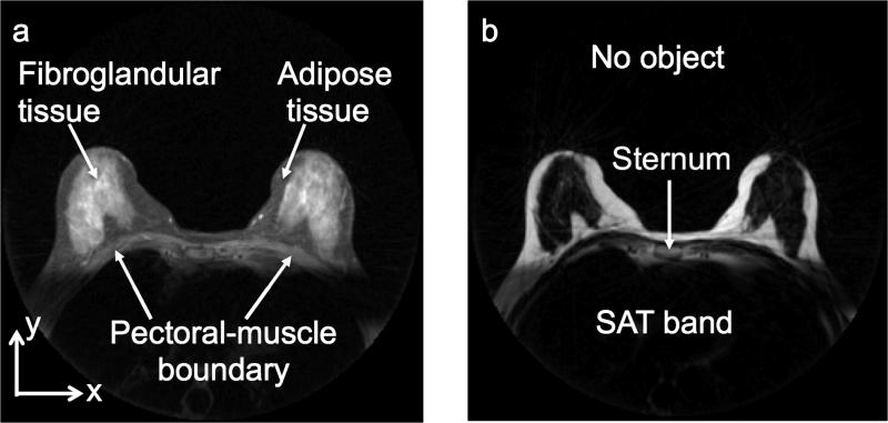
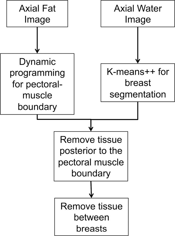
Typical water and fat images are shown in Figure 1. As can be seen from the figure, these two images have different contrast for the main components in breast tissue: the fibroglandular and the adipose tissues. In the water image, the fibroglandular tissue has high signal intensity compared to the adipose tissue, whereas in the fat image the contrast is reversed. The regions outside the breast that are important for segmentation purposes are also highlighted in Figure 1. The region outside the body habitus (the no-object region) has the lowest signal intensity in both images. The pectoral muscle (which separates the breast from the rest of the chest) has a signal intensity that is similar to that of the adipose tissue in the surrounding breast ROI in the water image. On average, the signal-to-noise ratio (SNR) of fibroglandular tissue, adipose tissue, and pectoral muscle in the water image is approximately 130, 45 and 55 dB, respectively. In the fat image the pectoral muscle has a lower signal intensity (SNR ≈ 7 dB) than the adipose tissue in the surrounding breast ROI (SNR ≈ 190 dB). In both images there is a rectangular region of low signal intensity below the pectoral muscle boundary due to the saturation (SAT) band, which was used to reduce the artifacts associated with cardiac motion. As will be shown below, KDP takes advantage of the contrast differences between these structures in the fat and water images for segmenting breast tissue from the rest of the chest. The stages of the segmentation algorithm are outlined in Figure 2.

Figure 1.

Axial (a) water and (b) fat images of the breast obtained from RADGRASE data.

Figure 2.

Schematic diagram of the segmentation algorithm.

Step 1: Initial Breast Segmentation

The first step in the algorithm is to eliminate most of the non-breast pixels using the water image. As can be seen in Figure 1a, the water image can be divided into three regions based on signal intensity: fibroglandular tissue (high signal intensity), adipose tissue and pectoral muscle (intermediate signal intensity), no object and SAT band (low signal intensity). The goal is to find a threshold that keeps the pixels with high and intermediate signal intensities and groups them into a single cluster. We use the k-means++ algorithm to cluster the image, although other methods such as Otsu or fuzzy C-means [30] can be used as well. The k-means++ algorithm is a variation of the original k-means algorithm where the centroids are not selected at random; instead, the probability of selecting a new centroid is proportional to its distance to existing centroids [27]. This reduces the probability of the k-means algorithm finding incorrect centroids.

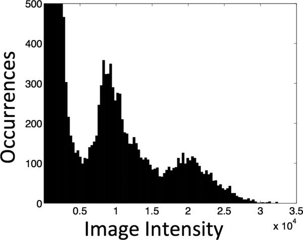
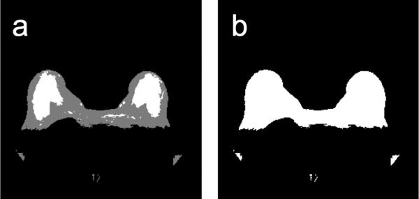
For this application, we group the pixels in the water image into three clusters (i.e., initialize three centroids). This number comes from analyzing the number of clusters found in multiple water images. Figure 3 is the histogram corresponding to the water image from Figure 1. The cluster with the lowest mean signal intensity contains the pixels associated with the no-object and SAT band regions; these pixels are eliminated from further processing. The cluster with intermediate mean signal intensity includes the pectoral muscle and adipose tissue pixels. Since we cannot differentiate between adipose tissue and pectoral muscle based on signal intensity, further refining is required. The cluster with high mean signal intensity contains the fibroglandular tissue pixels. The pixels corresponding to intermediate and high mean signal intensity clusters are used as an initial breast segmentation mask. The steps of the initial segmentation are illustrated in Figure 4.

Figure 3.

Histogram of the water image shown in Figure 1a (histogram was clipped for display purposes).

Figure 4.

Initial breast segmentation. (a) K-Means++ clustering of water image shown in Figure 1a using 3 clusters. (b) Initial breast segmentation mask.

Step 2: Pectoral Muscle Boundary Delineation

To refine the initial breast segmentation mask, we need to remove the pectoral muscle. If we look at the fat image (Figure 1b), there is a bright-to-dark transition at two tissue boundaries: the pectoral muscle-adipose tissue boundary and the adipose-fibroglandular tissue boundary. To automatically set up a starting point in the pectoral muscle tissue boundary, we focus on the sternum region, which includes the sternum and the adipose tissue around it. As explained below (see Step 3), the sternum region falls within the center of the image; thus, it is easy to locate automatically. We assume that there is no fibroglandular tissue in the sternum region; therefore, if a bright-dark transition is found, it is associated with the pectoral muscle-adipose tissue boundary, which we refer to as the pectoral muscle boundary. Once the starting point is determined, the pectoral muscle boundary is outlined by using the search technique known as dynamic programming. Dynamic programming in this context is a method that finds the minimum-cost 8-connected path (optimal path) between a starting and an ending pixel. Typical applications for dynamic programming include tracing vessels in medical images [28] and mammogram mass segmentation [31], among others.

The dynamic programming algorithm requires us to define a cost function. Let I_F(x,y) represent the fat image intensity at pixel (x,y). Using the coordinate system shown in Figure 1a, the cost function is defined as

$$C(x,y)=-\frac{d{I}_F(x,y)}{dy},$$

which is applied to the fat image (Figure 5a). This cost function outlines the bright-to-dark transitions in the fat image. A similar cost function was used by Giannini et al. [25] to find the pectoral muscle boundary. Using this cost function, the dynamic programming algorithm finds the minimum-cost path through the fat image, i.e., the path that maximizes the sum of the vertical derivatives values, $\frac{d{I}_F(x,y)}{dy}$, estimated in the discrete image using the well-known first-difference calculations I_F(x,y)−IF(x,y − 1). Dynamic programming requires a starting point which is set to the highest vertical derivative value in the sternum region, as described above. The path begins at the starting point and goes left and right, outlining the pectoral muscle boundary (Figure 5b). Since we know that the pixels posterior to the pectoral boundary are not part of the breast, we refine the initial breast segmentation mask (Figure 4b) by setting those pixels to 0 (Figure 5c).

Figure 5.

Pectoral muscle boundary extraction. (a) Cost function applied to the fat image shown in Figure 1b. (b) Pectoral muscle boundary (i.e., minimum-cost path). (c) Refined segmentation mask.

Step 3: Removing the Chest Tissue

In order to get individual ROIs for the left and right breasts, we need to remove the region in the chest that connects the breasts. Figure 1b shows that there is adipose tissue that is not part of the breast and is located in the sternum region. Using this information we proceed to remove any adipose tissue that falls inside the sternum region.

Aside from our initial implementation of KDP [29], we did not find any other method described in the literature to remove the sternum region. Therefore, in our analysis we used two methods. The first method is a fixed sternum removal (FSR) method, which removes all the adipose tissue in the fixed 29-column region centered within the sternum. In breast MRI the subject is always positioned on a breast RF coil which has a fixed geometry, so the center column of the image is within the sternum region. Thus, the region of 29 columns centered on the middle column of the image proved to be a good approach for removing the tissue between the breast given the 256 × 256 pixel resolution of our images. The second method is a morphological sternum removal (MSR) algorithm [29]. The MSR technique finds the smallest structuring element that removes most of the adipose tissue in the sternum region using morphological opening. To find the smallest structuring element, we find the number of pixels originally in the sternum region and see how the region is affected by doing a morphological opening on the refined initial breast segmentation mask. As the structuring element increases in size, the number of pixels left in the sternum region decreases. Since this behaves as a monotonically decreasing function, we can find the optimum structuring element by finding the knee in the curve. The knee of a curve is loosely defined as the point of maximum curvature [32]. The MSR method defines the knee as the point on the curve that is farthest from the line that connects the endpoints of the curve. Unlike FSR, the MSR method can adapt to different-sized sternum regions. Figure 6 shows examples of MSR and FSR applied to the mask of Figure 5d. By removing the adipose tissue not related to the breast, we are left with two breasts for analysis. The output of this module is the final breast segmentation mask, which is used for the performance analysis.

Figure 6.

Removal of tissue between the breasts. (a) Refined segmentation mask (from segmentation step 2). (b-c) Segmentation masks after removing the tissue between the breasts using the (b) fixed sternum removal (FSR) method and (c) morphological sternum removal (MSR) method.

Manual Tracing Protocol

The gold standard for the breast ROIs was manual tracing. The manual tracing protocol was determined by two experienced breast radiologists. The protocol for tracing the breast ROIs is as follows:

• The ROI contour is drawn on the water image, using the fat image as additional aid for areas where the border of the breast was not clear in the water image.

• To delineate precisely the anterior border of the breast, the brightness of the water image is increased to clearly see the noise signal in the no-object region.

• The starting point for delineating the anterior border of the breast ROI (i.e., the border between the adipose tissue and the no-object region) is determined by looking at the sternum region in the fat image. At the sternum, the anterior border is mostly horizontal, but as one moves transversally away from the sternum region, the anterior border starts to slope. The right and left points (from the central sternum region) where the anterior border starts to slope are considered the starting points for the anterior border of the right and left breast ROIs.

• Since the fat and water images are registered, each starting point is transferred to the water image, and the posterior border of the ROI is drawn, from those starting points, along the interface between the pectoral muscle and breast tissue. The brightness of the water image is reduced to a normal viewing level so that the pectoral muscle is discernible. The posterior border of the ROI is traced until the pectoral muscle tapers near the axilla. If the SAT band is reached before the end of the muscle, a straight horizontal line is drawn from that point in the image until reaching the border of the breast farthest from the midsaggital plane.

The tracing protocol was followed by the three tracers in the study (two radiologists and one non-radiologist trained to trace breast ROIs). In order to allow for human variability and biases in the manual tracing, each tracer was blinded to the others’ work. The automatic segmentation algorithm was designed in an effort to be consistent with this manual tracing protocol.

Extension of Other Algorithms to Fat-Water Images

We implemented a breast segmentation algorithm using clustering and local gradient analysis (CLG), which was derived from the algorithm by Giannini et al. [25]. Since their implementation is based on a single-contrast image (a dynamic contrast-enhanced MR image), we adapted the algorithm to work with the dual-contrast afforded by the fat and water images. The first step described in Giannini's algorithm is Otsu thresholding followed by morphological dilation. In our implementation we apply this first step on the water image. Giannini then finds the pectoral muscle boundary by applying a novel technique that maximizes local gradient difference. We apply this technique on the fat image. The refined initial breast segmentation mask is determined as the pixels between the breast/no-object boundary and the pectoral muscle boundary. Since Giannini's algorithm does not attempt to separate the breast ROI into left and right regions, we separated the resulting ROI using FSR and MSR. The output after separating the left and right breast ROIs is the final breast segmentation mask which is used for performance analysis.. The CLG algorithm yielded Dice metric values similar to the ones reported by Giannini [25].

We also implemented a Hessian-based sheetness filter (HSF) breast segmentation algorithm derived from the algorithm by Wang et al. [26]. The source code for Wang's algorithm was provided by those authors, and we adapted it to work with the fat and water images. The adaptation uses the water image to eliminate the SAT band and no-object pixels and uses the fat image to find the pectoral muscle boundary. The algorithm uses a Hessian-based sheetness filter scheme. The Hessian matrix is computed for each voxel (3D analysis), and the eigenvalues of that matrix are used to form a sheetness measure that provides a score from 0 to 1 indicating the likelihood that the voxel is located in a sheet-like neighborhood. Any voxel between the breast/no-object boundary and the pectoral muscle boundary is part of the refined initial breast segmentation mask. The final breast segmentation mask is obtained after applying the FSR or MSR method to split the left and right breast ROIs. The HSF algorithm yielded Dice metric values similar to the ones reported by Wang [26].

Performance Metrics

The performance analysis was based on two metrics: the Dice metric [33] and a row-wise difference between the automated and manually traced pectoral muscle boundary.

Dice Metric

The Dice metric computes the overlap between the ground truth and a segmented region:

$$\frac{2\mid X\cap Y\mid }{\mid X\mid +\mid Y\mid }.$$

In this equation X is the binary mask from manual segmentation and Y is the final breast segmentation mask. This metric gives an overall view of the segmentation quality, but due to its simplicity it can conceal important differences between boundaries. In spite of its drawbacks, it is a standard evaluation metric for segmentation algorithms [33].

Pectoral Muscle Boundary Difference

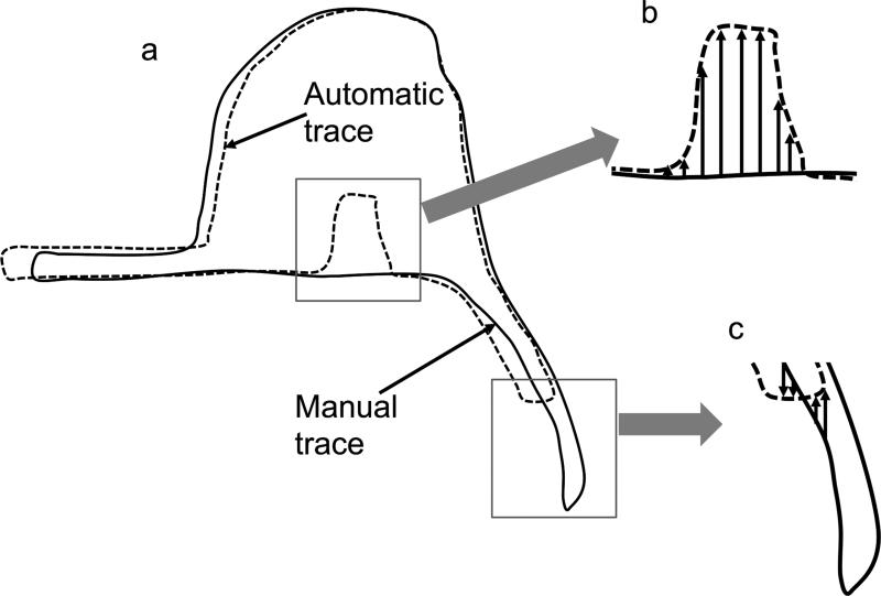
To compensate for one of the main drawbacks of the Dice metric, we wanted to find the difference in the pectoral muscle boundary between the automated traces and manual algorithms. Thus, within each column of data along the pectoral muscle boundary that appeared in both the automated and manual tracings, we computed the y-axis difference between the final breast segmentation mask (automatic trace) and the manual segmentation (manual trace). A schematic representation is shown in Figure 7. Note that we only focus the difference analysis on the posterior border of the mask because this boundary (associated with the pectoral muscle boundary) provides the biggest difference in performance between KDP and the other algorithms.

Figure 7.

Pectoral muscle boundary difference. (a) Schematic diagram of the manual and automatic tracings of a right breast ROI. (b) The y-axis difference between manual and automatic traces. (c) The y-axis difference only in columns where both traces are present.

Analysis Tools

Hypothesis Testing

To test whether the KDP algorithm is statistically better than the other automated algorithms, we used hypothesis testing to determine the confidence interval that will lead to the rejection of the null hypothesis. Our null hypothesis is that CLG and HSF have a higher mean accuracy than KDP. To account for the fact that the results of the algorithms are sampled, we apply Welch's two-sample t-test [33]. The t-statistic is computed as

$$t=\frac{{\mu }_1-{\mu }_2}{\sqrt{\frac{S_1^2}{N_1}+\frac{S_2^2}{N_2}}},$$

where μ₁ and s₁ are the mean and standard deviation of a first algorithm and μ₂ and S₂ are the mean and standard deviation of a second algorithm. For our experiments, the number of image slices analyzed is N₁ = N₂ = 266. A t-statistic of 2.34 would yield a p-value of 0.01, which indicates that μ₁ > μ₂ with 99% confidence (i.e., a one-tailed test).

Cumulative distribution function analysis

We used a cumulative distribution function (cdf) to compare performance between the different algorithms based on the pectoral boundary error. The cdf gives the probability that a discrete random variable has a value less than or equal to. Unlike hypothesis testing, the cdf analysis does not directly provide information regarding statistical significance information (e.g., p-value) but it does indicate the probability of achieving a desired performance level.

RESULTS

To compare the performance of the automated algorithms against the manual tracers using the Dice metric, we first analyzed the inter-tracer variability. Table 1 shows the results of the Dice metric analysis (mean and standard deviation based on a total of 266 slices) for the three manual tracers. We can see that even after following the tracing protocol (section 2.2), the percent overlap between the traces is in the low 90s. This reflects the variability between the manual tracers and serves as a usual reference when evaluating the performance of automated algorithms.

Table 1.

Inter-Tracer Performance (Dice Metric)

	Tracer #1		Tracer #2		Tracer #3
	μ *	σ †	μ	σ	μ	σ
Tracer #1	-	-	0.926	0.046	0.929	0.054
Tracer #2	0.926	0.046	-	-	0.902	0.070
Tracer #3	0.929	0.054	0.902	0.070	-	-

^*Mean value of the Dice metric

^†Standard deviation of the Dice metric

The next step was to compute the Dice metric between the automated algorithms and each of the manual traces. Table 2 shows the results of the Dice metric analysis for the two breast splitting techniques (FSR and MSR). Note that on average the KDP algorithm has a higher Dice mean and lower standard deviation than HSF and CLG. On average the FSR method yielded a higher Dice mean and lower standard deviation than MSR. Also note that the performance of KDP using FSR is within human variability. Looking at Table 1 and using tracer 2 as reference, one can see that the Dice mean values for tracers 1 and 3 are 0.926 and 0.902, respectively. As shown in Table 2, the Dice mean for KDP (with FSR) is 0.91 when compared to tracer 2. Table 3 applies hypothesis testing to the results in Table 2. Note that the-values are smaller than 0.01, meaning that there is 99% confidence that the KDP algorithm outperforms the other algorithms, regardless of the method used to remove the chest tissue between the breasts.

Table 2.

Automatic Segmentation Performance (Dice Metric)

Method	Splitting Technique	Tracer #1		Tracer #2		Tracer #3
		μ *	σ †	μ	σ	μ	σ
KDP	FSRM	0.922	0.047	0.910	0.052	0.908	0.067
	MSRM	0.897	0.114	0.878	0.123	0.899	0.107
HSF	FSRM	0.864	0.079	0.846	0.082	0.860	0.083
	MSRM	0.847	0.095	0.827	0.100	0.852	0.092
CLG	FSRM	0.843	0.107	0.830	0.109	0.835	0.119
	MSRM	0.833	0.113	0.817	0.121	0.831	0.119

^*Mean value of the Dice metric

^†Standard deviation of the Dice metric.

Table 3.

T-Score/P-Value Using Dice Metric

Methods	Splitting technique	Tracer #1		Tracer #2		Tracer #3
		t	p	t	p	t	p
KDP vs. HSF	FSRM	10.25	<0.01	10.60	<0.01	7.25	<0.01
	MSRM	5.49	<0.01	5.14	<0.01	5.44	<0.01
KDP vs. CLG	FSRM	11.00	<0.01	10.78	<0.01	8.69	<0.01
	MSRM	6.52	<0.01	5.70	<0.01	6.88	<0.01

Next we evaluated the performance of the automated algorithms using the pectoral muscle boundary difference. We used cdf analysis because the data does not have a normal distribution, so the t-test method will not yield reliable results. The cdf values presented in Table 4 show that for tracer 2, 84.8% of the pectoral muscle boundary pixels are within 3 pixels of the reference manual trace (tracer 1); for tracer 3 this percentage is 86.6%. For KDP using FSR, the percentage is 87.0%. For HSF and CLG, the percentages are 57.8% and 61.7%, respectively.

Table 4.

Pectoral Muscle Boundary CDF

Difference* (pixels)		0	≤1	≤2	≤3	≤4	≤5	≤10	≤20	≤50
Tracer #2	----	0.202	0.552	0.757	0.848	0.895	0.925	0.983	0.999	1.000
Tracer #3	----	0.253	0.624	0.797	0.866	0.901	0.926	0.981	0.998	1.000
KDP	FSRM	0.071	0.375	0.748	0.870	0.912	0.938	0.988	0.999	1.000
	MSRM	0.054	0.334	0.713	0.841	0.892	0.922	0.982	0.997	1.000
HSF	FSRM	0.025	0.159	0.438	0.578	0.631	0.671	0.828	0.967	1.000
	MSRM	0.019	0.140	0.419	0.567	0.625	0.666	0.820	0.959	0.999
CLG	FSRM	0.059	0.285	0.528	0.617	0.660	0.692	0.803	0.932	0.999
	MSRM	0.066	0.302	0.546	0.631	0.673	0.704	0.813	0.937	0.999

^*Difference in pixels from the pectoral boundary outline against a reference manual trace. The cdf is calculated by finding the percentage of the data that is equal or less than the difference values shown in the table.

The results show that the KDP performance is independent of BD. The Dice metric for the subsets assigned to the “almost entirely fatty” category (172 breast slices), “scattered fibroglandular density” category (65 breast slices), and “heterogeneously dense” category (29 breast slices) using the FSR splitting technique against tracer 1 are 0.91, 0.94 and 0.94, respectively. Using the same subset of breast images, we found that the percentages of the pectoral muscle boundary pixels that fall within 3 pixels of tracer 1 are 85.7%, 89.3% and 89.4%, respectively.

DISCUSSION

The results presented above show that KDP, which is based on k++ means clustering and dynamic programming using the contrast afforded by water and fat images, can be used for the automatic segmentation of breast images. In the analysis of 266 axial breast slices, the method outperformed two other methods derived from recently published segmentation algorithms and yielded ROIs of the left and right breast with Dice performance similar to manual tracers. The results show that segmentation performance is independent of BD.

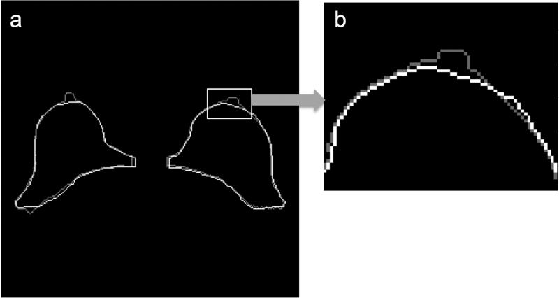
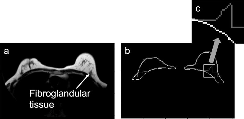
Despite its similarity to manual tracers, the KDP algorithm sometimes included regions that radiologists would not have included (e.g., the nipple). An example of a segmentation including the nipple is shown in Figure 8. The reason the nipple formed part of the breast segmentation mask is because its signal intensity in the water image is similar to the fibroglandular tissue. A way to eliminate the nipple is to find high curvature regions in the breast anterior boundary and eliminate them if they reside in the middle of the breast contour. If we look at the pectoral muscle boundary analysis (Table 4), we can see that there is a clear difference in performance between the HSF and CLG algorithms and KDP. Figure 9 illustrates the limitations of using algorithms that are based on local (i.e., HSF and CLG) rather than a global maximum (i.e., KDP). In Figure 9a, there is a region where the fibroglandular tissue is in direct contact with the pectoral muscle boundary (shown by the arrow), therefore eliminating the bright-to-dark transition feature that HSF and CLG rely upon to find the pectoral muscle boundary. Since both of these algorithms rely on a local algorithm to locate the boundary, they will select a bright-to-dark transition that may not be associated with the pectoral muscle boundary. Since KDP is based on cumulative analysis, it is able to find the correct location of the pectoral muscle boundary even if the bright-to-dark transition feature is not present in some areas.

Figure 8.

KDP outline (light gray) vs. manual trace outline (white). (a) Original outline. (b) Zoomed nipple region.

Figure 9.

Pectoral muscle boundary error. (a) Fat image indicating a region where the fibroglandular tissue is in direct contact with the pectoral muscle boundary (arrow). (b) Breast ROI outline according to [26] (light gray) vs. manually traced outline (white). (c) Zoomed pectoral muscle boundary.

Another part of the analysis evaluated the use of two different splitting techniques: FSR and MSR. The results show that FSR outperforms MSR in both performance metrics. In MSR, optimizing the morphological structuring element for individual slices allows flexibility in tracking subtle variation of the sternum region from one slice to the next, but it can sometimes go awry. On the other hand, FSR eliminates a fixed region in each slice; although this does not always identify the exact sternum region, it is a more consistent and well-defined process.

This work was performed using a combination of fat and water images generated by the RADGRASE technique, but it may be extended to other imaging techniques that yield registered fat and water images [10]. These include most of the phase-based chemical-shift MRI methods recently developed [10-15], where we expect similar differences in signal intensity between the tissues that are key for KDP segmentation (i.e., adipose, fibroglandular, and pectoral muscle tissues).

CONCLUSION

Based on the results shown, KDP is a practical option for the segmentation of fat and water breast images such as those generated by RADGRASE. Particularly encouraging is that the Dice accuracy using FSR (Table 2) was within human variability (Table 1). Moreover, KDP using FSR had 87.0% of its pectoral muscle boundary within three pixels of the reference tracer, whereas tracers 2 and 3 had 84.8% and 86.6% of the pectoral muscle boundary within three pixels of the reference tracer, respectively. In addition, the results show that KDP segmentation is independent of BD. For future work we wish to assess the performance of KDP using other fat-water imaging techniques and to extend the algorithm to other imaging modalities.

References

- 1.Wolfe JN. Risk for breast cancer development determined by mammographic parenchymal pattern. Cancer. 1976;5:2486–2492. doi: 10.1002/1097-0142(197605)37:5<2486::aid-cncr2820370542>3.0.co;2-8. [DOI] [PubMed] [Google Scholar]
- 2.Sandberg ME, Li J, Hall P, et al. Change of mammographic density predicts the risk of contralateral breast cancer - a case-control study. Breast Cancer Res. 2013;15:R57. doi: 10.1186/bcr3451. [DOI] [PMC free article] [PubMed] [Google Scholar]
- 3.Pinto Perreira SM, McCormack VA, Hipwell JH, et al. Localized fibroglandular tissue as a predictor of future tumor location within the breast. Cancer Epidemiol Biomarkers Prev. 2011;20:1718–1725. doi: 10.1158/1055-9965.EPI-11-0423. [DOI] [PMC free article] [PubMed] [Google Scholar]
- 4.McCormack VA, dos Santos Silva I. Breast density and parenchymal patterns as markers of breast cancer risk: a meta-analysis. Cancer Epidemiol Biomarkers Prev. 2006;15:1159–1169. doi: 10.1158/1055-9965.EPI-06-0034. [DOI] [PubMed] [Google Scholar]
- 5.Burnside ES, Sickles EA, Bassett LW, et al. The ACR BI-RADS experience: learning from history. J Amer Col Radiol. 2009;12:851–860. doi: 10.1016/j.jacr.2009.07.023. [DOI] [PMC free article] [PubMed] [Google Scholar]
- 6.Li J, Humphreys K, Eriksson L, et al. Mammographic density reduction is a prognostic marker of response to adjuvant tamofixen therapy in postmenopausal patients with breast cancer. J Clin Oncol. 2013;31:2249–2256. doi: 10.1200/JCO.2012.44.5015. [DOI] [PMC free article] [PubMed] [Google Scholar]
- 7.Cuzick J, Warwick J, Pinney E, et al. Tamoxifen-induced reduction in mammographic density and breast cancer risk reduction: a nested case-control study. J Natl Cancer Inst. 2011;103:744–752. doi: 10.1093/jnci/djr079. [DOI] [PubMed] [Google Scholar]
- 8.McTiernan A, Martin CF, Peck JD, et al. Estrogen-plus-progestin use and mammographic density in postmenopausal women: women's health initiative randomized trail. J Natl Cancer Inst. 2005;97:1366–1376. doi: 10.1093/jnci/dji279. [DOI] [PubMed] [Google Scholar]
- 9.Ortiz CG. M.S. thesis. Department of Medical Biophysics, University of Toronto; Toronto, Canada: 2011. Automatic 3D segmentation of the breast in MRI. [Google Scholar]
- 10.Li Z, Graff C, Gmitro AF, et al. Rapid water and lipid imaging with T2 mapping using a radial IDEAL-GRASE technique. Magnet Reson Med. 2009;6:1415–1424. doi: 10.1002/mrm.21918. [DOI] [PMC free article] [PubMed] [Google Scholar]
- 11.Clenden TV, Zeleniuch-Jacquotte A, May L, et al. Comparison of 3-point Dixon imaging and fuzzy C-means clustering methods for breast density measurement. J Magn Reson Im. 2013;38:474–481. doi: 10.1002/jmri.24002. [DOI] [PubMed] [Google Scholar]
- 12.Wang Y, Morrell G, Heibrun ME, et al. 3D multi-parametric breast MRI segmentation using hierarchical support vector machine with coil sensitivity correction. Acad Radiol. 2013;20:137–147. doi: 10.1016/j.acra.2012.08.016. [DOI] [PMC free article] [PubMed] [Google Scholar]
- 13.Ma JF, Son JB, Zhou Y, et al. Fast spin-echo triple-echo Dixon (fTED) technique for efficient T2-weighted water and fat imaging. Magn Reson Med. 2007;58:103–109. doi: 10.1002/mrm.21268. [DOI] [PubMed] [Google Scholar]
- 14.Bley TA, Wieben O, Francois CJ, et al. Fat and water magnetic resonance imaging. J Magn Reson Im. 2010;31:4–18. doi: 10.1002/jmri.21895. [DOI] [PubMed] [Google Scholar]
- 15.Madhuranthakam AJ, Yu H, Shimakawa A, et al. T(2)-weighted 3D fast spin echo imaging with water-fat separation in a single acquisition. J Magn Reson Im. 2010;32:745–751. doi: 10.1002/jmri.22282. [DOI] [PMC free article] [PubMed] [Google Scholar]
- 16.Trouard TP, Thompson P, Huang C, et al. Fat water ratio and diffusion-weighted MRI applied to the measure of breast density as a cancer risk biomarker. Proc Int Soc Magn Res Med. 2010:4749. [Google Scholar]
- 17.Oliver A, Freixenet J, Martí J, et al. A review of automatic mass detection and segmentation in mammographic images. Med Image Anal. 2010;2:87–110. doi: 10.1016/j.media.2009.12.005. [DOI] [PubMed] [Google Scholar]
- 18.Ganesan K, Acharya UR, Chua KC, et al. Pectoral muscle segmentation: a review. Comput Meth Prog Bio. 2013;1:48–57. doi: 10.1016/j.cmpb.2012.10.020. [DOI] [PubMed] [Google Scholar]
- 19.Nie K, Chen JH, Chan S, et al. Development of a quantitative method for analysis of breast density based on three-dimensional breast MRI. Med Phys. 2008;12:5253–5262. doi: 10.1118/1.3002306. [DOI] [PMC free article] [PubMed] [Google Scholar]
- 20.Ertas G, Gulcur H, Osman O, et al. Breast MR segmentation and lesion detection with cellular neural networks and 3D template matching. Comput Biol Med. 2008;1:116–126. doi: 10.1016/j.compbiomed.2007.08.001. [DOI] [PubMed] [Google Scholar]
- 21.Kass M, Witkin A, Terzopoulos D. Snakes: active contour models. Int J Comput Vision. 1988;4:321–331. [Google Scholar]
- 22.Xu C, Prince JL. Snakes, shapes, and gradient vector flow. IEEE T Image Process. 1998;3:359–369. doi: 10.1109/83.661186. [DOI] [PubMed] [Google Scholar]
- 23.Lee N, Rusinek H, Weinreb J, et al. Fatty and fibroglandular tissue volumes in breasts of women 20-83 years old: comparison of X-ray mammography and computer-assisted MR imaging. Am J Roentgenol. 1997;2:501–506. doi: 10.2214/ajr.168.2.9016235. [DOI] [PubMed] [Google Scholar]
- 24.Khazen M, Warren RML, Boggis CRM, et al. A pilot study of compositional analysis of the breast and estimation of breast mammographic density using three-dimensional T1-weighted magnetic resonance imaging. Cancer Epidem Biomar. 2008;9:2268–2274. doi: 10.1158/1055-9965.EPI-07-2547. [DOI] [PMC free article] [PubMed] [Google Scholar]
- 25.Giannini V, Vignati A, Morra L, et al. A fully automatic algorithm for segmentation of the breast in DCE-MR images. Proc Eng Med Biol Soc. 2010:3146–3149. doi: 10.1109/IEMBS.2010.5627191. [DOI] [PubMed] [Google Scholar]
- 26.Wang L, Platel B, Ivanovskaya T, et al. Fully automatic breast segmentation in 3D breast MRI. Int Symp Biomed Imaging. 2012:1024–1027. [Google Scholar]
- 27.Arthur D, Vassilvitskii S. K-means++: the advantages of careful seeding. Proc Eighteenth Annu Assn Comput Mach Soc Ind Appl Math, Symp Discrete Alg. 2007:1027–1035. [Google Scholar]
- 28.Sonka M, Hlavac V, Boyle R. Segmentation I. In: Sonka M, Hlavac V, Boyle R, editors. Image Processing, Analysis and Machine Vision. Global Engineering; Stanford, CT: 2014. pp. 206–210. [Google Scholar]
- 29.Rosado-Toro JA, Barr T, Galons JP, et al. Automated segmentation of breast fat-water MR imaging using empirical analysis. IEEE Int Conf Acoust Speech Signal Process. 2013:1018–1022. [Google Scholar]
- 30.Pal NR, Bezdek JC. On cluster validity for the fuzzy c-means model. IEEE T Fuzzy Syst. 1995;3:370–379. [Google Scholar]
- 31.Timp S, Karssemejier N. A new 2D segmentation method based on dynamic programming applied to computer aided detection in mammography. Med Phys. 2004;5:958–971. doi: 10.1118/1.1688039. [DOI] [PubMed] [Google Scholar]
- 32.Salvador S, Chan P. Determining the number of clusters/segments in hierarchical clustering/segmentation algorithms. ICTAI. 2004:576–584. [Google Scholar]
- 33.Dice L. Measures of the amount of ecologic association between species. Ecology J. 1945;3:297–302. [Google Scholar]
- 34.Yuen KK. The two-sample trimmed t for unequal population variances. Biometrika. 1974;1:165–170. [Google Scholar]