Abstract
Purpose:
Transverse relaxation analysis with several signal models has been used extensively to determine tissue and material properties. However, the derivation of corresponding parameter values is notoriously unreliable. We evaluate improvements in the quality of parameter estimation using Bayesian analysis and incorporating Rician noise, as appropriate for magnitude MR images.
Theory and Methods:
Monoexponential, stretched exponential, and biexponential signal models were analyzed using nonlinear least squares (NLLS) and Bayesian approaches. Simulations, and phantom and human brain data, were analyzed using three different approaches to account for noise. Parameter estimation bias, reflecting accuracy, and dispersion, reflecting precision, were derived for a range of signal-to-noise ratios (SNR) and relaxation parameters.
Results:
All methods performed well at high SNR. At lower SNR, the Bayesian approach yielded parameter estimates of considerably greater precision, as well as greater accuracy, than did NLLS. Incorporation of Rician noise greatly improved accuracy and, to a somewhat lesser extent, precision, in derived transverse relaxation parameters. Analyses of data obtained from solution phantoms and from brain were consistent with simulations.
Conclusion:
Overall, estimation of parameters characterizing several different transverse relaxation models was markedly improved through use of Bayesian analysis and through incorporation of Rician noise.
Keywords: Bayesian probability, Nonlinear least squares algorithm, Transverse relaxation, Brain, Accuracy, Precision, Rician noise
INTRODUCTION
Relatively little work has been undertaken to evaluate the Bayesian probability approach to parameter estimation from noisy MR images. In particular, the performance of Bayesian as compared to nonlinear least squares (NLLS) analysis in the quantification of transverse decay, as described by monoexponential and alternative models, has not been reported. However, these models are of increasing interest in both preclinical and clinical studies in order to characterize tissue ultrastructure, identify tissue compartments, and differentiate between normal and pathologic tissues.
Multiexponential transverse relaxation analysis (METRA) (1-7) is one approach to this type of characterization, in which extraction of transverse relaxation times and component amplitudes from relaxation data is achieved through use of the inverse Laplace transform (ILT). This is typically implemented through the NLLS or the nonnegative least square algorithms. However, the ill-posed nature of the ILT makes the inversion very sensitive to noise (8-9), rendering parameter estimation difficult, especially in the clinical setting.
It has been demonstrated that explicitly incorporating the Rician noise model appropriate to magnitude magnetic resonance (MR) images (10-11) greatly improves accuracy and precision in derived parameter estimates (12-14), including for biexponential signals (15). Despite this, bias and dispersion resulting from application of NLLS increase substantially with decreasing SNR or with increasing disparity between component sizes (15-16).
Parameter estimation using Bayesian probability theory has long been recognized as having several advantages over NLLS minimization (17-18), including the fact that it does not require initial estimates. In addition, the estimate of a given parameter is derived through integration, or marginalization, over the probability distribution functions (PDFs) of the remaining parameters. The resulting PDF of the parameter of interest, the so-called posterior PDF, is therefore not influenced by local minima of a global fitting function defined by multiple parameters as is the case for NLLS (19). The posterior PDF completely defines the uncertainty in the derived parameter estimate (20). Among other benefits, this permits assessment of MR parameter uncertainty within a single voxel (21).
While laying a foundation for Bayesian analyses of MR data, these previous results were restricted to NMR spectroscopic data or to monoexponential transverse decay over a restricted parameter range. In the present work, our goal is to provide a much more comprehensive evaluation of the quality of parameter estimation from transverse relaxation imaging data through use of Bayesian analysis as compared to NLLS. Analyses were performed using the appropriate Rician noise model, as that has been clearly demonstrated to provide improved estimates as compared to the Gaussian noise approximation (12-15, 21). Three distinct signal relaxation models were studied, the monoexponential, stretched exponential, and biexponential, over a large range of parameters and SNR values. All three of these models are used in the analysis of complex systems.
We first review the theory of noise distribution in MR images. We then describe in detail the six different voxel-by-voxel fitting methods we compared, three based on NLLS minimization and three based on Bayesian analysis. Next, extensive Monte Carlo (MC) simulations are presented which give the relative bias and dispersion in the estimation of transverse relaxation parameters using the six methods. Finally, we present data obtained from phantoms at 7 Tesla (T) and from human brain at 3T.
THEORY
MRI Signal Distribution
The PDF of magnitude imaging data S = {Sn} measured at echo times TEn = n * TE defined by echo time TE and echo number n, with Gaussian-distributed noise of equal variance, σ2, in the real and imaginary channels, is given by the Rician distribution (10):
| [1] |
where A(θ;TEn), is the magnitude of the underlying noise-free signal as a function of TEn and signal parameters θ, Ik is the modified k-order Bessel function of the first kind and u is the Heaviside step function. The first moment, or expectation value, of the Rician PDF is given by (22-23)
| [2] |
where φn = A2(θ;TEn)/2σ2.
From Eq. 1, the likelihood function for the transverse decay data within a voxel is (24)
| [3] |
At high SNR, SnA(θ;TEn) » σ2 so that I0(A(θ;TEn)Sn/σ2) approaches . In this limit, the Rician PDF approximates the Gaussian distribution with mean A(θ;TEn) and variance σ2 (11, 25):
| [4] |
with first moment, or expectation value, given by
| [5] |
From Eq. 4, the Gaussian likelihood function of the imaging data S is
| [6] |
NLLS and Bayesian Parameter Estimation Approaches
NLLS parameter estimation is generally rapid and accurate for low dimensional problems, that is, those for which the number of parameters to be estimated is small. However, in higher dimensions, NLLS estimation is greatly complicated by the presence of local minima; this difficulty increases with model complexity, with an increasing number of free parameters to be determined, and with decreasing SNR (19).
Bayesian analysis is an alternative approach that can be particularly robust for parameter estimation in the presence of noise (17, 20-21, 26-34). In this framework, parameter probability distributions are calculated from the observed data and prior knowledge. Bayesian parameter estimation is based on the posterior probability density of parameters, θ, given the observed data, S, and the standard deviation of the noise, σ. The formal statement of Bayes theorem in this context is (35-36):
| [7] |
where P(θ) represents an a priori parameter distribution based on pre-existing knowledge, L(S|θ,σ) is the likelihood function of S given θ and σ, and P(S) is a normalization constant, which corresponds to our use of normalized probability distributions.
The successive marginalization over all parameters results in a considerable computational burden, but permits the calculation of a posterior PDF for each individual parameter. An estimate can be derived from the PDF of θi in several ways. It can be taken as the mean of the PDF P(θi|S,σ), as is widely used in statistical inference, or as its median value. In this paper, we define as the maximum posterior probability (MAP), as is common in Bayesian image analysis (37):
| [8] |
METHODS
Transverse Relaxation Signal Models
Monoexponential Signal
The monoexponential model implicitly assumes a single pool of water protons, leading to transverse decay of the form:
| [10] |
Thus, this model is characterized by the parameter pair θ = (A0 T2), with A0 representing the signal amplitude for TE = 0, incorporating T1-weighting, proton density, coil sensitivity and other machine factors. T2 represents the spin-spin relaxation time.
Stretched Exponential Signal
Biological tissues are characterized by a complex physicochemical structure (1-7, 38-41) so that the monoexponential function (Eq. 10), while often a useful approximation, would not be expected to account for important features of transverse relaxation (42). Therefore, alternative relaxation models that permit a more detailed description of the relationship between relaxation or diffusion processes and internal material structure have become of interest (43-47).
The stretched exponential decay model is given by
| [11] |
with parameters θ = (A0 g=a T2; α ∈ (0,1] defines the deviation from monoexponential decay. This arises in several settings, including as an approximation to a continuous distribution of decay constants and in systems with memory as represented by fractional order processes (47).
Biexponential Signal
Restricting METRA to biexponential signals has been found to be a good approximation to transverse relaxation in a number of studies and is particularly appropriate in settings of only moderate SNR, such as is achievable clinically (48-51). For the case of two distinct proton pools that are not exchanging, the signal decay function is
| [12] |
with parameters θ = (A0fsT2,sT2,l), where fs is the fraction of the short T2 component, and T2,s and T2,l are the spin-spin relaxation times of the short-T2 and long-T2 components, respectively. It is well-known that derivation of accurate parameter values can be highly problematic (15-16) even for this simple biexponential signal model.
Parameter Estimation Methods
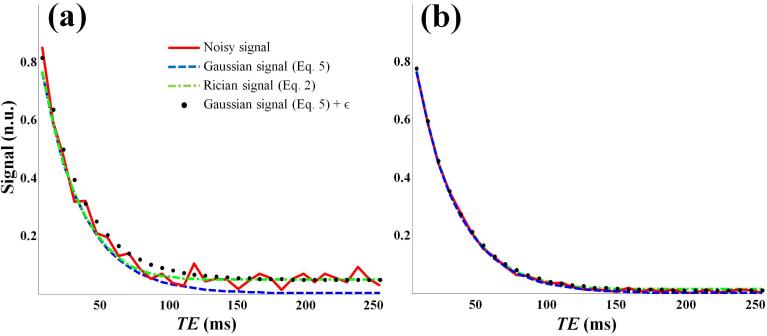
For each of the above three signal models, six methods of parameter estimation were implemented. They are defined by use of NLLS versus Bayesian analysis, and by signal models using Gaussian noise, Gaussian noise plus an offset, and Rician noise. More precisely, the first method, denoted NLLSG, uses the Gaussian estimator in Eq. 5, and consists of NLLS minimization of Sn − EGauss[Sn], that is, Sn − A(θ;TEn), with A(θ;TEn) defined by Eqs. 10-12. The second method evaluated, NLLSG,O, uses the Gaussian estimator plus an offset ε, and consists of NLLS minimization of Sn − (A(θ;TEn) + ε). This is the simplest method used to account for noise in magnitude reconstruction (52-54) (Fig. 1). The third method, NLLSR, makes full use of the expectation value of the Rician distribution given by Eq. 2, and involves NLLS minimization of Sn − ERice[Sn]. The fourth method, MAPG, is a Bayesian analysis using the Gaussian likelihood function, LGauss(S|θ,σ), given by Eq. 6. The fifth parameter estimation method, MAPG,O, is a Bayesian analysis using the Gaussian likelihood function, LGauss(S|θ,σ), given by Eq. 6, but incorporating an offset, so that (A(θ;TEn) is replaced by (A(θ;TEn). The sixth method evaluated, MAPR, is a Bayesian analysis using the Rician likelihood function, LRice(S|θ,σ), given by Eq. 3. The marginalization process required in the Bayesian-based methods is described in the Appendix. All numerical calculations were performed using Matlab (MathWorks, Natick, MA, USA), with NLLS fits performed with the Levenberg-Marquardt algorithm.
Fig. 1.
Signals as a function of TEn generated for T2 = 30 ms and A0 = 1, assuming monoexponential transverse decay (Eq. 10) with SNR of 20 (Panel a) and 100 (Panel b). The noisy signal, S(TEn), was obtained through addition of Rician noise to the underlying noise-free signal,A(θ;TEn), according to where the noise in the real and imaginary channels, Nre and Nim, was generated from a Gaussian distribution with zero mean and standard deviation σ.
Estimations of Standard Deviation, Variance and Offset of the Noise
We take the standard deviation, σ, variance, σ2, and offset, ε, of the noise as known parameters. These were input values in our simulation studies, while in phantom and in vivo studies they were estimated from background regions in which A(θ;TEn) = 0 so that Eq. 1 reduces to the Rayleigh distribution (11, 55-56):
| [13] |
The first and the second moments of PRayleigh(Sn|σ) are (57-58)
| [14] |
and
| [15] |
from which unbiased estimates of σ, σ2 and ε may be obtained through (57-58), where K is the total number of voxels taken as background. Note that to improve the quality of these estimates, the signal-free regions were formed from the background intensity in all of the echo images.
Bias and Dispersion Calculations
For each method, the relative bias, a measure of accuracy, was defined from the difference between the true value, θi, and the mean of the estimated value, , by . In simulations, M is the total number of noise realizations, while in phantom studies it is the total number of voxels for which parameter maps were generated. In simulations, true parameter values were known, while in phantom studies they were obtained from a monoexponential fit (12) of high SNR data acquired from each phantom compartment separately (see below). Note that the phantom studies were limited to the monoexponential and biexponential models. Relative dispersion, a measure of precision, was similarly defined by
Relative bias and dispersion were calculated after removal of voxels with extreme outliers (VEO) using Tukey’s method (59) to correspond to actual practice (12, 15).
In contrast to simulations and phantom studies, exact parameter values for the brain were unknown so that relative bias and dispersion cannot be evaluated. Instead, relative error maps for each estimated parameter were calculated using MAPR analysis of high SNR imaging data as the reference, although we note that maps were essentially identical for all analysis methods using the high SNR data. For each estimated parameter, errors in the values obtained at lower SNR were calculated from the difference between the estimated value, , and its reference value, , according to .
In simulations, SNR was defined as A(θ;TEn)/σ, where TE1 is the shortest echo time at which data were generated. In phantom and in vivo studies, it was defined as (60), where S̄(TE1) represents the mean signal calculated from a large region of the MR image obtained at TE1.
Numerical Simulation Studies
MC simulations were performed using monoexponential (Eq. 10), stretched exponential (Eq. 11), and biexponential (Eq. 12) signal models for a wide range of underlying parameters and as a function of SNR, achieved through addition of Rician noise (Fig. 1). For all simulations, a total of 32 data points were generated with TEn increasing uniformly from 8 to 256 ms. The required starting values needed in the NLLS analyses were set to their true values. For each signal model and for each set of parameters, relative bias and dispersion were calculated over 1000 noise realizations for each estimated parameter using the six analysis methods.
MC Simulations 1: Effect of SNR
MC simulations were performed to examine the effect of SNR on the relative bias and dispersion in derived parameters. The underlying true model parameters were chosen to reflect values obtained from the in vivo study of human brain (below).
For the monoexponential (Eq. 10), T2 = 70 ms was used, with Rician noise added to achieve SNR ranging from 10 to 60 in increments of 10. For the stretched exponential (Eq. 11), T2 = 60 ms and α = 0.8 were used, with SNR values ranging from 10 to 100 in increments of 10. For the biexponential analysis (Eq. 12), the underlying parameters were fs = 0.25, T2,s = 20 ms and T2,l = 90 ms, with an SNR range of 30 to 120, again in increments of 10. The different SNR ranges were selected to account for the difference in complexity of these three signal models. For example, the SNR requirement for the monoexponential is less stringent than for the other two models, so lower values of SNR were appropriate for the analysis. The parameter estimates begin to break down severely at the lower limit of SNR, and became relatively stable at the higher value, in each case.
MC Simulations 2: Effect of Underlying Parameters
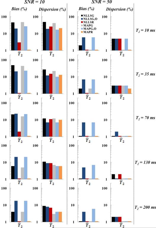
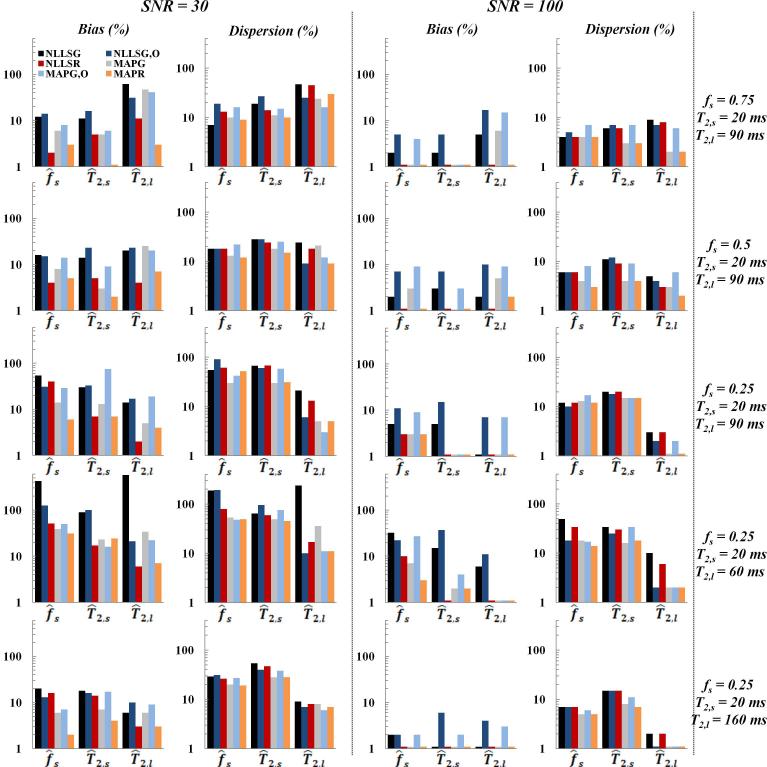
MC simulations were also used to explore the effect of underlying true parameter values on the relative bias and dispersion in derived parameters. The wide range of underlying parameters investigated is summarized in Fig. 3-5. Again, appropriate values of SNR were selected, with SNR of 10 and 50 for the monoexponential, 10 and 70 for the stretched exponential, and 30 and 100 for the biexponential.
Fig. 3.
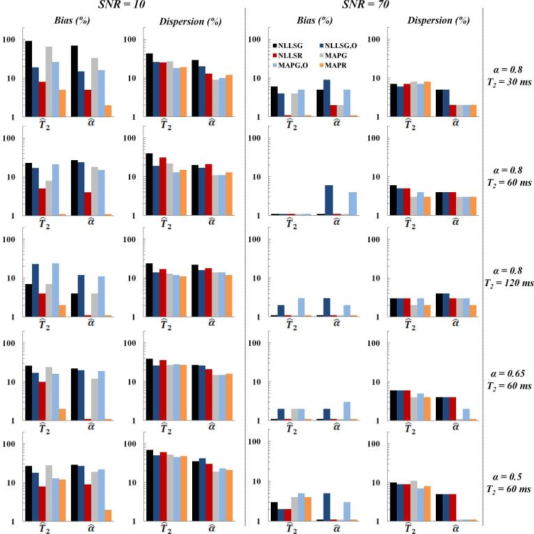
Relative bias and dispersion in T2 estimates obtained using Monte Carlo simulations for the monoexponential signal model at SNR of 10 (left column) and 50 (middle column) using the NLLSG, NLLSG,O, NLLSR, MAPG, MAPG,O and MAPR analysis methods for five different input T2 values (right column). Decreased bias and dispersion, that is, improved accuracy and precision, were achieved through use of Rician noise model and Bayesian analysis as discussed in detail in the text.
Fig. 5.
Relative bias and dispersion of the estimates of fs, T2,s and T2,l obtained using Monte Carlo simulations for the biexponential signal model at SNR of 30 (left column) and 100 (middle column) using NLLSG, NLLSG,O, NLLSR, MAPG, MAPG,O and MAPR analysis methods for five different combinations of fs, T2,s and T2,l (right column). Decreased bias and dispersion, that is, improved accuracy and precision, were achieved through use of Rician noise model and Bayesian analysis as discussed in detail in the text.
Phantom Studies
Phantom studies were designed to validate the monoexponential and biexponential MC simulations. Three rectangular tubes (5 × 3 cm) filled with deionized water were doped with different concentrations of CuSO4. The tubes were then placed together in the MRI system, and images were acquired using a 3D CPMG sequence (61-62) on a 7T small animal MRI scanner (Bruker Biospin GmbH, Rheinstetten, Germany) equipped with a linearly polarized birdcage coil. 35 T2-weighted images with TEn increasing linearly from 5.1 to 180 ms were acquired. Other imaging parameters included TR = 1000 ms, field of view (FOV) = 70 × 40 × 40 mm3, and matrix = 140 × 80 × 20. Images were obtained with different numbers of signal averages, ranging from 1 to 8. Linear combinations of complex imaging data from each pair of phantoms were created and added with consistent phases to obtain Rician-distributed magnitude images with different compartment fractions (15). Relative bias and dispersion were calculated for each estimated parameter using the six analysis methods. Fiducial T2 values were obtained from high SNR data acquired from each tube independently and fit to a monoexponential; they were 14 ± 2 ms, 58 ± 1 ms and 112 ± 3 ms from tubes 1, 2 and 3, respectively. These were used as initial estimates for the NLLS analysis.
Phantom Study 1: Effect of SNR
Images acquired from tube 2, with T2 = 58 ms, were fit to a monoexponential using the six investigated methods. Data from the separate measurements on tube 1, with T2 = 14 ms, and tube 3, with T2 =112 ms, were constructed as described above in order to synthesize two-component images with fs = 0.33 and with a range of SNR's. Each voxel from these composite images was fit to a biexponential function.
Phantom Study 2: Effect of Underlying Parameters
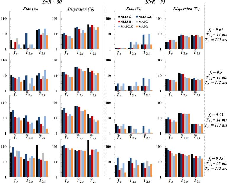
T2 weighted images were fit to a monoexponential independently for each of the three imaged tubes. For the biexponential, different composite images were created with several fs values and ratios T2,l/T2,s (see Fig. 8). Fits were performed at two different SNR's, as indicated in Fig. 8.
Fig. 8.
Relative bias and dispersion obtained from phantom measurements for the estimation of fs, T2,s and T2,l, with a biexponential signal model, for SNR of ~ 30 (left column) and ~ 95 (middle column), using NLLSG, NLLSG,O, NLLSR, MAPG, MAPG,O and MAPR analysis methods, for four different combinations of input fs, T2,s and T2,l values (right column). Improvements in accuracy and precision are seen through use of Rician noise model and Bayesian analysis, as discussed in the text.
In vivo Study
T2-weighted images of the brain of a 40 year-old male volunteer were acquired with a 3T whole-body MRI system (Achieva, Philips Medical Systems) equipped with a quadrature head coil. 32 axial MR images were obtained using a 3D CPMG sequence with TEn increasing linearly from 8 to 256 ms, TR = 700 ms, FOV = 240 × 240 × 15 mm3 and matrix = 320 × 240 × 5. Images were obtained for different numbers of signal averages to vary SNR. Data were fit to monoexponential, stretched exponential and biexponential functions using the six methods investigated. Relative error maps were then calculated as described above in the "Bias and Dispersion Calculations" section. Parameter values obtained at the highest SNR were used as starting values for the NLLS-based methods.
RESULTS
Numerical Simulation Studies
Results of the MC simulations were obtained after removal of VEO. The number of removed VEO was almost identical among the six methods, and was less than 1% at the larger, though still moderate, SNR for each. Even at the lower SNR, corresponding to truly modest image quality, VEO represented only a relatively small fraction of the total voxels. Less than 2% of the voxels were excluded for the monoexponential, less than 5% for the stretched exponential, and less than 8% for the biexponential.
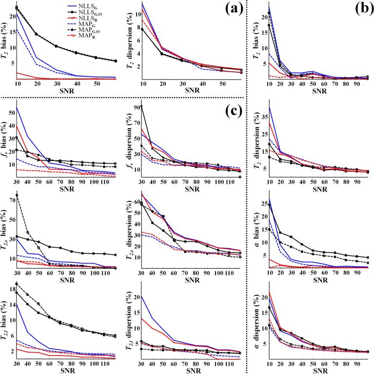
Fig. 2 shows the relative bias, as a measure of accuracy, and the relative dispersion, as a measure of precision, in parameter estimates for the monoexponential, with T2 as the fit parameter of interest (Fig. 2a), the stretched exponential, with T2 and α as fit parameters of interest (Fig. 2b) and the biexponential, with T2,s, T2,l, and fs as fit parameters of interest (Fig. 2c). For the monoexponential signal model, all six methods showed bias and dispersion less than 10% in the estimation of T2 for SNR > 30 (Fig. 2a). However, bias and dispersion increased rapidly with decreasing SNR, particularly with NLLSG, NLLSG,O, MAPG and MAPG,O. At SNR = 10, NLLSR and MAPR showed bias and dispersion less than 10%. Although NLLSG,O and MAPG,O were the most precise, showing the smallest dispersion, they were the least accurate, that is, showed the greatest bias, over the entire range of SNR. Overall, all methods showed comparable dispersion, but the methods using the proper noise model, NLLSR and MAPR, demonstrated substantially lower bias. It is also of note that the Bayesian analysis always performed equivalently to or better than the corresponding NLLS analysis.
Fig. 2.
Monte Carlo simulation results for all three investigated signal models showing relative bias and dispersion in parameter estimates as a function of SNR using the fitting methods NLLSG, NLLSG,O, NLLSR, MAPG, MAPG,O and MAPR. (a) Results for T2 assuming the monoexponential signal model with T2 = 70 ms as the underlying parameter value. (b) Results for T2 and α assuming the stretched exponential signal model with T2 = 60 ms and α = 0.8. (c) Results for fs, T2,s and T2,l assuming the biexponential signal model with fs = 0.25, T2,s = 20 ms and T2,l = 90 ms. Overall, bias and dispersion were substantially reduced through use of Rician noise model and Bayesian analysis; see text for detailed discussion.
Results for the stretched exponential signal model are shown in Fig. 2b. For SNR > 20 all six methods showed a bias and dispersion of less than 15% in the estimation of T2. Achieving these bounds for estimation of α required SNR > 30 for NLLSG and NLLSG,O. Even at lower SNR's, NLLSR and MAPR remained highly accurate, that is, nearly bias-free, while bias became substantial for all other analyses. In addition, Fig. 2b shows that at the lower values of SNR, the dispersion in the estimates of T2 and α obtained using the NLLS-based analyses was substantially higher than that obtained using the corresponding Bayesian-based methods.
Analysis of the biexponential signal model (Fig. 2c) indicates that bias becomes negligible as SNR increases for NLLSG, NLLSR, MAPG and MAPR in the estimation of all parameters. In contrast, dispersion remains substantial, particularly for fs and T2,s. In general, at lower SNR's, MAPR was found to provide the least biased parameter estimates. Similar performance was obtained using NLLSR for the estimation of T2,s and T2,l. In addition, the dispersion in parameters estimated using NLLS-based methods was substantially higher than that obtained using Bayesian-based methods. Finally, bias and dispersion for T2,l were substantially lower than for T2,s, presumably due to the greater SNR and superior signal sampling for that component of the combined signal. NLLSG,O was found to perform well for T2,l estimation even at low SNR.
Figures 3-5 show relative bias and dispersion in the estimation of parameters for the monoexponential (Fig. 3), stretched exponential (Fig. 4) and biexponential (Fig. 5) signal models, for a range of underlying parameters and for two representative SNR's. Figure 3 shows that at high SNR, all methods performed well, with low bias and dispersion in the estimation of T2. Differences in performance become apparent at lower SNR, for which the inclusion of the Rician noise model is of greater potential importance. We found that NLLSR and MAPR provided estimates with the least bias, that is, the greatest accuracy, while MAPG,O and MAPR provided estimates with the least dispersion, that is, the greatest precision, although NLLSR also provided precise estimates in several cases. Both bias and dispersion were found to decrease with increasing T2, reflecting the higher SNR throughout the duration of the simulated data acquisition. Results for the stretched exponential signal model are shown in Fig. 4. At high SNR, all investigated methods provide low bias and dispersion in parameter estimation for the combinations of T2 and α shown. However, at low SNR, MAPR was the least biased for the estimation of both T2 and α, with NLLSR also performing well. This highlights the importance of appropriate noise modeling, regardless of the analytic method used for parameter estimation. Overall, the NLLS-based methods showed higher dispersion than the Bayesian-based methods. The bias and dispersion in estimates of T2 and α decrease with increasing T2, again reflecting improved SNR and signal sampling throughout the signal decay. Figure 5 summarizes the results for the biexponential signal model. As shown, the bias and dispersion in the estimation of fs, T2,s and T2,l increase with a decreasing ratio T2,l/T2,s or with increasing disparity between component sizes. In general, for low SNR, MAPR was found to be the least biased for the estimation of fs, T2,s and T2,l, with NLLSR also performing well in estimating T2,s and T2,l. Overall, Fig. 5 indicates that the dispersion in the estimation of fs, T2,s and T2,l obtained using the NLLS-based methods was higher than with the Bayesian-based methods.
Fig. 4.
Relative bias and dispersion of T2 and α estimates obtained using Monte Carlo simulations for the stretched exponential signal model at SNR 10 (left column) and 70 (middle column) using NLLSG, NLLSG,O, NLLSR, MAPG, MAPG,O and MAPR analysis methods for five different combinations of T2 and α values (right column). Decreased bias and dispersion, that is, improved accuracy and precision, were achieved through use of Rician noise model and Bayesian analysis as discussed in detail in the text.
Phantom Studies
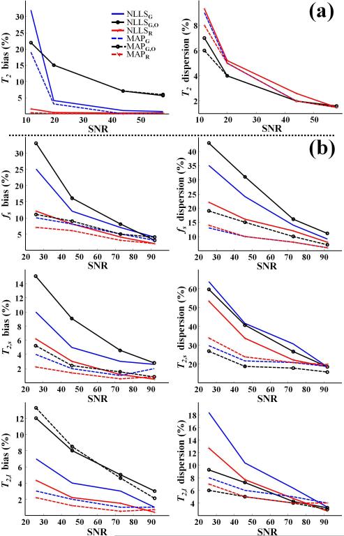
As for the MC simulations, results of the phantom measurements were obtained after removal of VEO. Figure 6 shows the relative bias and dispersion, as a function of SNR, in parameter estimates determined from phantom measurements using single-phantom monoexponential (Fig 6a) and dual-phantom biexponential (Fig. 6b) data. At high SNR, all methods demonstrated low bias and dispersion. For the monoexponential case, at low to moderate SNR, the bias was substantially lower with NLLSR and MAPR than it was using the other methods for the estimation of T2 (Fig. 6a). The dispersion in the estimation of T2 was comparable among all methods. Similarly, for the biexponential analysis, bias in the estimates of T2,s and T2,l was minimized through use of NLLSR and MAPR (Fig. 6b). For fs, MAPR was found to demonstrate the least bias, although all of the Bayesian-based methods performed well with the exception of MAPG,O in the estimation of T2,l. This is likely attributable to the limited echo acquisition window, resulting in incomplete sampling of the decay of the T2,l component. This effect is also seen in the poor performance of NLLSG,O. In addition, the dispersion in estimates of all derived parameters obtained using the NLLS-based methods was substantially greater as compared to Bayesian-based estimates.
Fig. 6.
Phantom study results showing relative bias and dispersion in parameter estimates as a function of SNR using the fitting methods NLLSG, NLLSG,O, NLLSR, MAPG, MAPG,O and MAPR. (a) Results for T2, assuming the monoexponential signal model with T2 = 58 ms as the underlying parameter value. (b) Results for fs, T2,s and T2,l assuming the biexponential signal model with fs = 0.33, T2,s = 14 ms and T2,l = 112 ms as underlying parameter values. Overall, accuracy and precision were substantially improved through use of Rician noise model and Bayesian analysis; see text for detailed discussion.
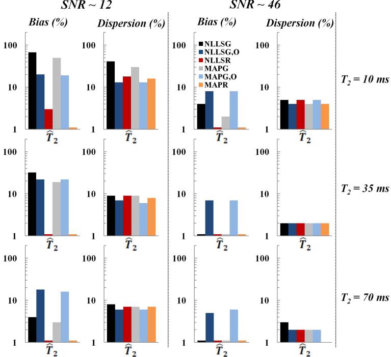
The effect of the underlying parameters T2, fs, T2,sand T2,l on the relative bias and dispersion in parameter estimates is summarized in Figs. 7-8. As shown, bias resulting from NLLSR and MAPR was the lowest, while dispersion using Bayesian-based methods was overall lower than using NLLS-based methods. In general, both bias and dispersion decreased with increasing T2 (Fig. 7). For the biexponential case, bias and dispersion both increase with a decreasing ratio T2,l/T2,s and with an increasing disparity between component sizes (Fig. 8).
Fig. 7.
Relative bias and dispersion obtained from phantom measurements for the estimation of T2, with a monoexponential signal model, for SNR of ~ 12 (left column) and ~ 46 (middle column), using NLLSG, NLLSG,O, NLLSR, MAPG, MAPG,O and MAPR analysis methods for three different input T2 values (right column). Improvements in accuracy and precision are seen through use of Rician noise model and Bayesian analysis, as discussed in the text.
In vivo Study
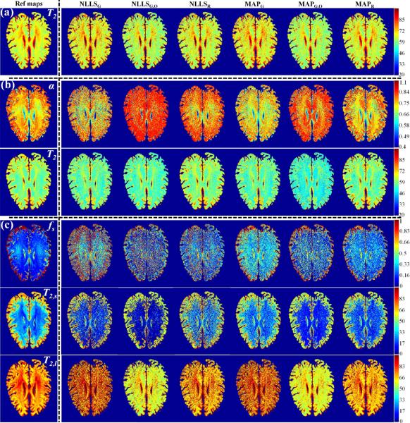
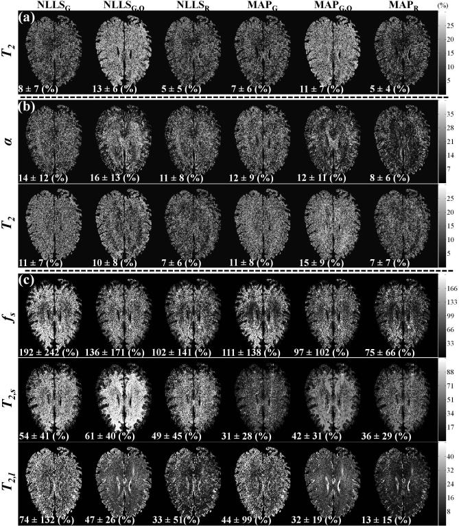
Figure 9 shows parameter maps derived from high SNR (~ 200) data (left hand column) using the six investigated methods, and corresponding parameter maps obtained at moderate SNR (~ 50), for monoexponential (Fig. 9a), stretched exponential (Fig. 9b) and biexponential (Fig. 9c) signal models. Figure 9 shows substantial random variation of estimated values in several image regions. To examine this in more detail, relative error maps, calculated as described in the Methods and describing the deviation of estimated parameter values from those obtained from the high SNR fiducial images, were created (Fig. 10). The mean and standard deviation of the relative errors are reported at the bottom of each error map. At the moderate SNR, all methods performed well for the estimation of T2 in monoexponential decay, although MAPR and NLLSR were the best. These two methods also showed the best performance for the estimation of T2 and α in the stretched exponential signal model. For biexponential analysis, the SNR was insufficient to provide a high-quality estimate of fs using any of the analysis approaches, although MAPR performed the best. T2,s and T2,l were estimated more accurately, although only T2,l could be estimated to within ~ 15%, as achieved by MAPR.
Fig. 9.
Reference parameter maps obtained at high SNR (~ 200) using the MAPR method (left column) and parameter maps obtained at moderate SNR (~ 50) using the fitting methods NLLSG, NLLSG,O, NLLSR, MAPG, MAPG,O and MAPR (columns from left to right). (a) T2 maps assuming the monoexponential signal model. (b) T2 and α maps assuming the stretched exponential signal model. (c) fs, T2,s and T2,l maps assuming the biexponential signal model. Greater consistency is achieved through use of Rician noise model and Bayesian analysis; see text for detailed discussion.
Fig. 10.
Relative error maps indicating the deviation of the parameter maps obtained at modest SNR (~ 50), shown in columns 2-7 of Fig. 9, from the high SNR fiducial map shown in column 1 of Fig. 9. The columns show the results obtained through use of NLLSG, NLLSG,O, NLLSR, MAPG, MAPG,O and MAPR for (a) the monoexponential signal model, (b) the stretched exponential signal model, and (c) the biexponential signal model. The mean and standard deviation of the relative error is given below each error map. Clear improvements are seen through use of Rician noise model and Bayesian analysis, as discussed in detail in the text.
DISCUSSION
Parameter Estimation Methods
Bayesian Probability vs NLLS Approaches
The elegant work of Neil and Bretthorst (17) evaluated estimates of diffusion parameters for a two-compartment model at two values of SNR, using both simulations and spectroscopic NMR data exhibiting Gaussian noise. Substantial advantages were found for Bayesian analysis as compared to NLLS in terms of both accuracy and precision. Our work builds on this and extends it in several ways, using simulations, and phantom and human brain imaging experiments. First, we evaluate three distinct and widely-used signal models for transverse decay, the monoexponential, stretched exponential and biexponential. In addition, for each of these models, we evaluate the performance of three approaches to incorporating noise, namely, the assumption of Gaussian noise, the assumption of Gaussian noise that asymptotes to a non-zero value, and the assumption of Rician noise, as is most appropriate for magnitude MR images. Further, we evaluated the accuracy and precision with which parameters of interest can be estimated for wide ranges of SNR and underlying parameters.
Overall, we found improved accuracy and precision using the Bayesian-based methods as compared to the NLLS-based methods (Figs. 2-8). This may be attributable to the fact that in Bayesian analysis, a given parameter is estimated independently of the others through marginalization, serving to reduce interdependence of parameter estimates by integrating over all values of the marginal parameters. This is in contrast to NLLS where unknown parameter estimates are highly correlated through the use of simultaneous estimation. This correlation has been previously demonstrated through Cramer-Rao lower bound calculations, MC simulations, and phantom measurements (8, 15-16). In addition, the NLLS algorithm may fail to find global minima due to the presence of local minima. Although such local minima are absent for the monoexponential, they are present for the bi- and stretched-exponential cases. This problem becomes more acute with the flattening of the surface of the least squares residuals seen with increasing model complexity (Supporting Figure S1). In fact, the performance of the Bayesian and NLLS methods were very similar for the monoexponential analysis, with the small differences being potentially attributable to the marginalization over A0.
Finally, we found that in spite of its additional model complexity, potentially leading to substantial analytic difficulties, the performance of MAPR provides notable improvement in accuracy and precision compared to NLLSR.
Rician vs Gaussian noise models
Our analyses show substantial improvements in accuracy and precision when Rician noise model is incorporated into the analysis of magnitude imaging data, with estimates performed through either NLLS or Bayesian analyses. Similar results have been previously reported for the estimation of T1, T2 and T2* using NLLS (12-13, 15), and for the estimation of T2 using Bayesian analysis (21).
It is common practice to assume Gaussian-distributed noise in conventional magnitude MR images with high SNR (42, 63-66). Our results (Figs. 2-8) serve to validate this and demonstrate that high-quality parameter estimates may be obtained with the Gaussian approximation. However, we found that with more modest SNR, there is a substantial loss of performance. Attempting to compensate for the asymptotic positivity of the noise by using Gaussian noise with offset model was found to be of benefit when fitting data with small T2, for which the signal is dominated by noise in the later echoes.
Unknown vs estimated noise parameters
All calculations were performed assuming known values for σ, σ2 and, ε, such as would be based on separate measurements in order to reduce the dimensionality of parameter space. As expected, MC simulations (data not shown) indicate that this strategy resulted in increased accuracy, presumably through reducing the number of local minima and the interdependence of parameter estimates. A modest increase in precision was also found. In addition, computational times were considerably reduced, particularly for the Bayesian-based methods since marginalization over σ was not needed.
The quality of parameter estimates of course depends upon the quality of the estimates of . Simulation analysis (Supporting Table S1) indicates that, as expected, moderate errors in the estimation of noise parameters, such as would be the case for estimation from large background regions of the image, have a negligible impact on parameter estimates. This was found to be the case for all fitting methods and for all three signal models. Clearly, the presence of non-random artifacts such as streaking or ghosting requires more sophisticated estimates of noise (67-68). In any event, in actual application, the strategy of independent noise estimation is to be preferred over incorporation of yet another parameter into the Bayesian or NLLS analysis.
Results of NLLS and Bayesian Probability Approaches
Performance of the NLLS-based methods
All three NLLS-based methods were found to be sensitive to initial estimates, highlighting the necessity of establishing a reproducible algorithm for selection of these estimates, especially in the low SNR regime. In contrast, at high SNR, convergence to global minima was attained even for relatively poor initial estimates (data not shown). However, in spite using true parameter values as starting points, we found a loss of performance as the total number of unknown parameters increased, such as in comparing the monoexponential to the biexponential. This is likely attributable to the increase in the number of local minima and to the flattening of the surface of least squares residuals as the number of parameters increases (Supporting Figure S1).
In some cases, we found that NLLSR compared favorably to MAPR. However, our approach implemented an unrealistically favorable NLLSR analysis by providing true values as starting parameters, while in actual experiments these values are of course not known. It is well-known that inaccurate initial guesses render the NLLS algorithm highly susceptible to finding local rather than global minima (69), so that this procedure in effect penalizes the Bayesian analysis as compared to NLLS.
Performance of the Bayesian-based methods
One drawback of the Bayesian approaches is the computational time required to compute the integrals needed for the marginalization. In our direct implementation, computational time increased considerably with increasing dimensionality of the parameter space. To address this, the Markov Chain Monte Carlo method can be used so that the posterior distribution can be sampled, rather than directly computed (20, 70).
Numerical Simulations, Phantom and In vivo Studies
Our simulation results show that in the limit of high SNR, all six investigated methods yielded results that were accurate and precise. However, large differences in performance were seen at low to moderate SNR. Overall, MAPR performed the best of all methods, although NLLSR provided comparable results in many cases. As an example, the accuracy and precision of the estimate of the fraction of the rapidly decaying component, fs, in the biexponential model were greatly improved using MAPR as compared to the other methods, including NLLSR. This is of particular importance, since fs has been proposed as a biomarker of pathology in several biological tissues, including cartilage (1-2, 38-39), bone (51) and brain (3-7, 40).
Our in vivo brain study indicates that, as expected, any of the six methods works well at high SNR. However, MAPR provides the most robust parameter estimates, especially in the low SNR regime. This can be seen visually from the parameter maps (Fig. 9) and from the error maps (Fig. 10). In contrast to MC simulations and phantom experiments, for the in vivo analyses there was no underlying correct model for comparison, and both monoexponential and biexponential models have been used in the analyses of transverse relaxation data from brain. In diffusion studies of brain, mono-, bi- and stretched-exponentials have all been applied (14, 43, 46, 71-73).
We found that in general, methods incorporating Rician noise performed better than those using Gaussian noise, regardless of the signal model. This is in agreement with previous work on cartilage for monoexponential T2 (12) and biexponential T2* (15) measurements. Our results also indicate that Bayesian-based methods exhibit higher precision than NLLS-based methods.
Our MC simulations, and phantom and in vivo experiments, all highlight the importance of considering the correct form of the noise distribution for magnitude MR images. We have used the Rician distribution, as is appropriate for single-coil signal reception. However, multiple receiver coils are widely used to increase speed or SNR. If uncorrelated, equally distributed and stationary noise is assumed, the noise distribution in the resulting magnitude images is described by a non-central χ-distributions
where R denotes the number of channels (55, 74). The corresponding likelihood function is given by
This expression can be incorporated into a Bayesian approach for parameter estimation in a fashion analogous to the above. This can be compared to an NLLS minimization using the first moment of Pχ(Sn | A(θ;TEn),σ,R) as the expectation value of the acquired data
(75-78), where 1F1 is a confluent hypergeometric function.
Our results indicate that in general, Bayesian analysis provides more reliable estimates of transverse decay parameters than does NLLS when the underlying signal model is known. In realistic experiments, the correct signal model may be unknown. We believe that previous results (17, 20, 79) and the results presented here provide strong motivation for investigations of model selection using Bayesian probability theory.
Supplementary Material
ACKNOWLEDGEMENTS
We gratefully acknowledge the anonymous reviewers for their helpful comments. This work was supported by the Intramural Research Program of the NIH, National Institute on Aging.
APPENDIX
We define details of the marginalization used in Bayesian parameter estimation. To obtain the estimated parameter, , (Eqs. A1-A6), the corresponding posterior probability, P(θi | S,σ), was computed for a grid of parameter values, θi. The MAP estimate, , corresponds to the value for which P(θi | S,σ) attains the maximum of the computed values (17, 20-21, 37). Integrals were performed numerically using the integral, integral2 and integral3 commands in Matlab for mono-, stretched-, and biexponential signal models, respectively. The integration limits were chosen such that the contribution of the relevant likelihood function to the integral outside these limits was negligible.
Bayesian inference requires assignment of a prior probability based on pre-existing knowledge (80). This choice becomes of particular importance when the likelihood function is not the dominant term in the posterior probability such as is often the case when only a limited number of measurements are available (37). In the present work, the number of measurements was much greater than the number of derived parameters, so that results are largely independent of reasonable selections of prior probabilities (data not shown). We assumed a formally improper uniform prior in all cases; that is, the P(θ) term in Eq. 7 was taken as unity. With limited data, the selection of the prior is more critical (37).
Likelihood functions for Bayesian-based methods
Each Bayesian-based method is defined by its likelihood function, L(S|θ,σ) and a uniform prior. For MAPR , L(S|θ,σ) = LRice(S|θ,σ) (Eq. 3), for MAPG , L(S|θ,σ) = LGauss(S|θ,σ) (Eq. 6), and for MAPG,O, L(S|θ,σ) = LGauss(S|θ,σ) with A(θ;TEn) in Eq. 6 replaced by A(θ;TEn) + ε.
Marginalization Integrals for Signal Models
Monoexponential Signal Model
The estimate of T2 was obtained according to
| [A.1] |
where A(θ;TEn) is given by Eq. 10.
Stretched Exponential Signal Model
Estimates of T2 and α were obtained according to
| [A.2] |
| [A.3] |
where A(θ;TEn) is given by Eq. 11.
Biexponential Signal Model
Estimates of fs, T2,s and T2,l were obtained according to
| [A.4] |
| [A.5] |
| [A.6] |
where A(θ;TEn) is given by Eq. 12.
REFERENCES
- 1.Reiter DA, Roque RA, Lin PC, Doty SB, Pleshko N, Spencer RG. Improved Specificity of Cartilage Matrix Evaluation using Multiexponential Transverse Relaxation Analysis Applied to Pathomimetically Degraded Cartilage. NMR Biomed. 2011;24:1286–1294. doi: 10.1002/nbm.1690. [DOI] [PMC free article] [PubMed] [Google Scholar]
- 2.Reiter DA, Lin PC, Fishbein KW, Spencer RG. Multicomponent T2 Relaxation Analysis in Cartilage. Magn Reson Med. 2009;61:803–809. doi: 10.1002/mrm.21926. [DOI] [PMC free article] [PubMed] [Google Scholar]
- 3.MacKay A, Laule C, Vavasour I, Bjarnason T, Kolind S, Mädler B. Insights into Brain Microstructure from the T2 Distribution. Magn Reson Imaging. 2006;24:515–525. doi: 10.1016/j.mri.2005.12.037. [DOI] [PubMed] [Google Scholar]
- 4.Webb S, Munro CA, Midha R, Stanisz GJ. Is Multicomponent T2 a good Measure of Myelin Content in Peripheral Nerve? Magn Reson Med. 2003;49:638–645. doi: 10.1002/mrm.10411. [DOI] [PubMed] [Google Scholar]
- 5.Kolind SH, Laule C, Vavasour IM, Li DK, Traboulsee AL, Mädler B, Moore GR, MacKay AL. Complementary Information from Multi-exponential T2 Relaxation and Diffusion Tensor Imaging Reveals Differences between Multiple Sclerosis Lesions. Neuroimage. 2008;40:77–85. doi: 10.1016/j.neuroimage.2007.11.033. [DOI] [PubMed] [Google Scholar]
- 6.Junyu Guo, Qing Ji, Wilburn E. Reddick. Multi-slice Myelin Water Imaging for Practical Clinical Applications at 3.0 T. Magn Reson Med. 2013;70:813–822. doi: 10.1002/mrm.24527. [DOI] [PMC free article] [PubMed] [Google Scholar]
- 7.Harkins KD, Valentine WM, Gochberg DF, Does MD. In vivo Multi-exponential T2, Magnetization Transfer and Quantitative Histology in a Rat Model of Intramyelinic Edema. Neuroimage Clin. 2013;2:810–817. doi: 10.1016/j.nicl.2013.06.007. [DOI] [PMC free article] [PubMed] [Google Scholar]
- 8.Celik H, Bouhrara M, Reiter DA, Fishbein KW, Spencer RG. Stabilization of the Inverse Laplace Transform of Multiexponential Decay through Introduction of a Second Dimension. J Magn Reson. 2013;236:134–139. doi: 10.1016/j.jmr.2013.07.008. [DOI] [PMC free article] [PubMed] [Google Scholar]
- 9.Day IJ. On the Inversion of Diffusion NMR Data: Tikhonov Regularization and Optimal Choice of the Regularization Parameter. J Magn Reson. 2011;211:178–185. doi: 10.1016/j.jmr.2011.05.014. [DOI] [PubMed] [Google Scholar]
- 10.Rice SO. Mathematical analysis of random noise. In: Wax N, editor. Selected papers on noise and stochastic processes. Dover Publications Inc.; New York, NY: 1954. pp. 133–194. [Google Scholar]
- 11.Bernstein MA, Thomasson DM, Perman WH. Improved Detectability in Low Signal-to-Noise Ratio Magnetic Resonance Images by Means of Phase-corrected Real Reconstruction. Med Phys. 1989;16:813–817. doi: 10.1118/1.596304. [DOI] [PubMed] [Google Scholar]
- 12.Raya JG, Dietrich O, Horng A, Weber J, Reiser MF, Glaser C. T2 Measurement in Articular Cartilage: Impact of the Fitting Method on Accuracy and Precision at Low SNR. Magn Reson Med. 2010;63:181–193. doi: 10.1002/mrm.22178. [DOI] [PubMed] [Google Scholar]
- 13.Karlsen OT, Verhagen R, Bovée WMMJ. Parameter Estimation From Rician-Distributed Data Sets Using a Maximum Likelihood Estimator: Application to T1 and Perfusion Measurements. Magn Reson Med. 1999;41:614–623. doi: 10.1002/(sici)1522-2594(199903)41:3<614::aid-mrm26>3.0.co;2-1. [DOI] [PubMed] [Google Scholar]
- 14.Kristoffersen A. Estimating Non-Gaussian Diffusion Model Parameters in the Presence of Physiological Noise and Rician Signal Bias. J Magn Reson Imaging. 2012;35:181–189. doi: 10.1002/jmri.22826. [DOI] [PubMed] [Google Scholar]
- 15.Bouhrara M, Reiter DA, Celik H, Bonny JM, Lukas V, Fishbein KW, Spencer GS. Incorporation of Rician Noise in the Analysis of Biexponential Transverse Relaxation in Cartilage using a Multiple Gradient Echo Sequence at 3 and 7 Tesla. Magn Reson Med. 2014 doi: 10.1002/mrm.25111. DOI: 10.1002/mrm.25111. [DOI] [PMC free article] [PubMed] [Google Scholar]
- 16.Anastasiou A, Hall LD. Optimization of T2 and M0 Measurements of Biexponential Systems. Magn Reson Imaging. 2004;22:67–80. doi: 10.1016/j.mri.2003.05.005. [DOI] [PubMed] [Google Scholar]
- 17.Neil JJ, Bretthorst GL. On the use of Bayesian Probability Theory for Analysis of Exponential Decay Data: an Example Taken from Intravoxel Incoherent Motion Experiments. Magn Reson Med. 1993;29:642–647. doi: 10.1002/mrm.1910290510. [DOI] [PubMed] [Google Scholar]
- 18.Orton MR, Collins DJ, Walker-Samuel S, d'Arcy JA, Hawkes DJ, Atkinson D, Leach MO. Bayesian Estimation of Pharmacokinetic Parameters for DCE-MRI with a Robust Treatment of Enhancement Onset Time. Phys Med Biol. 2007;52:2393–2408. doi: 10.1088/0031-9155/52/9/005. [DOI] [PubMed] [Google Scholar]
- 19.Transtrum MK, Machta BB, Sethna JP. Why are nonlinear fits to data so challenging? Phys Rev Lett. 2010;104:060201. doi: 10.1103/PhysRevLett.104.060201. [DOI] [PubMed] [Google Scholar]
- 20.Bretthorst GL, Hutton WC, Garbow JR, Ackerman JJH. Exponential Parameter Estimation (in NMR) Using Bayesian Probability Theory. Concepts in Magn Reson. 2005;27A:55–63. [Google Scholar]
- 21.Walker-Samuel S, Orton M, McPhail LD, Boult JK, Box G, Eccles SA, Robinson SP. Bayesian Estimation of Changes in Transverse Relaxation Rates. Magn Reson Med. 2010;64:914–921. doi: 10.1002/mrm.22478. [DOI] [PubMed] [Google Scholar]
- 22.Papoulis A. Probability, random variables and stochastic processes. second McGraw-Hill; Tokyo: 1984. [Google Scholar]
- 23.Sijbers J, den Dekker AJ, Verhoye M, Van Audekerke J, Van Dyck D. Estimation of Noise from Magnitude MR Images. Magn Reson Imaging. 1998;16:87–90. doi: 10.1016/s0730-725x(97)00199-9. [DOI] [PubMed] [Google Scholar]
- 24.Lehmann EL, Casella G. Theory of Point Estimation. second Springer-Verlag; New York. 1998. [Google Scholar]
- 25.Gudbjartsson H, Patz S. The Rician Distribution of Noisy MRI Data. Magn Reson Med. 1995;34:910–914. doi: 10.1002/mrm.1910340618. [DOI] [PMC free article] [PubMed] [Google Scholar]
- 26.Kroenke CD, Bretthorst GL, Inder TE, Neil JJ. Modeling Water Diffusion Anisotropy Within Fixed Newborn Primate Brain Using Bayesian Probability Theory. Magn Reson Med. 2006;55:187–197. doi: 10.1002/mrm.20728. [DOI] [PubMed] [Google Scholar]
- 27.Bretthorst GL. Lecture Notes in Statistics. Vol. 48. Springer-Verlag; New York: 1988. Bayesian Spectrum Analysis and Parameter Estimation. [Google Scholar]
- 28.Bretthorst GL. Bayesian Analysis I. Parameter Estimation Using Quadrature NMR Models. J Magn Reson. 1990;88:533–551. [Google Scholar]
- 29.Xing D, Gibbs SJ, Derbyshire JA, Fordham EJ, Carpenter TA, Hall LD. Bayesian Analysis for Quantitative NMR Flow and Diffusion Imaging. J Magn Reson. 1995;106:1–9. [Google Scholar]
- 30.Quirk JD, Sukstanskii AL, Bretthorst GL, Yablonskiy DA. Optimal Decay Rate Constant Estimates from Phased Array Data utilizing Joint Bayesian Analysis. J Magn Reson. 2009;198:49–56. doi: 10.1016/j.jmr.2009.01.001. [DOI] [PMC free article] [PubMed] [Google Scholar]
- 31.Üstündağ D, Cevri M. Recovering Sinusoids from Noisy Data using Bayesian Inference with Simulated Annealing. Math Comput Appli. 2011;16:382–391. [Google Scholar]
- 32.Payne SJ. A Bayesian Approach for the Estimation of Model Parameters from Noisy Data Sets. IEEE Signal Proc Letters. 2005;12:553–556. [Google Scholar]
- 33.Jbabdi S, Woolrich MW, Andersson JL, Behrens TE. A Bayesian Framework for Global Tractography. NeuroImage. 2007;37:116–129. doi: 10.1016/j.neuroimage.2007.04.039. [DOI] [PubMed] [Google Scholar]
- 34.Jbabdi S, Sotiropoulos SN, Savio AM, Graña M, Behrens TE. Model-based Analysis of Multishell Diffusion MR Data for Tractography: How to get over Fitting Problems. Magn Reson Med. 2012;68:1846–1855. doi: 10.1002/mrm.24204. [DOI] [PMC free article] [PubMed] [Google Scholar]
- 35.Bayes T. An Essay towards solving a Problem in the Doctrine of Chances. Philosophical Transactions of the Royal Society of London. 1763;53:370–418. [Google Scholar]
- 36.Laplace P. Mémoire sur la Probabilité des Causes par les Evènements. l'Académie Royale des Sciences. 1774;61:621–656. 359–378. English translation by S.M. Stigler in 1986 as "Memoir on the Probability of the Causes of Events" in Statistical Science. [Google Scholar]
- 37.Murphy KP. Machine Learning: a Probabilistic Perspective. The MIT Press; 2012. [Google Scholar]
- 38.Reiter DA, Roque RA, Lin PC, Irrechukwu O, Doty S, Longo DL, Pleshko N, Spencer RG. Mapping Proteoglycan-Bound Water in Cartilage: Improved Specificity of Matrix Assessment using Multiexponential Transverse Relaxation Analysis. Magn Reson Med. 2011;65:377–384. doi: 10.1002/mrm.22673. [DOI] [PMC free article] [PubMed] [Google Scholar]
- 39.Xia Y, Moody JB, Alhadlaq H. Orientational Dependence of T2 relaxation in Articular Cartilage: a Microscopic MRI (micro MRI) Study. Magn Reson in Med. 2002;48:460–469. doi: 10.1002/mrm.10216. [DOI] [PubMed] [Google Scholar]
- 40.Meyers SM, Laule C, Vavasour IM, Kolind SH, Mädler B, Tam R, Traboulsee AL, Lee J, Li DK, MacKay AL. Reproducibility of Myelin Water Fraction Analysis: a Comparison of Region of Interest and Voxel-based Analysis Methods. Magn Reson Imaging. 2009;27:1096–1103. doi: 10.1016/j.mri.2009.02.001. [DOI] [PubMed] [Google Scholar]
- 41.Deoni SC, Matthews L, Kolind SH. One Component? Two Components? Three? The Effect of Including a Nonexchanging "Free" Water Component in Multicomponent Driven Equilibrium Single Pulse Observation of T1 and T2. Magn Reson Med. 2013;70:147–154. doi: 10.1002/mrm.24429. [DOI] [PMC free article] [PubMed] [Google Scholar]
- 42.Whittall KP, MacKay AL, Li DK. Are Mono-exponential Fits to a Few Echoes Sufficient to Determine T2 Relaxation for In vivo Human Brain? Magn Reson Med. 1999;41:1255–1257. doi: 10.1002/(sici)1522-2594(199906)41:6<1255::aid-mrm23>3.0.co;2-i. [DOI] [PubMed] [Google Scholar]
- 43.Kristoffersen A. Optimized Quantification of Diffusional Non-Gaussianity in the Human Brain. J Magn Reson Imaging. 2013;38:1434–1444. doi: 10.1002/jmri.24102. [DOI] [PubMed] [Google Scholar]
- 44.Hall MG, Barrick TR. From Diffusion-Weighted MRI to Anomalous Diffusion Imaging. Magn Reson Med. 2008;59:447–455. doi: 10.1002/mrm.21453. [DOI] [PubMed] [Google Scholar]
- 45.Palombo M, Gabrielli A, De Santis S, Capuani S. The γ Parameter of the Stretched-exponential Model is Influenced by Internal Gradients: Validation in Phantoms. J Magn Reson. 2012;216:28–36. doi: 10.1016/j.jmr.2011.12.023. [DOI] [PubMed] [Google Scholar]
- 46.Ingo C, Magin RL, Colon-Perez L, Triplett W, Mareci TH. On random Walks and Entropy in Diffusion-weighted Magnetic Resonance Imaging Studies of Neural Tissue. Magn Reson Med. 2013;71:617–627. doi: 10.1002/mrm.24706. [DOI] [PMC free article] [PubMed] [Google Scholar]
- 47.Magin RL, Li W, Pilar Velasco M, Trujillo J, Reiter DA, Morgenstern A, Spencer RG. Anomalous NMR Relaxation in Cartilage Matrix Components and Native Cartilage: Fractional-order Models. J Magn Reson. 2011;210:184–191. doi: 10.1016/j.jmr.2011.03.006. [DOI] [PMC free article] [PubMed] [Google Scholar]
- 48.Lattanzio PJ, Marshall KW, Damyanovich AZ, Peemoeller H. Macromolecule and Water Magnetization Exchange Modeling in Articular Cartilage. Magn Reson Med. 2000;44:840–851. doi: 10.1002/1522-2594(200012)44:6<840::aid-mrm4>3.0.co;2-k. [DOI] [PubMed] [Google Scholar]
- 49.Ababneh Z, Beloeil H, Berde CB, Gambarota G, Maier SE, Mulkern RV. Biexponential Parameterization of Diffusion and T2 Relaxation Decay Curves in a Rat Muscle Edema Model: Decay Curve Components and Water Compartments. Magn Reson Med. 2005;54:524–531. doi: 10.1002/mrm.20610. [DOI] [PubMed] [Google Scholar]
- 50.Diaz E, Chung CB, Bae WC, Statum S, Znamirowski R, Bydder GM, Du J. Ultrashort Echo Time Spectroscopic Imaging (UTESI): an Efficient Method for Quantifying Bound and Free Water. NMR Biomed. 2012;25:161–168. doi: 10.1002/nbm.1728. [DOI] [PubMed] [Google Scholar]
- 51.Du J, Bydder GM. Qualitative and Quantitative Ultrashort-TE MRI of Cortical Bone. NMR Biomed. 2013;26:489–506. doi: 10.1002/nbm.2906. [DOI] [PMC free article] [PubMed] [Google Scholar]
- 52.He T, Gatehouse PD, Smith GC, Mohiaddin RH, Pennell DJ, Firmin DN. Myocardial T2* Measurements in Iron-overloaded Thalassemia: an In vivo Study to Investigate Optimal Methods of Quantification. Magn Reson Med. 2008;60:1082–1089. doi: 10.1002/mrm.21744. [DOI] [PMC free article] [PubMed] [Google Scholar]
- 53.Juras V, Apprich S, Zbýň S, Zak L, Deligianni X, Szomolanyi P, Bieri O, Trattnig S. Quantitative MRI Analysis of Menisci Using Biexponential T2* Fitting with a Variable Echo Time Sequence. Magn Reson Med. 2014;71:1015–1023. doi: 10.1002/mrm.24760. [DOI] [PMC free article] [PubMed] [Google Scholar]
- 54.Ghugre NR, Enriquez CM, Coates TD, Nelson MD, Wood JC. Improved R2* Measurements in Myocardial Iron Overload. J Magn Reson Imaging. 2006;23:9–16. doi: 10.1002/jmri.20467. [DOI] [PMC free article] [PubMed] [Google Scholar]
- 55.Edelstein WA, Bottomley PA, Pfeifer LM. A Signal-to-Noise Calibration Procedure for NMR Imaging Systems. Med Phys. 1984;11:180–185. doi: 10.1118/1.595484. [DOI] [PubMed] [Google Scholar]
- 56.Constantinides CD, Atalar E, McVeigh ER. Signal-to-Noise Measurements in Magnitude Images from NMR Phased Arrays. Magn Reson Med. 1997;38:852–857. doi: 10.1002/mrm.1910380524. [DOI] [PMC free article] [PubMed] [Google Scholar]
- 57.Aja-Fernández S, Alberola-López C, Westin CF. Noise and Signal Estimation in Magnitude MRI and Rician Distributed Images: A LMMSE Approach. IEEE Trans Image Process. 2008;17:1383–1898. doi: 10.1109/TIP.2008.925382. [DOI] [PubMed] [Google Scholar]
- 58.Sijbers J, den Dekker AJ. Maximum Likelihood Estimation of Signal Amplitude and Noise Variance From MR Data. Magn Reson Med. 2004;51:586–594. doi: 10.1002/mrm.10728. [DOI] [PubMed] [Google Scholar]
- 59.Hoaglin D, Mosteller F, Tukey J. Understanding Robust and Exploratory Data Analysis. John Wiley & Sons; New York: 1983. [Google Scholar]
- 60.McGibney G, Smith MR. An Unbiased Signal-to-Noise Ratio Measure for Magnetic Resonance Imaging. Med Phys. 1993;20:1077–1078. doi: 10.1118/1.597004. [DOI] [PubMed] [Google Scholar]
- 61.Carr HY, Purcell EM. Effects of Diffusion on Free Precession in Nuclear Magnetic Resonance Experiments. Phys Rev. 1954;94:630–637. [Google Scholar]
- 62.Meiboom S, Gill D. Modified Spin-echo Method for Measuring Nuclear Relaxation Times. Rev Sci Intrum. 1958;29:688–691. [Google Scholar]
- 63.Bonny JM, Zanca M, Boire JY, Veyre A. T2 Maximum Likelihood Estimation from Multiple Spin-echo Magnitude Images. Magn Reson Med. 1996;36:287–296. doi: 10.1002/mrm.1910360216. [DOI] [PubMed] [Google Scholar]
- 64.Shrager RI, Weiss GH, Spencer RG. Optimal Sampling Strategies for T2 Measurements: Monoexponential and Biexponential Systems. NMR Biomed. 1998;11:297–305. doi: 10.1002/(sici)1099-1492(199810)11:6<297::aid-nbm531>3.0.co;2-a. [DOI] [PubMed] [Google Scholar]
- 65.Jones DK, Basser PJ. "Squashing Peanuts and Smashing Pumpkins": How Noise Distorts Diffusion-weighted MR Data. Magn Reson Med. 2004;52:979–993. doi: 10.1002/mrm.20283. [DOI] [PubMed] [Google Scholar]
- 66.Jones JA, Hodgkinson P, Barker AL, Hore PJ. Optimal Sampling Strategies for the Measurement of spin-spin Relaxation Times. J Magn Reson. 1996;113:25–34. [Google Scholar]
- 67.Coupé P, Manjón JV, Gedamu E, Arnold D, Robles M, Collins DL. Robust Rician Noise Estimation for MR Images. Med Image Anal. 2010;14:483–493. doi: 10.1016/j.media.2010.03.001. [DOI] [PubMed] [Google Scholar]
- 68.Rajan J, Poot D, Juntu J, Sijbers J. Segmentation Based Noise Variance Estimation from Background MRI Data. Proceedings of the 7th International Conference on Image Analysis and Recognition; Springer-Verlag. 2010. pp. 62–70. [Google Scholar]
- 69.Press WH, Teukolsky SA, Vetterling WT, Flannery BP. The Art of Scientific Computing. Cambridge University Press; Cambridge, UK: 1992. Numerical recipes in C. [Google Scholar]
- 70.Metropolis N, Ulam S. The Monte Carlo method. J Amer Statist Assoc. 1949;44:335–341. doi: 10.1080/01621459.1949.10483310. [DOI] [PubMed] [Google Scholar]
- 71.Bennett KM, Schmainda KM, Bennett RT, Rowe DB, Lu H, Hyde JS. Characterization of Continuously Distributed Cortical Water Diffusion Rates with a Stretched-exponential Model. Magn Reson Med. 2003;50:727–734. doi: 10.1002/mrm.10581. [DOI] [PubMed] [Google Scholar]
- 72.Grinberg F, Farrher E, Ciobanu L, Geffroy F, Le Bihan D, Shah NJ. Non-Gaussian Diffusion Imaging for Enhanced Contrast of Brain Tissue Affected by Ischemic Stroke. PloS One. 2014;27:e89225. doi: 10.1371/journal.pone.0089225. 9(2) [DOI] [PMC free article] [PubMed] [Google Scholar]
- 73.Mulkern RV, Haker SJ, Maier SE. On High b Diffusion Imaging in the Human Brain: Ruminations and Experimental Insights. Magn Reson Med. 2009;27:1151–1162. doi: 10.1016/j.mri.2009.05.003. [DOI] [PMC free article] [PubMed] [Google Scholar]
- 74.Miller KS. Multidimensional Gaussian Distributions. John Wiley and Sons Inc.; New York: 1964. pp. 26–42. [Google Scholar]
- 75.Koay CG, Basser PJ. Analytically Exact Correction Scheme for Signal Extraction from Noisy Magnitude MR Signals. J Magn Reson. 2006;179:317–322. doi: 10.1016/j.jmr.2006.01.016. [DOI] [PubMed] [Google Scholar]
- 76.Wang C, He T, Liu X, Zhong S, Chen W, Feng Y. Rapid Look-up Table Method for Noise-corrected Curve Fitting in the R2* Mapping of Iron Loaded Liver. Magn Reson Med. 2014 doi: 10.1002/mrm.25184. DOI: 10.1002/mrm.25184. [DOI] [PubMed] [Google Scholar]
- 77.Feng Y, He T, Gatehouse PD, Li X, Harith Alam M, Pennell DJ, Chen W, Firmin DN. Improved MRI R2* Relaxometry of Iron-loaded Liver with Noise Correction. Magn Reson Med. 2013;70:1765–1774. doi: 10.1002/mrm.24607. [DOI] [PubMed] [Google Scholar]
- 78.Hardy PA, Andersen AH. Calculating T2 in Images from a Phased Array Receiver. Magn Reson Med. 2009;61:962–969. doi: 10.1002/mrm.21904. [DOI] [PMC free article] [PubMed] [Google Scholar]
- 79.Bretthorst GL, Hutton WC, Garbow JR, Ackerman JJH. Exponential Model Selection (in NMR) using Bayesian Probability Theory. Concepts Magn Reson. 2005;27A:64–72. [Google Scholar]
- 80.Jaynes ET. Prior Probabilities. IEEE Trans Syst Sci Cybern. 1968;4:227–241. [Google Scholar]
Associated Data
This section collects any data citations, data availability statements, or supplementary materials included in this article.


