Comparative Evaluation of Registration Algorithms in Different Brain Databases With Varying Difficulty: Results and Insights

Abstract

Evaluating various algorithms for the inter-subject registration of brain magnetic resonance images (MRI) is a necessary topic receiving growing attention. Existing studies evaluated image registration algorithms in specific tasks or using specific databases (e.g., only for skull-stripped images, only for single-site images, etc.). Consequently, the choice of registration algorithms seems task- and usage/parameter-dependent. Nevertheless, recent large-scale, often multi-institutional imaging-related studies create the need and raise the question whether some registration algorithms can 1) generally apply to various tasks/databases posing various challenges; 2) perform consistently well, and while doing so, 3) require minimal or ideally no parameter tuning. In seeking answers to this question, we evaluated 12 general-purpose registration algorithms, for their generality, accuracy and robustness. We fixed their parameters at values suggested by algorithm developers as reported in the literature. We tested them in 7 databases/tasks, which present one or more of 4 commonly-encountered challenges: 1) inter-subject anatomical variability in skull-stripped images; 2) intensity homogeneity, noise and large structural differences in raw images; 3) imaging protocol and field-of-view (FOV) differences in multi-site data; and 4) missing correspondences in pathology-bearing images. Totally 7,562 registrations were performed. Registration accuracies were measured by (multi-)expert-annotated landmarks or regions of interest (ROIs). To ensure reproducibility, we used public software tools, public databases (whenever possible), and we fully disclose the parameter settings. We show evaluation results, and discuss the performances in light of algorithms’ similarity metrics, transformation models and optimization strategies. We also discuss future directions for the algorithm development and evaluations.

I. Introduction

Image registration is a process of transforming different images into the same spatial coordinate system, so that after registration, the same spatial locations in different images represent the same anatomical structures. Image registration, especially deformable image registration, is a fundamental problem in medical image computing. It is usually an indispensable component in many analytic studies, including studies aiming to understand population trends of imaging phenotypes, to measure longitudinal changes, to fuse multi-modality information, to guide computerized interventions, to capture structure-function correlations, and many others (two recent comprehensive surveys can be found in [1], [2]; various other surveys can be found in [3]–[9]).

The past two decades have witnessed the development of many deformable registration algorithms. A comprehensive evaluation of different registration methods has thus become a research topic of interest. It is the basis for users to choose the most suitable methods for the problems at hand, and for algorithm developers to be better informed theoretically. A comprehensive evaluation is a fairly complicated problem, though. It oftentimes requires public databases, expert-labeling of ground truth regions/landmarks, a comprehensive evaluation protocol, careful tunings of parameters, considerable computational resources, and a proper choice of data to reflect certain registration challenges or to meet certain (pre-)clinical needs.

A. Literature on Evaluation of Algorithms in Brain MRI Registration

West et al. [10] evaluated 3 registration methods for multi-modal registration of the same subject undergoing neurosurgery, where the accuracy was measured on the fiducial markers. Hellier et al. [11] evaluated six methods (ANIMAL, Demons, SICLE, Mutual Information, Piecewise Affine, and the authors’ own method) in a database containing brain MRI from 18 healthy subjects; they measured registration accuracy on expert-defined cortical regions. Yanovsky et al. [12] evaluated three methods (fluid and two variations of the authors’ own methods, namely symmetric and asymmetric unbiased methods), in mapping brains during longitudinal scans for the detection of atrophy. They used 20 subjects from the ADNI database, and all images were preprocessed to exclude skull and dura. Yassa et al. [13] evaluated three methods (DARTEL, LDDMM, and Diffeomorphic Demons) in inter-subject registration of images especially at the medial temporal lobe, which is a crucial region for the study of memory. Christensen et al. introduced the NIREP project [14], [15], which in the first phase contains 16 publicly-available MR images, each having 32 expert-defined regions of interests (ROIs). They also defined a comprehensive set of evaluation criteria (including intensity-based variations, region-based overlaps, and transitivity errors). Based on these criteria they evaluated six methods (rigid, affine, AIR, Demons, SICLE, SLE) in [16]. Klein et al. in [17] evaluated 14 publicly-available registration tools for inter-subject registration of brain MR images. Four databases, each containing images of multiple subjects, were used. While it evaluated perhaps the largest number of registration tools so far, [17] only focused on skull-stripped, high quality, and single-site images from healthy subjects. To evaluate registration methods under more challenges, Klein et al. in another study [18] included both skull-stripped and raw images. Here, raw images refer to those acquired directly from scanner, prior to any image processing steps.

B. Need for a More Comprehensive Evaluation Study

While all the aforementioned studies provided insightful and informative evaluations, each study only tested registration methods in a specific task. For instance, for healthy subjects only (e.g., [11], [13], [16], [17]), for multi-modal fusion for pathological subjects only (e.g., [10]), for skull-stripped images only (e.g., [12], [13], [17]), for raw images only (e.g., [10], [11], [19]), for skull-stripped and raw images only (e.g., [18]), for single-site data only (e.g., [10], [11], [13], [16], [17]), and for multi-site data only (e.g., [12]). In addition, different evaluation studies included different registration methods for evaluation. Moreover, they used different parameter settings for a same registration method. As a result, the choice of registration algorithms seemed to be task- and database-dependent, and was sensitive to parameter settings.

Nevertheless, many of today’s large-scale, pre-clinical and imaging-related studies present a wide variety of challenges—they may contain normal-appearing and/or pathology-bearing images; they may contain skull-stripped and/or raw images; and they may contain images acquired from single- and/or multi-institutions. Facing all these possible challenges, there is an increasing need for registration algorithms that are publicly-available, that can widely apply to various tasks/databases, that can perform relatively accurately and robustly, that can be easily used by people with varying expertise in image registration, and that are without much need for parameter tunings.

While automatically and effectively tuning parameters for specific database/tasks is an important and active area of research (e.g., [20]–[24]), having registration algorithms that can be widely applicable to many tasks/databases is a very desirable property. This need stems not only from the size of studies, but also from the rapidly increasing number of studies undertaken in, for instance, translational neuroscience. Due to the lack of ground truth, tuning parameters is a difficult task even for technical experts. Moreover, when images are acquired and processed in multiple collaborative institutions, having registration algorithms that perform robustly and consistently well with a fixed set of parameters becomes almost entirely necessary.

C. Overview and Contributions of Our Evaluation Study

Towards meeting this need, this paper evaluates 12 publicly-available and general-purpose registration algorithms, including an attribute-based algorithm and 11 other intensity-based algorithms. Our work built upon and significantly expands previous evaluation studies of the similar nature in many aspects.

1. Our work evaluated registration methods under various tasks and databases presenting a wide variety of challenges, rather than in a specific task containing specific challenges. We identified four typical challenges in inter-subject registration of brain MRI (as will be described in Section II). We chose seven databases, each containing images of multiple subjects, to represent some or all of those challenges. This helped reveal whether a registration method could be generally applicable and robust with regard to various challenges.

2. To reflect the robustness of registration algorithms especially in multiple large-scale translational studies involving various tasks/databases, we fixed the parameters for each registration method throughout this paper (i.e., task-independent parameter settings). Particularly, in all tasks/databases in this paper, we used the parameters as the ones reported in [17] whenever applicable. Using such parameter settings was because that the parameters had been “optimized” by authors/developers of each specific algorithm for the registration of skull-stripped, preprocessed and normal-appearing brain MR images, which is a typical task in the inter-subject registration [17]. We realize that this set of parameters might not be optimal for other databases/tasks (e.g., those containing raw images, pathology-bearing images, or multi-site images). However, having a fixed set of parameters is perhaps how those registration algorithms would be used or first tried in daily imaging-related translational studies, where heavy parameter tunings are not only tedious, but also less practical or reproducible. From another perspective, it would be preferable if some registration algorithms could apply widely and could perform consistently well in various tasks/databases giving a fixed set of parameters.

To maintain reproducibility of our study, we used public databases wherever possible (six out of seven databases used in this paper are public); we included registration algorithms/tools that are publicly available; and we will fully disclose the exact parameter settings in Appendix B.

The rest of the paper is organized as follows. In Section II, we identify four typical challenges in the inter-subject registration of brain MR images. In Section III, we present the protocol to evaluate the accuracies of registration algorithms. In Section IV, we show the evaluation results. Finally, we discuss and conclude this paper in Section V.

II. Typical Challenges in Inter-Subject Brain MRI Registration

Brain images from different subjects may present one or more of the following challenges to registration.

Challenge 1: Inter-Subject Anatomical Variability

Subjects may vary structurally (Fig. 1 shows some examples). Inter-subject variability is a common challenge in many registration tasks investigating neuro-development, neuro-degeneration, or neuro-oncology. It is the main challenge against which registration methods were evaluated in the literature [13], [15]–[17].

Fig. 1.

Four randomly-chosen subjects in the NIREP database (the top two rows) and four randomly-chosen subjects in the LONI-LPBA40 database (the bottom two rows). For each subject, both the intensity image and the expert-annotated ROI image are shown. Different colors represent different ROIs in each database. These two databases were used to evaluate how registration methods perform facing challenges arising from the inter-subject variability (Challenge 1).

Challenge 2: Intensity Inhomogeneity, Noise and Structural Difference in Raw Images

In addition to inter-subject anatomical variability, images may suffer from intensity inhomogeneity (due to bias field), background noise, and low contrast. With skulls, ears, neck structures present in the raw images, subjects may also present larger deformations in those nonbrain structures compared to cortical structures (see Fig. 2 for example). Registration of raw images is necessary when 1) skull stripping is erroneous, so one has to work with the with-skull raw images; or 2) when registration itself is part of the skull-stripping step (e.g., in multi-atlas-based skull stripping approaches [19], [25]).

Fig. 2.

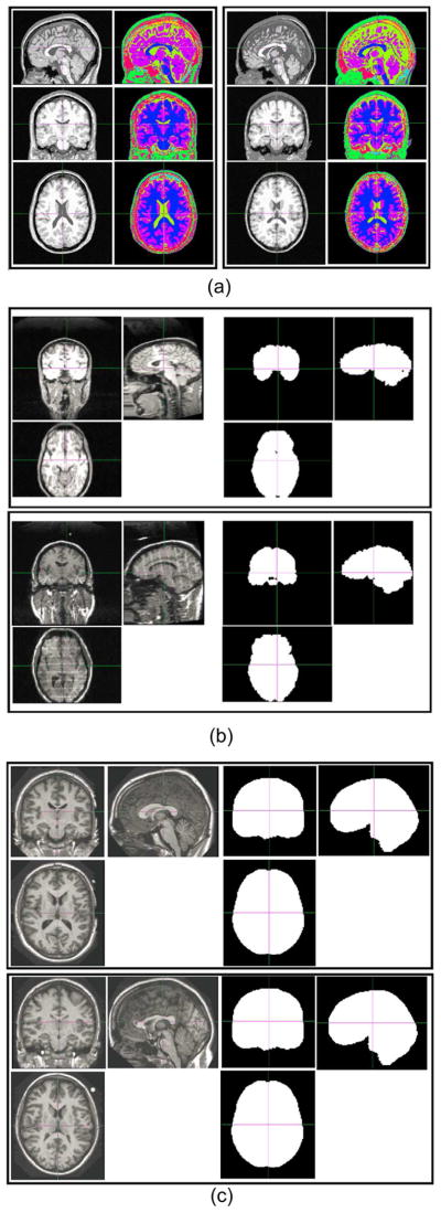
Images and annotations of two randomly chosen subjects from each of the three databases we used to represent Challenge 2 (intensity inhomogeneity, noise and structural differences in raw brain images). (a) From the BrainWeb database. (b) From the IBSR database. (c) From the OASIS database.

Challenge 3: Protocol and FOV Differences in Multi-site Databases

Many of today’s large-scale translational imaging-related studies involve brain MR images acquired from multiple institutions. Since MR scanners, imaging protocols, and FOVs may vary from institution to institution, the acquired images may vary greatly. Especially when the FOV is different, which is not uncommon in multi-site databases, some images may contain structures that do not show up in other images (see Fig. 3 for an example). One can rely on experts to interactively crop images, so that images from various institutions cover roughly the same FOV. However, the manual cropping is labor-intensive, subject to intra-/inter-rater variability, and may become intractable for today’s large-scale studies. Seeking a registration method that is relatively more robust to imaging protocol and FOV differences is therefore of interest.

Fig. 3.

Three-plane view of the intensity images and annotation images from three randomly-chosen subjects in the ADNI database. White color in the annotation images denotes the brain masks, and red denotes hippocampus masks. Blue contours in panel (a) point to the region that exists in one image, but does not exist in other images, due to the FOV differences in multiple imaging institutions. The ADNI database was used to represent Challenge 3 (on top of Challenges 1, 2). (a) A normal control (NC) subject. (b) A mild-cognitive-impairment (MCI) subject. (c) An Alzheimer’s Disease (AD) subject.

Challenge 4: Pathology-induced Missing Correspondences in Pathology-Bearing Images

Spatially normalizing a number of pathology-bearing images into a normal-appearing template space offers opportunities to understand the common spatial patterns of diseases. Pathologies present in the patients’ images, but not in the normal-appearing template. This poses the so-called missing correspondence problem (see Fig. 4 for example). An ideal registration approach should accurately align the normal regions (which do have correspondences across images), and relax the deformation in the pathology-affected regions, where no correspondences can be found [26], [27]. Literature has suggested to either mask out the pathological regions from the registration process (i.e., the cost-function-masking approach [27]), or, to simulate a pathological region in the normal-appearing template (i.e., the pathology-seeding approach [28]–[34]). However, both approaches require a careful segmentation of the pathological regions, which in itself is not an easy or affordable task, especially in large-scale studies. It is ideal if a general-purpose registration algorithm, segmentation-free in itself, can perform well in pathological-to-normal subject registration. That is, without prior knowledge of the presence or the location of the pathologies, nor any partition of the pathological versus normal regions, it is ideal if a registration algorithm can find correspondences in places where correspondences can be found, while relaxing the deformation (or reducing the pathology-induced bias) in regions where correspondences can hardly be established.

Fig. 4.

Database to evaluate how registration methods perform facing the challenge arising from the pathology-induced missing correspondences (i.e., Challenge 4). Red arrows point out the regions that contain the cavity (after the resection of the original tumors) and the recurrent tumors. Their correspondences are difficult to find in the normal-appearing template image (second row).

III. Evaluation Protocol

In the following, Section III-A presents the databases we chose to represent these four challenges aforementioned in Section II. Then Section III-B briefly introduces the registration methods/tools we included in this evaluation. Section III-C elaborates parameter settings for all methods, with an emphasis on how to maintain the fairness, transparency, and reproducibility in our evaluation. Section III-D describes the criteria to measure registration accuracies.

A. Databases

Seven databases were used. Of them, six are publicly available. Specifically, we used two public databases to represent challenge 1 (Section III-A1); three public databases to represent challenge 2 (Section III-A2); one public database to represent challenge 3 (Section III-A3); and one in-house database to represent challenge 4 (Section III-A4). They are summarized in Table I and introduced in the following.

TABLE I.

Databases Used in Our Study.

	for Challenge 1		for Challenge 2			for Challenge 3	for Challenge 4
	NIREP	LONI-LPBA40	BrainWeb	IBSR	OASIS	ADNI	TumorRecurrence
# subjects used	16	15	11	10	10	10	9
# pair-wise registration	240	210	110	90	90	90	8
image size (voxels)	256 × 300 × 256	181 × 217 × 181	256 × 256 × 181	256 × 60 × 256	176 × 208 × 176	166 × 256 × 256	192 × 256 × 192
voxel size (mm3)	1.0 × 1.0 × 1.0	1.0 × 1.0 × 1.0	1.0 × 1.0 × 1.0	1.0 × 3.1 × 1.0	1.0 × 1.0 × 1.0	1.20 × 0.94 × 0.95	0.98 × 0.98 × 1.0
# expert-defined ROIs	32	56	11	1	1	1	2
# expert-defined landmarks	n/a	n/a	n/a	n/a	n/a	n/a	50
subject ages	24–48 (mean 31)	16–40 (mean 29)	24–37 (mean 30)		15–96 (mean 53)	51–95 (mean 75)	22–87 (mean 57)
scanner	GE Signa (1.5T)	GE (1.5T)	Siemens Sonata (1.5T)	GE Signa (1.5T)	Siemens Vision (1.5T)	GE (1.5T, 3T) Siemens (1.5T, 3T) Philips (1.5T, 3T)	Siemens Trio (3T)
imaging site(s)	Univ. Iowa	UCLA	McGill Univ.	MGH	Harvard Univ., Washington Univ., BIRN	57 industrial & academic sites in US and Canada	Univ. Pennsylvania
imaging protocol	SPGR TR=24ms, TE=7ms FA=50°	SPGR TR=10.0–12.5ms TE=4.22–4.5ms	SPGR TR=22ms, TE=9.2ms FA=30°	SPGR TR=40ms, TE=5ms FA=40°	MP-RAGE TR=9.7ms, TE=4ms FA=10°	MP-RAGE TE/TR/FA vary by sites	MP-RAGE TR=ms, TE=ms

Abbreviations: UCLA—University of California at Los Angeles; MGH—Massachusetts General Hospital; BIRN—Biomedical Informatics Research Network; SPGR—Spoiled Gradient Echo Pulse Sequence; MP-RAGE—Magnetization-Prepared Rapid Acquisition With Gradient Echo; TR—Repetition Time; TE—Echo Time; FA—Flip Angle, n/a—Not Available

1) Databases Representing Challenge 1

Two publicly-available and single-site databases, NIREP and LONI-LPBA40, were used to represent Challenge 1 (inter-subject variability). Both databases contain multiple normal subjects. Images in the two databases have been skull-stripped by neuroradiologists. Both databases contain T1-weighted (T1w) MR images (sequence parameters in Table I). Neuroradiologists annotated those images into a number of ROIs (32 ROIs in the NIREP database and 56 ROIs in the LONI-LPBA40 database). The annotated ROIs are located in the frontal, parietal, temporal and occipital lobes, cingulate gyrus, insula, cerebellum, and brainstem. Note that, those ROIs were not used in the registration process; instead, they only served as references to evaluate the accuracy of registration (explained later in Section III-D1). The detailed lists of those ROIs can be found in Appendix C. The detailed information about how ROIs were annotated can be found in [14] and [35]. Fig. 1 shows the intensity images and the corresponding expert-annotated ROI images from four subjects in the NIREP database and four subjects in the LONI-LPBA40 database. These databases were also used to evaluate the performance of registration methods in other similar studies (e.g., [15], [17]).

Registration was carried out from every subject to every other subject in the same database. This removed any bias in the selection of source and target images in the registration. This led to 240 (= 16×15), or 210 (= 15×14), registrations in the NIREP, or LONI-LPBA40, database, for each registration method. Before registration, we removed the bias field inhomogeneity by the N3 algorithm (using the default parameters) [36], and reduced the intensity difference between the two images by a histogram matching step.

2) Databases Representing Challenge 2

Three public databases were used, containing raw brain MR images from multiple subjects. They were: BrainWeb, IBSR and OASIS databases. Specifically, the BrainWeb database [37] contains raw brain images of 20 healthy subjects. In each subject, every image voxel has been annotated as one of the 11 brain or nonbrain tissue types or structures: cerebrospinal fluid (CSF), gray matter (GM), white matter (WM), fat, muscle, muscle/skin, skull, vessels, around fat, dura matter, and bone marrow. Fig. 2(a) presents two randomly-chosen subjects from the BrainWeb database, including their intensity images and the corresponding annotation images. We have randomly picked 11 BrainWeb subjects, leading to 110 (= 11 × 10) pair-wise registrations for each registration algorithm. The IBSR database [38] consists of raw T1-weighted MRI scans of 20 healthy subjects from the Center for Morphometric Analysis at the Massachusetts General Hospital. In this database, the brain masks have been manually delineated by trained investigators for each subject. We randomly picked up 10 IBSR subjects, leading to 90 (= 10 × 9) inter-subject registrations for each registration algorithm. Fig. 2(b) shows the raw intensity images and the corresponding brain masks of 2 randomly-chosen IBSR subjects. The OASIS database [39] contains cross-sectional T1-weighted MRI Data in young, middle aged, nondemented, and demented older adults, to facilitate basic and clinical discoveries in neuroscience. The brain masks were first generated by an automated method based on a registration to an atlas, and then proofread and corrected by human experts before the release. We randomly selected 10 OASIS subjects, leading to 90 (= 10 × 9) inter-subject registrations for each registration algorithm. Fig. 2(c) shows the raw intensity images and the corresponding brain masks of 2 randomly-chosen OASIS subjects. Similar to those databases used for Challenge 1, the expert annotations were not used in the registration process; rather, they only served as references to evaluate registration accuracy, as we will explain later in Section III-D2.

3) Database Representing Challenge 3

One example multi-site database is the ADNI database. ADNI, or Alzheimer’s Disease Neuroimaging Initiative, is a large-scale longitudinal study for better understanding and diagnosing Alzheimer’s Disease. It contains images acquired at 57 collaborative institutions or companies, all of which are publicly available. Different imaging sites used different MRI devices, imaging protocols, and FOVs. Registration among ADNI subjects is usually needed in the data preprocessing, or for the spatial normalization of subjects. This multi-site database has most of the challenges a multi-site database typically presents. Moreover, the ADNI protocol has now become a standard for the studies of aging and neurodegenerative disorders such as AD. Therefore, the performance on the ADNI database is of great importance for registration algorithms applied to data from older individuals and individuals with neurodegenerative diseases. We randomly selected the baseline images of 10 ADNI subjects, including three normal controls (NC), four mild-cognitive-impairment (MCI), and three AD subjects. For many subjects, the brain mask and hippocampus are available at the data release website. They were used in our experiments as the references to evaluate the registration accuracy. Fig. 3 displays the raw intensity images and the brain/hippocampus masks for three randomly-chosen ADNI subjects (1 CN, 1 MCI, and 1 AD subjects). Please note the presence of the inter-subject variability in the ventricle size, sulci, gyri, etc.; the image inhomogeneity, noise and large deformation; and especially the FOV differences due to the image acquisition in multiple imaging sites [e.g., the neck can be seen in (a) (highlighted by the blue contours), but is barely seen in (b)]. As in the previously-mentioned database, we performed all pair-wise registrations to avoid subject/template bias. This led to 90 (= 10 × 9) registrations for each registration method.

4) Database Representing Challenge 4 (In Combination With Challenge 1)

An in-house database containing eight patients with recurrent brain tumors was used. T1-weighted images were collected with the image size 192 × 256 × 192 and the voxel size 0.977 × 0.977 × 1.0 mm³. Images contain both the cavity, caused mainly by the blood pool after the resection of the original tumor, and the recurrent tumors. We registered those pathology-bearing images into a common T1-weighted MR image (i.e., the template), which was collected from a healthy subject (image size 256 × 256 × 181, voxel size 1.0 × 1.0 × 1.0 mm³). In this database, we have collected landmarks and ROIs annotated by two independent experts (HA and MB). Those landmarks and ROIs served as references for measuring the registration accuracy (the criteria to be presented in Section III-D4). Due to the HIPPA regulation (Health Insurance Portability and Accountability Act), the public release of this database is still an ongoing effort.

B. Registration Algorithms Included

Twelve general-purpose, publicly-available image registration methods were included in our study. They are summarized in Table II. We note that they are only a fraction of the large number of registration algorithms developed in the community. The pool can always be expanded to include other general-purpose algorithms (e.g., LDDMM [40], elastix [41], NiftyReg [42], plastimatch [43], etc.) and brain-specific methods (which often needs or incorporates tissue segmentation and/or preprocessing such as skull-stripping or surface construction, e.g., DARTEL [44], HAMMER [45], FreeSurfer [46], Spherical Demons [47], etc.). In general, we chose the 12 methods listed in Table II, because they represent a wide variety of choices for similarity measures, deformation models and optimization strategies, which are the most important components for registration algorithms (see Table II). Out of those 12 registration methods, nine methods were included in a recent brain registration evaluation study [17]: flirt¹ [48], fnirt² [49], AIR³ [50], [51], ART⁴ [52], ANTs⁵ [53], CC-FFD⁶ [54], SSD-FFD [54], MI-FFD [54], and Diffeomorphic Demons⁷ [55]. In addition, we included DRAMMS⁸ [56], and two registration methods that were not included in study [17]. They are: (the nondiffeomorphic, or additive, version of) Demons [57] (with an ITK-based public software available), and DROP⁹ [58] (a novel discrete optimization strategy that dramatically increases registration speed while maintaining high accuracy). For the completeness of this paper, more detail of these image registration algorithms can be found in Appendix A. And how their parameters were set will be presented in the next subsection (for the general rules) and Appendix B (for the detailed parameter values).

TABLE II.

Registration Algorithms to be Evaluated for the Inter-Subject Registration of Brain Images. This Table Is Only a Brief Summary of Them. More Detail can be Found in Appendix A.

Algorithm	Deformation Model	Similarity	Regularization
flirt	affine	SSD/CC/MI	–
AIR	5th polynomial warps	MSD	by polynomial
ART	non-parametric homeomorphism	NCC	Gaussian smoothing
ANTs	symmetric velocity	CC	Gaussian smoothing
Demons	stationary velocity	SSD	Gaussian smoothing
Diff. Demons	diff. stationary velocity	SSD	Gaussian smoothing
DRAMMS	Cubic B-spline	attributes	bending energy
DROP	Cubic B-spline	MSD	bending energy
CC-FFD	Cubic B-spline	CC	bending energy
MI-FFD	Cubic B-spline	MI	bending energy
SSD-FFD	Cubic B-spline	SSD	bending energy
fnirt	Cubic B-spline	SSD	bending energy

Abbreviations: Diff.—Diffeomorphism; MI—Mutual Information; SSD—Sum of Squared Difference; MSD—Mean Squared Difference; CC—Correlation Coefficient; NCC—Normalized CC

Note that, while including a large number of registration algorithms/tools is preferable, including all available registration algorithms/tools seems less practical. We have included a number of the best performing methods (ANTs, ART, Demons, MI-FFD, etc.) as previously reported in [17] and several recent ones (DROP, DRAMMS) representative of new advancements in optimization strategies and/or similarity designs. Our focus, though, was not only on the number of algorithms/tools being included in this study, but more importantly on comprehensively evaluating registration methods in various tasks other than one or two specific tasks as in many previous evaluation studies. Doing so could provide an valuable insight to the generality, accuracy and robustness of registration algorithms/tools and an inspiration for future algorithm development. Some algorithms/tools were not included. One reason was that they were not included in [17], and hence their best parameters were not reported on the same training databases that other methods used to optimize their parameters. We wanted to avoid the potential bias introduced by us selecting parameters of various algorithms, therefore we chose to use the optimal parameters sets whenever available in [17]. Moreover, some algorithms already had their closely-related methods included in our study. For example, LDDMM is in line with ANTs but does not have the symmetric design; elastix is an implementation of many transformation/similarity criteria, for which we have already had 12 methods in this paper to represent the variety; niftyReg and plastimatch are based on the GPU implementation of the MI-FFD algorithm, which has already been included in this study, and the GPU-implementation should be expected to improve the speed but not necessarily the registration accuracy. On the other hand, the evaluation framework in this paper is general to include, in the future, many other popular registration algorithms/tools.

C. Parameter Configurations for Registration Algorithms

We had the following two rules to set the parameters for each method.

• Rule 1: We used the optimized parameters as reported in [17] whenever applicable. Those parameters were optimized by the methodology/software developers themselves on skull-stripped brain image databases that are similar to the ones we used in this paper (specifically, they used four databases—IBSR, LONI-LPBA40, CUMC, MGH—for training, which are similar to the databases we used in this paper, which also contain skull-stripped T1-weighted images from 1.5T scanners). We can treat those databases in [17] as the “training” database for the databases we used in this paper. For registration algorithms that were not included in [17]—DRAMMS, (Additive) Demons and DROP—we took the same logic: to optimize their parameters in, and only in, the task of registering skull-stripped images (the LONI-LPBA40 database specifically). The fact that this LONI-LPBA40 database was also used as one of the seven databases for “testing” in this paper is less of concern, since 1) the parameters of all other registration methods included in this paper were also optimized in the LONI-LPBA40 database and other similar skull-stripped databases (IBSR, CUMU, MGH databases) as reported in [17]; and moreover, 2) in [17], the registration methods seemed to be trained and tested in the same exact databases (IBSR, CUMU, MGH, LONI-LPBA40), while in our study, we only trained/optimized the registration methods in one skull-stripped database representing Challenge 1, and we tested all registration methods in six other unseen databases representing Challenges 1–4, respectively.

• Rule 2: For each method, we fixed its parameters in all registration tasks. Put differently, we used the same parameters for a registration method, no matter it was used for skull-stripped brain images, raw brain images, multi-site data, or tumor-recurrent brain images. It should be admitted that the optimized parameters for skull-stripped brain MR images are not necessarily optimal for raw images or pathology-bearing images. However, using the same set of parameters has two advantages: 1) most users or algorithm-developers will start from the parameters that have already been optimized in normal-appearing, skull-stripped images (e.g., [18], [59]–[63]); 2) it helps reveal the generality of registration methods and their robustness levels facing various registration challenges. The second point is especially important, because a registration method that can successfully apply to a wide variety of registration tasks without the need for the task-specific parameter tuning should be desirable for the routine use in many large-scale pre-clinical research studies.

Based on these two rules, we set the parameters which are disclosed in Appendix B of this paper.

D. Criteria to Measure Registration Accuracy

Having described the databases and registration methods in the previous sub-sections, this sub-section introduces the criteria to evaluate registration accuracy.

1) Criteria in Databases Representing Challenge 1

We measured the accuracies of inter-subject registrations in the NIREP and LONI-LPBA40 databases by the Jaccard Overlap [64] between the deformed ROI annotations and the ROI annotations in the target image space. A greater overlap often indicates a more accurate spatial alignment. This was also the accuracy criterion used in many other evaluation studies such as [14], [17], [63]. Rohlfing in [65] demonstrated that, as long as the ROIs are localized (e.g., those (sub-)cortical structures), which is the case in the two databases we used, the regional overlap of ROIs is a faithful indicator of registration accuracy in various locations in the image space. Mathematically, given two regions S and T in a 3-D space, and given the volume of a region as defined by V(·), the Jaccard overlap J(S, T) [64] between the two regions is defined as

$$J(S,T)=\frac{V(S\cap T)}{V(S\cup T)}.$$ (1)

Some other studies used the Dice overlap [66], defined as D(S, T) = (2V(S ∩ T))/V(S) + V(T)). It should show the same trend and should be directly linked with the Jaccard overlap by D = (2J)/(1 + J). Therefore, reporting either one overlap metric should be sufficient for our purpose.

2) Criteria in Databases Representing Challenge 2

In the BrainWeb database, the annotations of 11 relatively localized brain and nonbrain structures [see Fig. 2(a)] were available. Therefore, we measured registration accuracy by the Jaccard overlap between the warped ROI annotations and the target ROI annotations. In the IBSR and OASIS databases, only the brain masks from raw brain images [see Fig. 2(b) and (c)] were available. Since the brain mask is not a localized structure, the Jaccard overlap alone, according to [65], might not be sufficient to represent the registration accuracy. Therefore, we used the 95-percentile Hausdorff Distance (HD) between the warped and the target brain masks as an additional accuracy surrogate. The HD between two point sets S and T is defined as

$$\text{HD}(S,T)=max\left(\underset{s\in S}{max}\underset{t\in T}{min}d(s,t),\underset{t\in T}{max}\underset{s\in S}{min}d(s,t)\right)$$ (2)

where d(·, ·) is the Euclidean distance between the spatial locations of two points. The HD is symmetric to two input images, with a smaller value indicating a better alignment of brain boundaries. We used the 95th percentile other than the maximum HD, to avoid the influence of outliers, as suggested in [67] and [68].

3) Criteria in Databases Representing Challenge 3

Since the annotations of both the brain mask and the left and right hippocampi were available in the ADNI database, we used the Jaccard overlap between the warped and target ROIs to indicate the registration accuracy in this multi-site database—a higher overlap usually means a better spatial alignment of two images.

4) Criteria in Databases Representing Challenge 4

The landmark and ROI annotations from two independent experts in the in-house brain tumor database enabled us to measure the registration accuracy in various locations. Specifically, we defined 4 zones in the entire image space, as can be seen in Fig. 5. Those zones were defined by the distances to the abnormal regions. Therefore, they helped reflect how the existence of cavities and recurrent tumors influenced the registration accuracy in various regions of the image.

Fig. 5.

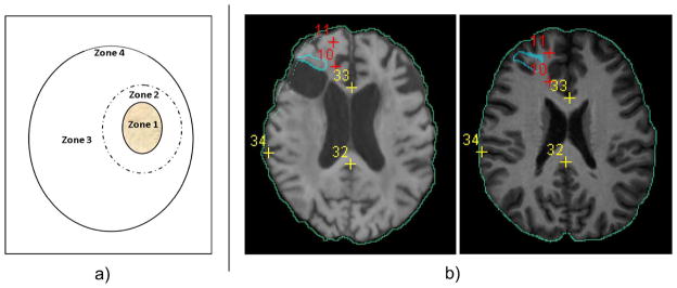
Measuring registration accuracies in different zones. Panel (a) is the sketch of dividing the whole images into various zones. The solid contour filled with yellow texture denotes the abnormal zone (Zone 1), which contains the post-resection cavity and the recurrent tumor. Zones 2 and 3 are normal-appearing regions immediately close to, and far away from, Zone 1. Zone 4 is the whole brain boundary. The definition of the zones can be found in the main context in Section III-D4. Panel (b) shows landmark/ROI definitions for an example pair of images. Blue contours are expert-defined ROIs in Zone 1. Red crosses are expert-defined landmarks in Zone 2. Yellow crosses are expert-defined landmarks in Zone 3. Green contours are the automatically-computed brain boundaries (through Canny edge detection of the brain masks), to measure the registration accuracy in Zone 4. Please note that the landmark/ROI definitions from a second expert (which are not shown here) may differ. This figure is best viewed in color.

• Zone 1: Abnormal region. Experts HA and MB together contoured the abnormal region that contains 1) the post-resection cavity and 2) the recurred tumor. Within this contour was what we defined as Zone 1, the abnormal region [see Fig. 5(a)]. The experts referred to FLuid-Attenuated Inversion-Recovery (FLAIR) MR image for this contouring, because of its high sensitivity and specificity in delineating brain tumors [69]–[71]. Then they independently found the corresponding regions in the normal template image. We measured the accuracy of registration in Zone 1 by two metrics: 1) the average Dice overlap, and 2) the 95-th percentile Hausdorff Distance, between the algorithm-warped abnormal region and two rater-warped abnormal regions in the template space. A higher regional overlap and a smaller distance reflect a better alignment of two images in Zone 1.

• Zone 2: Regions immediately neighboring the abnormal region. A 30 mm-wide band immediately outside the abnormal region was defined, by morphologically dilating the abnormal region mask agreed by the two experts in the patient’s image space [see Fig. 5(a)]. Anatomical landmarks were identified in this band, which served as the references to reflect the registration accuracy in the immediate neighborhood of abnormalities. One expert (HA) labeled 10 anatomical landmarks in Zone 2 within the patient image. The two experts then independently labeled the corresponding anatomical landmarks in the template space. The average Euclidean distance between the algorithm-calculated corresponding landmark locations and the rater-labeled corresponding landmark locations in the template space was used to measure the registration accuracy in Zone 2. Smaller landmark errors point to higher registration accuracy. The concept is depicted in Fig. 6. Given a set of expert-annotated landmarks ${\{x_n\}}_{n=1}^N$ in the patient image, their corresponding landmark locations ${\{y_n^{\text{expert}1}\}}_{n=1}^N$ (independently by expert HA) and ${\{y_n^{\text{expert}2}\}}_{n=1}^N$ (independently by expert MB) in the template image, and the algorithm-calculated corresponding landmark locations ${\{y_n^{\text{algorithm}}\}}_{n=1}^N$ also in the template image, we defined the inter-expert landmark errors (the length of the solid line in Fig. 6) as

  $$d(y_n^{\text{expert}1},y_n^{\text{expert}2}),\text{for}n=1,2,\dots ,N$$ (3)
  and the algorithm-to-expert landmark errors (the average length of the dashed lines in Fig. 6) as

  $$\frac{1}{2}[d(y_n^{\text{algorithm}},y_n^{\text{expert}1})+d(y_n^{\text{algorithm}},y_n^{\text{expert}2})],\forall n$$ (4)

  where d(·,·) is the Euclidean distance between two voxel locations.

• Zone 3: Regions far away from the abnormal region. Zone 3 was defined as all the normal regions outside Zone 2 [see Fig. 5(a)]. We used landmarks to evaluate the registration accuracy in Zone 3. This could show how the recurrent tumor and the cavities have influenced registration in faraway normal-appearing regions. One expert (HA) labeled 40 anatomical landmarks in Zone 3. Then two experts independently labeled corresponding landmarks in the template space. Registration accuracy in this zone was measured by the average Euclidean distance between the algorithm-calculated corresponding landmarks and the rater-labeled corresponding landmarks in the template space. Smaller landmark errors point to higher registration accuracy in Zone 3.

• Zone 4: Brain boundaries. The existence of cavities and recurrent tumors inside the patient image may even influence the alignment of the brain boundaries between the patient and the normal-appearing template images. To capture this influence, we measured the dice overlap and the 95th percentile Hausdorff Distance between the warped and the template brain masks. A higher dice overlap and smaller distance indicate a higher level of robustness of a registration algorithm with regard to the abnormality-induced negative impact.

Fig. 6.

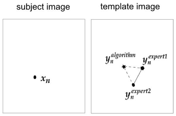
Depiction of inter-expert and algorithm versus expert landmark errors.

IV. Results and Analysis

In this section, we use four subsections to present the evaluation results in the databases representing the four aforementioned challenges.

A. Results in Databases Representing Challenge 1

Fig. 7 shows the average Jaccard overlap over all ROIs in the NIREP and LONI-LPBA40 databases. A detailed table of Jaccard overlap per ROI can be found in Appendix C for all algorithms evaluated in this paper. Several observations can be made from this set of results.

Fig. 7.

Box-and-Whisker plots of registration accuracies in the NIREP and LONI-LPBA40 databases, as indicated by the Jaccard overlaps averaged across 32 (in NIREP) or 56 (in LONI-LPBA40) ROIs. This figure shows how registration methods perform facing Challenge 1 (inter-subject variability).

1. DRAMMS and ANTs obtained the highest Jaccard overlaps in both databases. Between the two methods, DRAMMS had a slightly higher accuracy in the NIREP database (Jaccard = 0.5249 ± 0.0254 for ANTs and 0.5292 ± 0.0266 for DRAMMS, p = 0.0687); whereas ANTs had a slightly higher accuracy in the LONI-LPBA40 database (Jaccard = 0.5710 ± 0.0161 for ANTs and 0.5666 ± 0.0163 for DRAMMS, p = 0.0188). In both cases, the differences were tiny (<0.005 difference between the average Jaccard overlaps in the 0–1 scale). Following ANTs/DRAMMS were DROP, Demons and ART registration methods. Among these methods, ANTs and ART were included in the evaluation study [17] and were found to be the two most accurate methods. Our findings here showed a similar trend. In addition, the three methods—DRAMMS, DROP and (the nondiffeomorphic, or additive, version of) Demons, which were not included in [17], showed highly competitive performances.

2. Methods such as SSD-FFD, fnirt, DROP use intensity differences (SSD) as the similarity metric. On average, they had reasonable Jaccard overlaps. However, they also showed larger variations of regional overlaps, and therefore they were less stable in our experiments than those methods using CC, MI, or attribute-based similarity measures.

3. The high degree of freedom allowed by a deformation mechanism (such as the FFD model as used in DRAMMS and the diffeomorphism LDDMM model as used in ANTs) is perhaps another factor contributing to the higher registration accuracy, compared to deformation mechanisms with relatively few degrees of freedom (such as fifth-order polynomials in AIR).

B. Results in Databases Representing Challenge 2

For the three databases containing raw images, we had two scenarios—one focusing on the localized structures and tissue types throughout the image space (the BrainWeb database); and the second scenario focusing on the brain masks (the IBSR and OASIS databases), which is crucial for (multi-)atlas-based skull-stripping.

Scenario 1. Registration Accuracy in Multiple Localized ROIs/Structures in the Raw Images

Fig. 8 shows the average Jaccard overlaps of the 11 ROIs in the BrainWeb database. Several observations can be made.

Fig. 8.

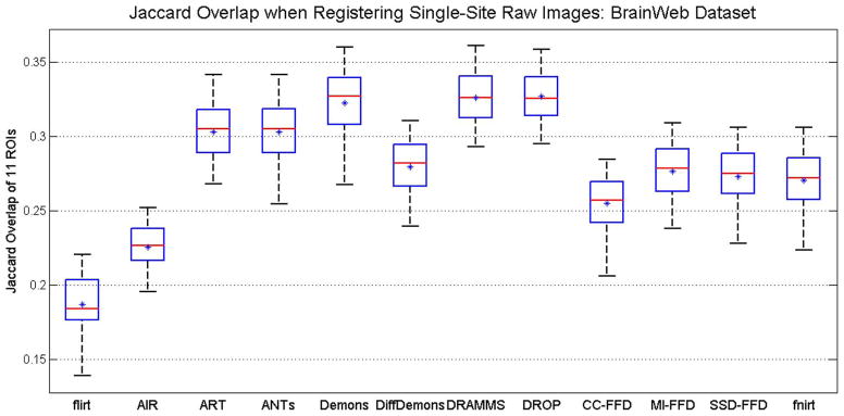
Box-and-Whisker plots of registration accuracy in the BrainWeb database, as indicated by the Jaccard overlaps averaged across 11 available ROIs. This is Scenario 1 in the testing of registration methods facing Challenge 2 (intensity inhomogeneity, noise and structural differences in raw images).

1. DRAMMS, DROP and Demons obtained similarly high accuracies, followed closely by the ANTs and ART methods. These registration methods were also among the most accurate ones in registering skull-stripped brain images as shown in the previous sub-section.

2. On the other hand, the average Jaccard overlap in various ROIs by the best-performing algorithm in this raw, with-skull database (i.e., DRAMMS) was only around 0.32 (Fig. 8). Compared to the average Jaccard of 0.52–0.57 in registering skull-stripped brain images (Fig. 7), this clearly underlined the increased level of difficulty in registering raw, with-skull brain images.

Scenario 2. Registration Accuracy in Brain Masks of the Raw Images

In this registration scenario, we focused on the accuracy of registration in warping the brain masks, which is the basis for the atlas-based skull-stripping framework (e.g., [19], [25]). Fig. 9 shows the accuracies of three registration methods (ANTs, Demons and DRAMMS), which were forerunners in the results in Scenario 1. Several observations can be made.

Fig. 9.

Registration accuracy in raw brain images, in the IBSR and OASIS databases, as indicated by the Jaccard overlap (the first row) and 95th percentile Hausdorff Distance (the second row), between the warped and the target brain masks. This is Scenario 2 in the testing of registration methods facing Challenge 2 (intensity inhomogeneity, noise and structural differences in raw images). “prctile” in the title of the second subfigure means “percentile”.

1. The Jaccard regional overlap and the 95th percentile Hausdorff Distance showed the same trend for aligning the brain masks—a higher Jaccard overlap corresponded to a smaller distance;

2. The ranking and the difference of methods seemed to be highly dependent on the database, especially the level of difficulty for registration in a database. In the OASIS database, which exhibits a lower level of inter-subject FOV differences and intensity inhomogeneity [as can be seen in Fig. 2(c)], ANTs scored the highest accuracy, followed closely by Demons and DRAMMS. In the IBSR database, however, which exhibits a higher level of inhomogeneity, background noise and larger deformations, DRAMMS scored the highest accuracy, followed, with relatively bigger distances, by Demons and ANTs.

3. Overall, a Jaccard overlap of 0.75–0.93 could be expected for the brain masks when we registered raw, with-skull images within a same database. This should provide a promising starting point for (multi-)atlas-based skull-stripping (e.g., [19], [25]). On the other hand, one needs to be aware that the registration accuracy might decrease when images are from multi-site databases, usually with larger imaging and FOV differences (to be shown in the next subsection).

C. Results in the Database Representing Challenge 3

Fig. 10 shows the overlap results averaged over all 90 pair-wise inter-subject registrations in the ADNI database. Compared to the registration within the single-site database, the registration of raw images acquired from multiple imaging sites encountered an increased level of difficulty. Specifically, three observations can be made.

Fig. 10.

Jaccard overlaps in the ADNI database, for a) the brain mask (the left three columns); b) the left hippocampus (the middle three columns); and c) the right hippocampus (the right three columns). This figure shows how registration methods perform in a typical multi-site database, where additional challenges arise from the imaging and FOV differences in different imaging institutions (Challenge 3).

1. DRAMMS and ANTs performed better than Demons in aligning the brain masks. They showed higher levels of robustness with regard to the FOV differences, the background noise and the presence of skull or other nonbrain structures.

2. The presence of the skull, the background noise, and especially the FOV difference, in the ADNI multi-site database, had a clearly visible impact on the accuracy of aligning deep brain structures. When registering skull-stripped images from single-site databases such as in the LONI-LPBA40 database, ANTs, Demons and DRAMMS could align hippocampi at Jaccard overlaps around 0.6, and they differed by less than 0.05 Jaccard overlap on average (see Table V in Appendix C). However, when the raw images from the multi-site ADNI database were used, even the best-performing algorithms (DRAMMS and Demons as shown in Fig. 10) could only align hippocampi at Jaccard overlaps around 0.5 on average, and algorithms had greater differences in terms of the Jaccard overlaps they obtained. Another factor that caused the decrease in the accuracy and the increase in the differences among methods could be that those subjects in the ADNI database have highly variable degrees of neuro-degeneration (three normal controls, four MCI, and three AD subjects), and hence they have largely different ventricle sizes, atrophy patterns, and hippocampus sizes (see Fig. 11 for some examples of very difficult cases, which will be described in item 4 below).

3. Considering the quantitative results in all three regions (brain mask, left, and right hippocampi) in those with-skull raw images acquired from multiple institutions, DRAMMS showed the greatest promise.

4. Besides the quantitative results in the limited number of structures such as the brain masks and the hippocampi, the visual inspection of the registration results in the whole images could actually reveal much greater differences among registration methods. Fig. 11 shows some registration results from Demons, ANTs and DRAMMS in two pairs of subjects from the multi-site ADNI database. As pointed out by blue arrows in the figure, DRAMMS showed a clear advantage to align the largely different anatomies such as the ventricles. To capture this large difference, many algorithms may have to increase their search ranges. However, this usually requires considerable efforts for task-specific, or even individual-specific, parameter adjustments. Adjusting search ranges is a non-trivial research topic. It often requires specific theoretic designs [73], or requires the introduction of anatomical landmarks [74]–[80]. The main difficulty is to effectively balance between capturing the large differences and capturing the local subtle displacements. Therefore, algorithms that can capture and balance between both, and do not require additional parameter adjustments, become favorable. Actually, in our recent studies that spatially normalized all 800+ ADNI subjects into a common template (from a normal control subject), a small portion of the Alzheimer’s Disease (AD) subjects have unusually large ventricles than many other AD subjects. We considered a registration “failure” if there were more than 5 mm errors in the ventricle boundaries (visually pronounced errors). Accordingly, the success rate was defined by

   $$1-\frac{(\#(\text{failed}\text{pair}-\text{wise}\text{registration}))}{(\#(\text{all}\text{pair}-\text{wise}\text{registration}))}.$$

   Compared to the 80%–85% success rate by ANTs and Demons when used with the fixed sets of parameters, DRAMMS, also using a fixed set of parameters as in other cases, achieved a success rate of 96%, which was a clear improvement of registration accuracy in this large-scale multi-institutional database.

TABLE V.

Jaccard Overlap for Each of the 56 ROIs in the LONI-LPBA40 Database, Averaged Among All 210 Registrations (×10⁻²). For Each ROI, Bold Texts and Light-Gray Texts Indicate That the Corresponding Registration Methods Obtain the Highest and the Second Highest Overlap Compared to Other Registration Methods

	flirt	AIR	ART	ANTs	Demons	DiffDemons	DRAMMS	DROP	CC-FFD	MI-FFD	SSD-FFD	fnirt
L superior frontal gyrus	62.3 ± 4.8	65.5 ± 4.1	67.7 ± 4.8	69.5 ± 4.7	68.7 ± 4.7	69.0 ± 4.8	69.0 ± 4.7	68.1 ± 5.3	66.3 ± 4.7	66.2 ± 5.1	66.6 ± 6.3	56.1 ± 6.4
R superior frontal gyrus	62.3 ± 3.8	64.0 ± 4.2	66.5 ± 4.8	69.4 ± 4.2	68.3 ± 4.0	68.8 ± 4.0	68.6 ± 4.4	67.8 ± 4.3	65.6 ± 3.9	65.4 ± 4.6	66.1 ± 4.7	51.0 ± 8.8
L middle frontal gyrus	58.8 ± 5.6	61.0 ± 4.8	62.6 ± 5.7	64.6 ± 5.9	63.3 ± 5.4	63.7 ± 5.5	64.1 ± 5.9	62.7 ± 5.5	61.8 ± 5.2	62.2 ± 5.3	62.7 ± 5.3	52.6 ± 7.0
R middle frontal gyrus	59.8 ± 5.5	60.2 ± 5.8	61.9 ± 6.3	64.9 ± 5.8	63.7 ± 5.6	64.1 ± 5.7	64.2 ± 6.0	62.8 ± 5.6	62.1 ± 5.4	62.7 ± 5.4	62.8 ± 5.5	45.7 ± 10.8
L inferior frontal gyrus	52.0 ± 6.1	55.5 ± 5.5	57.8 ± 6.8	59.5 ± 7.2	59.0 ± 6.7	59.4 ± 6.8	59.4 ± 6.9	58.8 ± 7.1	55.7 ± 6.5	56.6 ± 7.0	57.6 ± 7.0	51.1 ± 6.5
R inferior frontal gyrus	52.4 ± 7.7	53.6 ± 6.8	55.9 ± 7.6	57.8 ± 8.7	57.3 ± 7.7	57.5 ± 7.8	57.2 ± 8.3	56.8 ± 8.0	55.4 ± 7.4	56.3 ± 7.2	56.4 ± 7.8	47.1 ± 7.8
L precentral gyrus	48.3 ± 7.7	50.4 ± 7.6	56.7 ± 9.3	62.3 ± 8.7	59.4 ± 7.5	60.6 ± 7.4	61.8 ± 8.3	59.8 ± 7.8	50.0 ± 8.1	53.5 ± 9.0	54.4 ± 9.1	46.4 ± 8.2
R precentral gyrus	49.0 ± 6.1	50.0 ± 6.5	53.3 ± 8.6	61.0 ± 5.9	59.4 ± 5.5	60.4 ± 5.4	61.0 ± 6.6	57.5 ± 7.0	50.9 ± 6.3	53.8 ± 7.0	53.9 ± 7.8	42.4 ± 9.8
L middle orbitofrontal gyrus	44.0 ± 8.5	49.0 ± 7.6	52.8 ± 8.1	53.7 ± 8.8	53.3 ± 8.7	53.6 ± 8.8	53.4 ± 8.6	53.0 ± 8.5	49.8 ± 8.8	51.0 ± 8.6	52.5 ± 8.5	41.6 ± 10.0
R middle orbitofrontal gyrus	44.7 ± 8.6	48.3 ± 8.8	50.9 ± 8.8	52.4 ± 9.1	52.0 ± 9.2	52.2 ± 9.3	52.3 ± 8.9	52.0 ± 8.7	49.4 ± 9.2	49.0 ± 9.3	50.4 ± 9.1	36.3 ± 9.2
L lateral orbitofrontal gyrus	39.2 ± 7.2	43.0 ± 6.3	48.1 ± 7.7	49.5 ± 7.7	48.5 ± 6.9	49.0 ± 6.9	49.4 ± 7.5	47.6 ± 7.6	45.1 ± 6.3	45.7 ± 7.5	47.2 ± 6.7	36.9 ± 8.7
R lateral orbitofrontal gyrus	36.0 ± 8.1	39.4 ± 6.8	43.5 ± 7.8	44.1 ± 9.1	43.2 ± 8.4	43.5 ± 8.6	44.1 ± 8.9	43.3 ± 8.0	40.6 ± 7.6	40.7 ± 8.2	41.5 ± 7.8	30.7 ± 8.9
L gyrus rectus	43.8 ± 7.5	47.7 ± 6.9	50.2 ± 7.9	53.2 ± 6.8	52.9 ± 5.8	53.3 ± 5.8	52.4 ± 7.0	52.9 ± 6.7	47.0 ± 7.1	47.1 ± 7.1	50.7 ± 6.8	44.5 ± 7.2
R gyrus rectus	44.3 ± 7.9	48.7 ± 6.5	51.9 ± 7.8	54.5 ± 7.1	53.2 ± 6.9	53.5 ± 7.0	53.9 ± 7.3	53.7 ± 7.0	47.9 ± 7.0	47.9 ± 8.4	50.2 ± 7.2	43.7 ± 9.4
L postcentral gyrus	39.7 ± 8.9	44.0 ± 8.0	47.8 ± 11.6	54.3 ± 10.9	50.9 ± 10.0	52.3 ± 9.9	53.5 ± 11.1	50.9 ± 10.6	41.9 ± 9.8	45.4 ± 11.0	46.1 ± 11.2	41.8 ± 8.3
R postcentral gyrus	41.9 ± 6.7	44.3 ± 7.0	46.1 ± 10.7	56.4 ± 8.3	53.4 ± 7.6	54.7 ± 7.5	56.0 ± 8.4	51.4 ± 9.4	43.9 ± 7.4	47.1 ± 8.4	47.8 ± 9.8	41.2 ± 8.5
L superior parietal gyrus	51.8 ± 4.9	52.2 ± 5.8	54.1 ± 6.6	58.9 ± 5.8	57.0 ± 5.1	57.5 ± 5.2	58.1 ± 5.5	56.4 ± 5.7	53.9 ± 5.2	54.2 ± 5.7	55.6 ± 5.3	43.9 ± 8.2
R superior parietal gyrus	52.7 ± 5.4	53.4 ± 5.6	53.4 ± 7.1	59.8 ± 6.2	58.4 ± 5.7	58.9 ± 5.8	58.4 ± 6.3	57.1 ± 6.5	55.3 ± 5.5	55.8 ± 6.1	57.2 ± 5.9	41.6 ± 8.7
L supramarginal gyrus	42.0 ± 7.3	43.6 ± 7.7	45.9 ± 8.6	50.3 ± 7.2	49.0 ± 6.8	49.9 ± 6.9	48.9 ± 7.6	48.8 ± 7.2	43.8 ± 7.0	45.9 ± 7.3	47.2 ± 7.0	40.4 ± 7.9
R supramarginal gyrus	40.8 ± 8.6	41.4 ± 7.8	41.2 ± 10.6	47.0 ± 9.9	46.3 ± 9.2	46.9 ± 9.3	46.4 ± 10.0	44.7 ± 10.1	41.4 ± 8.5	42.2 ± 9.8	44.2 ± 9.5	38.9 ± 8.7
L angular gyrus	42.3 ± 10.5	41.6 ± 9.7	43.2 ± 11.5	46.9 ± 11.2	45.7 ± 10.6	46.2 ± 10.7	46.3 ± 11.2	45.1 ± 11.3	42.9 ± 10.3	42.7 ± 10.2	44.4 ± 10.8	36.7 ± 10.1
R angular gyrus	44.8 ± 5.7	45.5 ± 8.0	44.7 ± 8.8	49.7 ± 6.4	49.7 ± 6.3	50.0 ± 6.3	49.3 ± 6.8	48.9 ± 6.6	46.9 ± 6.2	46.5 ± 6.4	48.3 ± 6.7	38.9 ± 8.0
L precuneus	45.4 ± 5.8	45.3 ± 6.0	48.0 ± 6.2	50.4 ± 5.8	49.8 ± 5.4	49.9 ± 5.5	49.8 ± 5.9	48.7 ± 5.9	47.1 ± 5.4	46.8 ± 5.7	47.1 ± 5.8	43.1 ± 6.6
R precuneus	47.5 ± 6.4	49.1 ± 6.2	50.9 ± 6.5	53.9 ± 6.1	52.9 ± 6.4	53.0 ± 6.3	53.0 ± 6.1	52.0 ± 6.9	49.7 ± 6.4	49.9 ± 7.0	49.8 ± 7.2	44.2 ± 7.5
L superior occipital gyrus	37.7 ± 8.7	39.4 ± 8.4	40.7 ± 10.5	45.5 ± 10.3	44.4 ± 9.7	44.7 ± 9.9	43.9 ± 10.7	43.2 ± 10.6	40.3 ± 8.8	41.2 ± 9.4	42.7 ± 9.8	33.5 ± 9.8
R superior occipital gyrus	35.6 ± 7.8	36.4 ± 9.2	38.1 ± 10.2	43.2 ± 10.3	42.0 ± 9.5	42.4 ± 9.8	41.8 ± 10.8	41.1 ± 10.3	38.5 ± 8.5	39.6 ± 9.3	40.9 ± 9.4	30.8 ± 10.0
L middle occipital gyrus	47.6 ± 7.0	47.0 ± 7.8	49.7 ± 7.9	52.5 ± 7.0	51.8 ± 6.7	52.2 ± 6.8	51.7 ± 7.3	51.3 ± 7.2	49.9 ± 6.9	49.8 ± 7.2	50.8 ± 7.0	43.4 ± 7.0
R middle occipital gyrus	47.9 ± 6.1	48.6 ± 6.4	50.6 ± 7.4	54.3 ± 6.5	53.6 ± 6.3	53.9 ± 6.3	53.6 ± 6.1	52.9 ± 6.4	51.2 ± 6.5	50.6 ± 6.9	52.3 ± 6.7	44.6 ± 6.3
L inferior occipital gyrus	43.7 ± 7.9	45.9 ± 8.7	49.1 ± 8.0	51.6 ± 7.5	50.7 ± 7.3	51.0 ± 7.3	51.5 ± 7.8	50.8 ± 7.8	48.6 ± 7.6	48.2 ± 8.0	50.3 ± 7.4	38.1 ± 9.2
R inferior occipital gyrus	43.8 ± 8.3	49.6 ± 7.4	50.6 ± 7.4	53.9 ± 8.2	53.4 ± 7.8	53.8 ± 7.8	53.9 ± 8.1	52.5 ± 7.9	51.3 ± 7.8	50.7 ± 7.9	52.0 ± 7.9	40.3 ± 9.3
L cuneus	43.0 ± 11.5	44.3 ± 10.0	47.1 ± 8.8	50.7 ± 9.9	49.9 ± 9.5	50.2 ± 9.6	49.9 ± 9.7	48.2 ± 9.6	47.1 ± 9.5	45.5 ± 9.6	46.1 ± 10.2	40.6 ± 8.8
R cuneus	40.4 ± 10.2	44.6 ± 10.2	46.3 ± 9.9	49.3 ± 11.5	48.8 ± 10.7	49.3 ± 10.7	48.2 ± 11.1	47.6 ± 12.2	44.5 ± 10.2	44.8 ± 10.8	45.7 ± 11.7	40.5 ± 10.1
L superior temporal gyrus	49.3 ± 5.5	53.5 ± 4.2	60.6 ± 5.1	63.9 ± 4.3	61.8 ± 4.1	62.6 ± 4.2	63.3 ± 4.4	62.4 ± 4.6	55.4 ± 4.2	59.8 ± 4.3	60.1 ± 4.3	51.9 ± 5.3
R superior temporal gyrus	51.1 ± 5.4	54.2 ± 4.1	59.7 ± 5.5	63.5 ± 4.9	61.8 ± 4.7	62.5 ± 4.8	63.4 ± 5.0	61.8 ± 5.3	55.8 ± 4.8	59.2 ± 5.2	60.3 ± 4.8	51.5 ± 5.5
L middle temporal gyrus	42.9 ± 5.5	47.0 ± 5.5	48.5 ± 5.6	52.3 ± 5.5	51.0 ± 5.0	51.5 ± 5.2	51.5 ± 5.4	50.4 ± 5.9	47.0 ± 5.3	48.1 ± 5.8	49.2 ± 5.5	43.9 ± 5.9
R middle temporal gyrus	45.3 ± 6.2	47.7 ± 5.9	49.7 ± 6.3	54.6 ± 6.0	53.1 ± 5.9	53.7 ± 6.0	53.3 ± 6.2	52.5 ± 6.2	48.3 ± 5.6	49.7 ± 6.0	51.5 ± 5.8	46.6 ± 6.6
L inferior temporal gyrus	42.1 ± 6.5	45.1 ± 6.9	48.6 ± 7.0	51.9 ± 7.8	50.7 ± 7.3	51.1 ± 7.4	50.9 ± 7.7	50.0 ± 7.7	47.7 ± 7.0	48.0 ± 7.2	49.3 ± 7.5	40.6 ± 7.0
R inferior temporal gyrus	43.9 ± 6.1	45.5 ± 6.6	49.8 ± 6.1	53.5 ± 6.2	52.3 ± 6.2	52.6 ± 6.3	52.2 ± 6.1	51.4 ± 6.2	49.6 ± 6.0	50.0 ± 6.3	51.0 ± 6.3	42.7 ± 6.6
L parahippocampal gyrus	43.2 ± 6.5	46.9 ± 5.9	53.4 ± 7.0	55.6 ± 6.3	53.5 ± 6.0	54.1 ± 6.1	56.2 ± 6.1	53.1 ± 6.9	46.9 ± 6.1	48.1 ± 6.9	48.9 ± 7.8	37.8 ± 8.9
R parahippocampal gyrus	45.0 ± 6.4	46.4 ± 6.3	52.4 ± 6.3	56.0 ± 5.7	54.2 ± 5.9	54.8 ± 5.8	55.8 ± 5.5	53.1 ± 6.5	46.7 ± 6.6	48.0 ± 7.1	48.5 ± 8.2	35.2 ± 10.9
L lingual gyrus	48.8 ± 6.1	49.7 ± 5.8	56.3 ± 6.0	58.8 ± 6.2	57.2 ± 5.7	57.9 ± 5.9	58.0 ± 6.3	56.3 ± 6.5	51.4 ± 5.5	52.2 ± 6.2	52.7 ± 6.5	47.1 ± 7.5
R lingual gyrus	49.5 ± 6.9	54.4 ± 4.7	57.7 ± 6.6	61.2 ± 5.9	60.2 ± 5.2	60.9 ± 5.5	60.2 ± 6.2	59.0 ± 6.1	54.4 ± 5.6	55.5 ± 5.9	56.0 ± 5.9	48.1 ± 7.9
L fusiform gyrus	47.7 ± 5.9	49.3 ± 7.5	53.8 ± 7.2	56.7 ± 6.3	55.2 ± 6.1	55.8 ± 6.3	56.5 ± 6.7	54.3 ± 6.9	50.7 ± 6.0	50.6 ± 6.6	52.6 ± 6.4	44.5 ± 7.3
R fusiform gyrus	48.4 ± 5.3	51.0 ± 5.2	55.4 ± 5.8	58.4 ± 5.8	56.8 ± 5.7	57.3 ± 6.0	58.0 ± 5.6	56.3 ± 6.0	52.0 ± 5.0	52.8 ± 6.3	53.8 ± 6.0	44.8 ± 6.9
L insular cortex	54.5 ± 6.3	55.2 ± 6.5	68.4 ± 3.2	69.0 ± 3.2	65.3 ± 3.3	65.8 ± 3.2	68.7 ± 3.0	62.5 ± 7.1	57.5 ± 4.6	62.2 ± 3.8	59.6 ± 7.3	60.2 ± 4.2
R insular cortex	53.2 ± 5.7	53.7 ± 5.6	66.1 ± 4.6	66.9 ± 5.2	61.6 ± 5.1	62.3 ± 5.2	65.7 ± 5.0	59.3 ± 7.2	55.4 ± 4.7	57.9 ± 5.2	55.8 ± 7.4	57.2 ± 5.3
L cingulate gyrus	44.6 ± 6.1	47.5 ± 5.6	55.2 ± 6.0	56.0 ± 6.4	53.4 ± 5.5	53.6 ± 5.7	55.3 ± 6.0	52.4 ± 6.1	47.3 ± 5.9	48.6 ± 6.4	47.7 ± 6.8	47.6 ± 8.4
R cingulate gyrus	47.3 ± 7.0	46.9 ± 7.4	54.6 ± 8.7	55.5 ± 8.8	53.1 ± 8.4	53.5 ± 8.5	54.6 ± 8.3	51.6 ± 8.9	47.8 ± 7.4	47.9 ± 8.0	47.4 ± 8.7	47.2 ± 9.0
L caudate	47.5 ± 11.1	46.3 ± 13.1	58.7 ± 9.0	59.0 ± 8.8	55.5 ± 9.9	56.1 ± 10.1	62.1 ± 7.6	54.1 ± 10.7	52.1 ± 9.4	54.1 ± 8.5	48.0 ± 12.6	49.1 ± 11.6
R caudate	47.1 ± 9.8	46.2 ± 12.1	58.0 ± 9.1	57.0 ± 10.2	53.2 ± 11.5	53.7 ± 11.8	60.1 ± 8.2	52.8 ± 12.2	51.8 ± 8.9	52.9 ± 9.2	47.4 ± 13.2	48.9 ± 11.5
L putamen	56.1 ± 5.9	56.7 ± 5.7	66.1 ± 3.6	67.4 ± 3.5	60.0 ± 6.7	59.9 ± 7.2	67.0 ± 3.5	51.2 ± 14.7	57.6 ± 5.0	55.8 ± 6.7	50.5 ± 13.5	60.4 ± 5.5
R putamen	57.8 ± 5.9	56.1 ± 6.8	64.9 ± 5.1	65.5 ± 5.1	57.0 ± 8.8	57.1 ± 9.2	65.0 ± 5.2	48.7 ± 15.5	57.6 ± 6.1	53.3 ± 8.4	48.7 ± 15.0	57.5 ± 6.4
L hippocampus	49.3 ± 10.1	53.7 ± 7.2	61.4 ± 5.1	63.1 ± 4.8	60.1 ± 6.5	60.1 ± 6.6	62.6 ± 5.1	57.9 ± 8.6	51.3 ± 8.8	52.6 ± 10.9	52.3 ± 11.9	51.0 ± 8.5
R hippocampus	49.2 ± 8.6	51.0 ± 7.6	58.2 ± 6.3	60.3 ± 5.3	57.8 ± 7.2	58.1 ± 7.2	60.8 ± 5.1	55.5 ± 9.9	49.3 ± 10.4	50.7 ± 12.9	49.1 ± 14.5	47.2 ± 10.1
cerebellum	74.9 ± 3.8	57.8 ± 7.8	76.7 ± 3.5	77.4 ± 3.7	77.2 ± 3.6	77.3 ± 3.6	77.9 ± 3.5	77.4 ± 3.5	76.8 ± 3.7	73.0 ± 4.7	77.0 ± 3.6	69.5 ± 5.7
brainstem	66.3 ± 9.4	54.7 ± 8.3	68.0 ± 8.3	68.9 ± 7.9	68.2 ± 7.6	67.9 ± 7.7	68.5 ± 7.6	67.2 ± 7.5	66.9 ± 8.4	62.5 ± 8.2	67.2 ± 7.5	63.9 ± 7.2

Fig. 11.

Demons, ANTs and DRAMMS registration results of two pairs of images having large anatomical variations especially in ventricles, mainly due to their different levels of neuro-degeneration. All subjects are from the multi-site ADNI database. Blue arrows point to some typical locations where registration results from three methods differ greatly.

D. Results in Database Representing Challenge 4

Fig. 12 shows the quantitative registration errors in the pathology-to-normal subject registration. As a reference, this figure also includes inter-expert errors between the two independent experts in Zones 1–3. A desirable registration should 1) accurately register the normal-appearing regions, where correspondences can be established (i.e., small landmark errors in Zone 2–3); 2) accurately align the brain boundaries (i.e., small 95%-percentile HD distances in Zone 4); and 3) map the pathological regions to the right location but relax the deformation within the pathological regions, where correspondences could hardly be established (i.e., high regional overlaps in Zone 1). In Fig. 12, several observations can be made.

Fig. 12.

Landmark errors or the 95th percentile Hausdorff Distance in various zones in the pathology-to-normal subject registrations. In addition to the errors, we have shown the average Jaccard overlap in Zone 1 in this figure. This figure shows how registration methods perform in the presence of pathology-induced missing correspondences (Challenge 4).

1. Two independent experts agreed with each other only at a 0.48 Jaccard overlap on average in the cavity and tumor recurrence regions (Zone 1). This reflected the difficulty, or the ambiguity, for the human experts to deal with the missing correspondences. Among the four methods evaluated, ANTs agreed with experts at the highest level (average Jaccard 0.40), followed closely by DRAMMS (average 0.37 Jaccard overlap). The 95th percentile Hausdorff Distances showed the same trend. Overall, experts showed better agreement between each other than between algorithms and experts.

2. In Zone 2 (the immediate neighborhood of the abnormal regions), the average landmark error was 4.1 mm between experts. Landmarks errors for DRAMMS, ANTs and Diffeomorphic Demons were similar (at 3.9, 4.1, and 4.4 mm, respectively), and also comparable to the inter-expert errors.

3. Further away from the abnormal regions, Zone 3 had larger landmark errors than Zone 2. The average errors were 5.3 mm between experts, 5.8 mm for DRAMMS, and 5.9 mm for ANTs. Diffeomorphic Demons and especially fnirt started to have larger landmark errors (6.6 and 9.6 mm on average). This difference may, in part, be attributed to the fact that DRAMMS used texture features and ANTs used correlation coefficient as similarity metric, which were perhaps more robust and reliable than the intensity difference which Demons and fnirt used as their similarity metrics.

4. Another interesting finding was in Zone 4 (brain boundary). Because of the sharp contrast between foreground and background in a skull-stripped image, the brain boundaries ought to be among the easiest parts to register. In the presence of pathologies, however, this was surprisingly not always the case. Fnirt, for example, had 11.1 mm as the 95th percentile Hausdorff Distance at brain boundaries, which meant registration failures in several cases. ANTs had, on average, 3.3 mm as the 95th percentile Hausdorff Distance in the brain boundary, which was even bigger than the average errors ANTs produced in the abnormal regions (2.1 mm). By carefully examining the output images, we found that this average boundary error by ANTs was mainly caused by misalignments in the boundaries close to the pathology sites in several cases. This showed that the pathology regions may impact a wide area in ANTs registration. On the other hand, DRAMMS and Diffeomorphic Demons had the smallest boundary errors (1.8 and 2.2 mm, respectively). Both errors were smaller than those in the abnormal regions, indicating good alignments of the brain boundaries. This showed that the negative effect of pathological regions was more localized in DRAMMS and Diffeomorphic Demons registration algorithms, which should be desirable.

It should be emphasized that general-purpose registration algorithms are usually not designed for registering pathology-bearing images. Task-specific registration algorithms are often needed to segment and specifically deal with the pathology-affected regions. However, the fact that DRAMMS, as a general-purpose registration algorithm, performed stably and robustly in all Zones 1–4, highlighted the effect of using attributes to measure voxel similarities and to quantify voxel-wise matching reliabilities. To better illustrate this, Fig. 13 shows a set of representative DRAMMS registration results (registration from a tumor-recurring patient’s brain image to the normal-appearing brain template image). First, DRAMMS extracted high-dimensional Gabor texture attributes to represent each voxel. The attributes should be more informative than intensities in the search for correspondences. Moreover, at each voxel, DRAMMS automatically calculated a so-called “mutual-saliency” weight, also based on the attributes. The mutual-saliency quantified the chance of each and every voxel to establish a reliable correspondence between the two images. As Fig. 13(d) shows, the mutual-saliency map effectively identified outlier regions (dark blue), where correspondences could be hardly established. The identified outlier regions coincided with the recurrent tumor regions [as red arrows pointed out in panel (a)]. Note that, this was obtained without any segmentation, manual masking, or any prior knowledge of the presence or the location of the tumor recurrence. Being segmentation-free is a feature that differentiates DRAMMS from those task-specific cost-function-masking approaches or pathology-seeding approaches. As a result of this attribute-based similarity measurement and mutual-saliency weighting, the registration by DRAMMS was mainly driven by the regions where correspondences could be well established. This led to visually plausible results as shown in Fig. 13(c).

Fig. 13.

Registration of a brain image with tumor recurrence to a normal brain template by DRAMMS, for a series of slices in the coronal view. This figures shows how the mutual-saliency mechanism (a spatial-varying utilization of voxels) helped DRAMMS in the pathological-to-normal subject registration scenario. Without segmentation, initialization, or prior knowledge, the automatically-calculated mutual-saliency map (d), defined in the target image space, effectively assigned low weights to those regions that correspond to those outlier regions (pointed out by arrows) in the source image (a). This way, the negative impact of outlier regions could be largely reduced; registration was mainly driven by regions that could establish good correspondences. Red arrows point to the post-surgery cavity regions. Blue arrows point to the recurrent tumors.

V. Discussion and Conclusion

In this last section, we first summarize the work and findings in Section V-A. Then, Section V-B discusses the theoretical differences among the registration algorithms included in this paper, which may, at least partly, explain the different performances among registration methods in our experiments. Section V-C discusses the limitations of the whole evaluation work and the future directions. Finally, Section V-D concludes this paper.

A. Summary of Work and Findings

This study evaluated several registration algorithms and their publicly-available software tools. Our evaluation had the features summarized below.

First, compared to existing studies that evaluated registration algorithms in specific tasks and/or databases, our study utilized multiple databases to represent a wide range of challenges for the inter-subject registration. As Table I showed, the databases we included in this evaluation work covered a variety of imaging scanners (GE, Siemens, Philips), field strengths (1.5T, 3T), age groups, imaging FOVs, and imaging protocols (varying pulse sequence parameters). The purpose was to extensively evaluate the generality, robustness and accuracy of registration algorithms.

Second, our study found out that, in general, registration algorithms differed greatly in terms of their performances, when facing different databases or challenges. For skull-stripped images included in our study, ANTs and DRAMMS led to the highest overlaps of expert-annotated (sub-)cortical structures, followed byART, Demons, DROP, and FFD. Whereas for more challenging tasks in databases containing raw, multi-site and pathology-bearing images, the attribute-based DRAMMS algorithm obtained relatively more stable and higher accuracies, followed closely by the intensity-based and symmetric ANTs registration algorithm.

B. Understanding the Differences Among Registration Algorithms

Registration algorithms differ in similarity metrics, transformation models, and the optimization strategies. Table II summarized the registration methods included in this paper, and more details can be found in Appendix A. Such differences are likely the major factors for their different performances in this paper.

In terms of similarity metrics, 11 out of 12 methods included in this paper measure the image similarity based on the gray scale intensities or intensity distributions. DRAMMS, on the other hand, measures the image similarity by a rich set of multi-scale and multi-orientation Gabor attributes. Intensities alone may not necessarily carry anatomical or geometric information of voxels. That is, voxels having similar or even identical intensities may belong to different anatomical structures. Consequently, a common challenge in intensity-based similarity metrics is how to effectively deal with matching ambiguities. Methods such as ANTs measure the similarity of two voxels by the correlation coefficient of intensities in local patches centered at those two voxels. The local patches carry, to some extent, the local texture or geometric information. Therefore, in our experiments they were relatively more robust to noise, partial volume effects and magnetic field inhomogeneities, compared to measuring the voxel-wise similarity using intensities alone. Attribute-based methods such as DRAMMS extend this to the explicit characterization of voxels by the high-dimensional, often more informative, texture or geometric attributes. This could reduce matching ambiguities, but at the cost of an increased computational burden. This observation has been documented in the literature by several research groups (e.g., [45], [81]–[83]). The generality and accuracy of DRAMMS in our experiments, especially its performances in raw, multi-site and pathology-bearing images, provided new evidence for using attributes to measure image similarities. On the other hand, there is also ongoing research on extending intensity-based similarity metrics (CC or MI) into more robust measures to reduce matching ambiguity for mono- and multi-modality registration [22], [84], [85].

Another related issue is how image voxels are used when calculating the similarity between two images. General-purpose registration methods, such as most of the ones included in our study, often use all voxels equally to define the image similarity. On the other hand, DRAMMS introduced the notion of “mutual-saliency.” The central idea was to use all voxels, but at different levels of confidence as measured by the mutual-saliency metric. Specifically, those voxels having higher confidence to establish reliable correspondences were associated with higher mutual-saliencies (e.g., Fig. 13), and they were accordingly used with higher weights in calculating the image similarity. They were the main driving force for the registration. An immediate advantage was in the registration of pathology-bearing images such as shown in Fig. 13. Without prior knowledge for tumor presence, or any prior tumor segmentation, DRAMMS examined voxels one by one and attached with each one of them a “mutual-saliency” number that reflected its ability to find correspondences. This way, the mutual-saliency map in Fig. 13(d) automatically and effectively found out a temporal lobe region that had difficulty to establish correspondences, and the location of this region agreed with that of the abnormal regions. By this, the deformation within the abnormal region was relaxed; the other normal-appearing regions were matched well, which drove the registration of the whole image. The idea of spatially-varying treatment of voxels has also been adopted in other registration approaches (e.g., [86]–[88]), showing great promise in many challenging registration problems involving, for example, topology-changing tumor changes, pathology-induced outliers, and cardiac/lung motion-induced subtle changes.

In terms of the transformation models, the ones with more degrees of freedom typically led to higher registration accuracies in our experiments. For instance, the geometric cubic B-spline-based FFD transformation model as used in CC/MI/SSD-FFD, DRAMMS and DROP, and the velocity fields used in Demons and ANTs, could perhaps explain their relatively higher registration accuracies than other less flexible transformation models (e.g., the fifth polynomial as used in AIR). The symmetric feature as introduced in ANTs seemed to at least partly contribute to its accuracy and robustness. Specifically, in the pathological-to-normal subject registration, where two images differ greatly, ANTs had high accuracies in abnormal regions and in the immediately neighboring normal regions. This was perhaps due to the symmetric setting, which constrained both images to deform towards the “hidden middle template” between the two images. This way, a difficult inter-subject registration problem was decoupled into two relatively simpler subproblems. Such a symmetric setting is also advocated in many other approaches such as in the linear registration [89] and deformable registration [90], [91]. Furthermore, the diffeomorphic setting in ANTs and Diffeomorphic Demons also contributed to the accuracy and robustness, since the regularization of the transformation in the diffeomorphisms seemed to account for the real-world anatomical deformations.

When it comes to the optimization strategies, methods included in this paper used optimizers either in the discrete space (DRAMMS, DROP) or in the continuous space (all others). The discrete optimization helped to reduce the computational time to 3–5 min in DROP [58], [92], compared to 10–20 min in MI/CC/SSD-FFD, which have the same similarity metric and transformation model. Their accuracies were comparable in our experiments. Another interesting comparison in our experiments was the 30–50 min computational time of DRAMMS, which used a discrete optimizer on high-dimensional attribute-based similarities, versus about 1–1.5 h for ANTs, which used a continuous optimizer on patch-based correlation coefficient similarities. Both computational times were for a pair-wise registration of some typical brain images (e.g., image size 256×256×200), and on a Linux operation system with an Intel Xeon x5667 3.06-GHz CPU and a 16 GB memory. It should take another controlled study to further investigate the impact of the optimization strategies on registration accuracies. One thing to note is that many registration methods are able to be parallelized into GPU accelerations [93]–[95].

C. Limitations of Our Evaluation Study and Future Work

We also note some drawbacks of this study, and hence our future work.

First, like many other studies [11], [12], [16], [83], [96]–[98], this study was also conducted by the authors of one of the algorithms to be evaluated. Questions may naturally arise for the reproducibility and fairness in such comparative evaluations. We tried to address these questions when designing and conducting this study: 1) for reproducibility, we fully disclosed the parameters, used public databases whenever possible, and constrained our evaluation within publicly-available registration algorithms; 2) for fairness, we used the parameters suggested by the authors of the registration methods as reported by [17], and all of those parameters were “optimal” in the registration of skull-stripped and preprocessed brain MR images. Not all self-conducted evaluation studies in the literature had these features, but we felt that it was really important to comply with these high standards in our study. Our future plan includes the participation in third-party-organized challenges, such as in [17], [99], and [100].

The second point worth discussing in our study is that we fixed the parameters for each registration method. Two questions may arise: whether we should fix parameters and at which values we should fix the registration parameters. For the first question, we fixed registration parameters because the aim was to test whether some methods can be used in many large-scale, often multi-institutional, translational studies. This was a high standard and quite an ambitious aim that did not appear in previous evaluation studies. Facing many registration tasks and many databases, normal or pathological, single- or multi-site, in daily translational research, it is usually less practical to tune parameters for each specific task/database. Therefore, we fixed parameter values in our study. We note that this does not necessarily reflect a registration method’s stability or sensitivity with regard to the parameter changes. Stability is another preferable feature of registration methods. To better reveal stability or sensitivity, a future study is needed to examine how registration algorithms perform over a wide range of parameter values. That is, to thoroughly investigate how registration accuracy changes when the values of registration parameters change. The difficulty lies in the determination of effective, often multivariate, parameter ranges, and the objective comparison of parameters (or parameter ranges) among different registration algorithms. For the second question—at which values we should fix the parameters, the parameter values we used in this paper were those optimal for one typical registration task. They were the values suggested by authors of the algorithms themselves, and hence most likely to be adopted by ordinary users, or to be tried in the first pass by algorithm developers. We note that they are not necessarily optimal for the other three tasks, nor necessarily optimal for the four tasks altogether. In the future, a more complete study may be needed to “learn” the (range of) parameter values that are best overall in the four tasks included in this paper. Highly sophisticated learning framework needs to be designed, such as [21] and its extensions. It will require a larger data size for training and testing, and the familiarization of the implementation details in each registration algorithm.

In our experiments, we used fewer images and fewer databases to represent Challenges 3–4 than Challenges 1–2. Specifically, only 10 ADNI subjects (three AD, four MCI, three NC), or 90 pair-wise registrations, were used to test registration methods against challenges arising in multi-site databases; and only eight patients with recurrent tumors were used to test registration methods against pathology-induced missing correspondences. Because of the relatively small data size, a decisive conclusion on how registration methods perform facing Challenges 3–4 may need to be deferred to future larger-scale studies. What we want to emphasize is that, although small in data size, those experiments were among the very first ones appearing in the literature to evaluate general-purpose registration methods in multi-site data and in pathological data. Therefore, those experiments could serve as a proof of concept that some registration algorithms may bear the potential to work reasonably well in those difficult cases. A future study with a larger data size is needed in this direction. Acquiring multi-site or pathological data, especially acquiring expert annotations of landmarks and/or ROIs on those data, is in itself a nontrivial problem.

The same as in studies [10], [11], [14]–[18], [98], expert-defined annotations of ROIs or landmarks served as references for the evaluation of registration accuracy in our study. One thing to note is that expert annotations may be subject to intra-/inter-expert variability, and may have a certain level of uncertainty or even errors. Therefore, a perfect and completely error-free registration algorithm may still present some minor errors in the current criteria to assess registration accuracy, because of the uncertainty in the expert annotation of landmarks or ROIs. Quantifying such uncertainty is another topic for future studies. To reduce the influence by the variability or uncertainty of expert annotations, we either used two independent experts in some databases, or used multiple databases for a specific task, where different databases were annotated by different experts to reduce the chances of systematic uncertainties or errors.

In our study, we only evaluated the accuracy of registration, which was what most previous studies did [12], [17], [96]–[98]. Some recent studies (e.g., [16], [99]) started to look at more comprehensive criteria including the registration smoothness. The argument was that, many registration algorithms might achieve a fairly high structural overlaps at very aggressive underlying deformations. Therefore, studies like [16], [99] started to put registration accuracy in the context of registration smoothness, and evaluated both properties. Debates exist, though, for two reasons. First, whether the emphasis should be on the accuracy or on the smoothness is usually more dependent on the specific application. For instance, atlas-based segmentation frameworks may need a more aggressive registration to obtain higher structural overlaps; whereas on the other hand, population studies using voxel-wise statistics may need a smoother registration to better balance between the difference among individuals and the commonality within a population. Second, while the criteria for registration accuracy can be indicated on landmark errors or regional overlaps, the criteria for registration smoothness is relatively loosely defined. Some studies used Jacobian determinants [99], [101]—negative Jacobian determinants indicating self-folding (i.e., nondiffeomorphism) should be penalized, as human organs deform smoothly. In the existence of cross-individual anatomical differences, whether the deformation should be strictly diffeomorphism remains a topic of debate. Plus, the computation of Jacobian determinants requires a numerical approximation of the continuum from the discrete image space, and usually varies by different software packages. Consequently, other studies (e.g., [14]–[16], [89], [102]) used additional metrics such as the transitivity and the inverse consistency to measure the smoothness and diffeomorphism of deformation fields. Nevertheless, the wide adoption of those metrics needs more studies, and the balance between accuracy and smoothness seems a task-specific choice. This is another reason that our future studies need to thoroughly examine a range of parameter values to look at how registration accuracy and smoothness change as parameter values change, so that users may make a more informed choice about the algorithms, their implementation tools and a proper set of parameters for problems at hand.

Besides registration accuracy or smoothness, a perhaps more important task for our future study is the utility of registration methods in various clinical applications. For example, in multi-atlas-based segmentation propagation, the most accurate registration for single-atlas registration may not necessarily achieve the highest overall segmentation accuracy. Choosing a proper registration methods or a proper set of registration parameters in this case is subject to other interleaved factors such as the label fusion. Another example is in the detection of atrophy or growth patterns, which is usually an important component in the study of neuro-degenerations [103]–[108] or neurodevelopment [109]–[112]. There, the most accurate or the most smooth registration may not be necessarily the optimal choice to decipher the subtle patterns [113]. Similar situations also occur for the brain extraction (e.g., [19]), the quantification of longitudinal disease change (e.g., [83], [114]), and in cognitive neuroscience (e.g., [115]). Therefore, much interest is in putting registration into the big picture of end (pre-)clinical goals and considering its interactions with other factors.

To further improve registration accuracy, one interesting topic is to utilize multiple registration methods in a meta-analysis framework, where one method may underperform or fail in a task/database/individual, but others may make up the loss. Several newly published articles supported this consensus process, or the so-called meta-registration process, such as [72], [116]–[118]. Doshi et al. recently combined ANTs and DRAMMS in a multi-atlas labeling framework, resulting in a top-performing method in a MICCAI segmentation challenge [72]. Muenzing et al. recently combined ANTs, NiftyReg and DROP and showed a significant reduction of registration errors in pulmonary images [118]. These studies further underline the potentially synergistic value of various registration methods. Another interesting avenue for improving registration accuracy, especially when registration algorithms face several challenges from large anatomical variabilities or imaging device differences (e.g., 2-D ultrasound to 3-D MRI), is to better initialize general-purpose registration algorithms with anatomic or geometric landmarks. Several recent studies are in this direction, on how to accurately and automatically extracting useful landmarks [77], [79], [119], and how to effectively combine landmarks and voxel-wise information in an elegant and practical framework [76], [92], [120]–[123].

D. Conclusion

In conclusion, this paper conducted a comparative evaluation of 12 publicly-available and general-purpose image registration methods, in the context of inter-subject registration of brain MR images. In contrast to existing works that evaluated registration methods in a specific task or a specific database, the emphasis of this work was on evaluating the generality, accuracy and robustness of registration methods in various inter-subject brain MR image registration tasks with various challenges involving multiple databases containing skull-stripped images, noisy and raw images, multi-site data, and pathology-bearing images. Our experiments showed that DRAMMS and ANTs gained relatively higher accuracy in skull-stripped images, followed by ART, Demons, DROP and FFD. DRAMMS showed a relatively higher accuracy when raw, multi-site or pathology-bearing data were involved. The main reasons might be 1) DRAMMS measures the similarity between voxels by a rich set of texture attributes while other methods by intensities; and 2) DRAMMS has the mutual-saliency mechanism to automatically quantify the matching reliability of voxels, and to use those highly reliable matching to drive the registration, while other methods use voxels equally. The fact that ANTs, ART, Demons, DROP, and SSD/MI-FFD performed relatively accurately among all intensity-based algorithms highlight the importance of 1) choosing image similarity metrics, such as correlation coefficient and mutual information, that are relatively more robust with regard to the noise, intensity inhomogeneity, and partial volume effects, and 2) choosing proper transformation models that are of sufficient degrees of freedom but well regularized by the diffeomorphism or even the symmetric design with regard to the two input images.

Our future work will include the participations in third-party-organized grand challenges, the further investigation of registration performances with regard to changes of varying parameter values, and a more extensive evaluation by including more data, more registration methods, more comprehensive evaluation criteria, and especially more clinical-oriented applications. Another very interesting direction is to develop a meta-registration paradigm, where registration methods complement rather than compete with each other. This has the potential to bring accuracy, robustness, and generality to a new and higher level.

Appendix A. Summary of the 12 Publicly-Available Methods Included in This Evaluation

Appendix A supplements Section III-B in providing more detail for the 12 publicly-available registration methods included in this evaluation study.

• flirt. An affine transformation assumes that all voxels in the image move together with 12 degrees of freedom (dof) in a 3-D space. This includes three dof for scaling, three dof for translation, three dof for rotation, and three dof for shearing. The publicly-available FMRIB’s Linear Image Registration Tool (flirt) [48] from FSL package is perhaps the most cited work for affine registration, as evidenced by more than 1500 citations in the Google Scholar search engine since its publication in 2001 (as of March 2013). The main contribution of flirt is in the optimization strategy. A global, multi-start and multi-resolution optimization strategy specifically for affine image registration problems was proposed. The fundamental idea is to combine a fast local optimization (Powell’s conjugate gradient descent method [124]) with an initial search phase. The flirt tool supports a variety of intensity-based similarity metrics, including Least Square Intensity Difference (LS), (Normalized) Correlation Coefficient ((N)CC) and (Normalized) Mutual Information ((N)MI). The flirt tool is publicly available at http://fsl.fmrib.ox.ac.uk/fsl/fslwiki/FLIRT.

• AIR. The Automatic Image Registration (AIR) registration tool was developed by researchers (Woods et al.) at the University of California, Los Angeles (UCLA) in the 1990s [50], [51]. AIR makes contributions in the deformation models. It models the deformation by second-, third-, fourth- and fifth-order nonlinear polynomials (30, 60, 105, and 168 deformation parameters, respectively). To find the optimal values for the deformation parameters, AIR minimizes a cost function between the deformed image and the target image. Three different cost functions are supported in AIR. One is the ratio image uniformity (RIU). The ratio of the intensity in the deformed image to the intensity in the target image is computed at each voxel location. The deformed and the target images are assumed to be aligned when the ratio is homogeneous (i.e., high mean value and low standard deviation) in the entire target image space. The second cost function is Sum of Square Difference (SSD) of image intensities. The SSD cost function assumes that the same anatomical structure in different images share the same intensity. Therefore, two images are aligned when the differences in their intensities are minimized. The third cost function is a variant of the second cost function, with some relaxation. Instead of assuming that the same anatomical structure shares the same intensity in different images, the third cost function assumes the same anatomical structure shares the same intensity with a global scaling factor. Therefore, it is a globally-weighted SSD cost function. To minimize the cost function, a numerical optimizer based on either Newton’s method [125] or Levenberg–Marquardt method [126] is used. The AIR registration tool is publicly available at http://bishopw.loni.ucla.edu/air5/.

• ART. The Automatic Registration Toolbox (ART) was developed by researchers (Ardekani et al.) at the Nathan Kline Institute for Psychiatric Research and in the New York University in 2005 [52]. It makes contributions in defining a new similarity metric. In the ART framework, each voxel is characterized by a high-dimensional feature vector, which is constructed by stacking the intensity values of all the voxels in the neighborhood. Compared with most voxel-wise methods which establish correspondences by the intensity at each voxel, ART establishes correspondences by the high-dimensional feature vector at each voxel. The similarity of two voxels is defined on their feature vectors as the inner-product of two vectors and an idempotent and symmetric matrix that removes the mean of the vector it pre-multiplies. ART is implemented in multi-resolution fashion. In the middle and low image resolutions, ART searches correspondences for all voxels in the target image. In the highest image resolution, ART only searches correspondences at those voxels whose gradient norms are in a certain upper percentile of the gradient magnitude histogram. The ART registration tool is publicly available at http://www.nitrc.org/projects/art/.

• ANTs. The Advanced Normalization Tools (ANTs) was developed by researchers (Avants et al.) at the University of Pennsylvania in the 2000s [53]. It is based on the LDDMM algorithm [40], but improves LDDMM’s computational efficiency and introduces symmetry into the LDDMM framework. In particular, ANTs decomposes the diffeomorphic deformation into two symmetric components. The idea is that, instead of deforming one image into the space of the other image, which is usually not symmetric to the input images, ANTs simultaneously deforms two input images, each towards the “midpoint” image. Therefore, the formulation becomes symmetric to the input images. ANTs supports three intensity-based similarity metrics: SSD, which LDDMM uses; CC, which is used by default in ANTs; and MI. The gradient descent optimization strategy [127] is used to numerically find the optimal deformation in the above formulation. ANTs iteratively updates the transformation by a velocity field, which, subject to the symmetry constraints, is computed at each voxel by searching a most similar voxel in the other image, according to whichever similarity metric users choose (by default correlation coefficient). Then the velocity field is smoothed by Gaussian filters before incorporated into the total deformation. The ANTs registration tool is publicly available at http://stnava.github.io/ANTs/.

• Demons and Diffeomorphic Demons. The Demons algorithm [57], [128] considers deformable image registration as a nonparametric diffusion process. It introduces “demons” to push voxels to their correspondences according to the local intensity characterizations. Using intensity difference as the similarity metric, a force is computed from the optical flow equations to push voxels by some velocity that is iteratively added to the total displacement (initially zero). The total displacement is then smoothed with a Gaussian filter serving as regularizations of the deformation. In its original version [57], the velocity field is simply added to the current deformation in each iteration, which may cause self-foldings in the deformation field and is hence not diffeomorphic. To solve this problem, the Diffeomorphic Demons was developed in [128], by composing the deformation with the exponential of the velocity field. The Diffeomorphic Demons version has been shown to produce much smoother deformation (measured by Jacobians and Harmonic Energy of the obtained deformation) at an accuracy comparable to that of the original Demons [128]. In both approaches, the deformation is iteratively updated by a velocity field, which computes voxel-wise displacements according to a specific similarity metric; and the increment and the total deformation are smoothed by Gaussian filters to maintain smoothness. In this paper, both Demons and Diffeomorphic Demons are included in the evaluation. The Demons software (including Diffeomorphic Demons) is publicly available at http://www.insight-journal.org/browse/publication/154.

• DRAMMS. Deformable Registration via Attribute Matching and Mutual-Saliency Weighting [56] is a general-purpose deformable registration algorithm. It makes contributions in defining a new similarity metric with two features. One feature is that it finds voxel correspondences based on high-dimensional Gabor texture attributes. The other feature is that it does not force each and every voxel to find its correspondences as most other general-purpose registration methods do. Rather, it weights voxels differently based on automatically detecting the ability of this voxel to establish correspondences between images. This way, the registration is mainly driven by voxels/regions that can establish reliable correspondences; at the same time, it can effectively reduce the negative impact of outlier regions if they exist. DRAMMS uses the cubic B-spline transformation model, as will be described later in the FFD algorithm. The DRAMMS software package is publicly available at http://www.cbica.upenn.edu/sbia/software/dramms/.

• DROP. DROP is the implementation of a deformable image registration pipeline developed by researchers (Glocker et al.) at the Ecole Centrale de Paris, France, the Technische Universität München, Germany, and the University of Grete, Greece [58]. The main contribution of DROP is in the numerical optimization. Discrete optimization is, for the first time, introduced into the field of medical image registration, brining in significant speedup compared with other continuous optimizers such as gradient descent (8 min by discrete optimization versus 3 h 50 min by gradient descent for the same set of brain images, as reported in [58]). DROP uses FFD as its deformation model (described later in this section), and supports 12 intensity-based similarity metrics: Sum of Absolute Differences (SAD), which is used by default, Sum of Absolute Difference plus Sum of Gradient Inner Products (SADG), Sum of Squared Differences (SSD), Normalized Correlation Coefficient (NCC), Normalized Mutual Information (NMI), Correlation Ratio (CR), Sum of Gradient Inner Product (SGAD), and others. The DROP registration tool is publicly available at http://www.mrf-registration.net/.

• FFD and its variants (CC-/MI-/SSD-FFD). The free form deformation (FFD) model is a geometric transformation model that was introduced to image registration by [54] in 1999. Since then it has been widely used and cited for more than 2400 times in Google Scholar search engine (as of March 2013). In the FFD model, a regular grid of so-called “control points” is superimposed on top of the dense image lattice. A FFD model basically states that the movement of an image voxel is a smooth, cubic B-spline-based interpolation of the displacement of the control points surrounding this voxel. Therefore, the task of finding movements at each voxel was translated into finding the displacements at regularly-spaced control points. In contrast to voxels-based methods, FFD has three nice properties: 1) control points are regularly spaced in the image, providing guidance throughout the image domain; 2) deformation is smooth by the cubic B-spline-based interpolation; 3) landmarks moves by finding its own correspondences, whereas control point moves by finding the most possible corresponding patch for the image patch it controls, or represents. In the original work [54], FFD was combined with normalized mutual information (NMI) similarity metric. It can be combined with several other similarity metrics, including correlation coefficient (CC) and sum of squared difference (SSD). In this paper, we used the IRTK software package, which is the original implementation of the FFD-based registration. NMI-FFD, CC-FFD and SSD-FFD were all included in the evaluation. The software is publicly available at http://www.doc.ic.ac.uk/~dr/software/.

• fnirt. The FMRIB’s Nonlinear Image Registration Tool (fnirt) was developed by researchers (Anderson, Smith, and Jenkinson) at the University of Oxford, Oxford, U.K., in 2007 [49], [129]. The fnirt method uses Sum of Squared Differences (SSD) as the similarity metric, therefore it is only suitable for mono-modality image registration tasks. It implements the free form deformation (FFD) model. The deformation is regularized by the magnitude of the Laplacian of the deformation (also known as the bending energy of the deformation). The main contribution is in the optimization process [129]. The optimization is based on multi-resolution Levenberg-Marquardt strategy [126]. The registration is initialized and run to the convergence in the down-sampled images, generating a deformation field with low resolutions and a high regularization weight. The images and the deformation field from the first step are then up-sampled, with the regularization modified. And it is again run to the convergence. This is repeated until the required high-resolution and the required level of regularization is achieved. The fnirt registration tool is publicly available at http://fsl.fmrib.ox.ac.uk/fsl/fslwiki/fnirt.

Appendix B. Parameter Settings for Registration Methods

In Section III-C, we presented two rules to set the parameters for each registration method, in order to maintain fairness of the evaluation. Appendix B below provides the details of parameter settings for transparency and reproducibility in the evaluation.

• flirt.

  flirt

    -in ${subj_image}
    -ref ${temp_image}.img
    -out ${registered_image}
    -omat ${aff ine_matrix}
    -cost corratio
    -searchcost corratio
    -searchrx – 10 10
    -searchry – 10 10
    -searchrz – 10 10
  

• AIR.

  align_warp

    ${temp_image}
    ${subj_image}
    ${deformation_file}.warp
    -m2 5
    -t1 1
    -t2 1
    -q
  

• ART.

  3dwarper

     -sub ${subj_image}
     -trg ${temp_image}
     -u ${deformation_file}
     -o ${registered_image}
     -A
     -sd 8.0
  

• ANTs.

  ANTS 3

      -m PR[${temp_image }, ${subj_image}, 1,2]
      -o ${output_prefix}
      -i 30 × 99 × 11
      -t SyN[0.5]
      -r Gauss[2,0]
      -use–Histogram Matching
  

• (Additive) Demons.

  DemonsRegistration

      -f ${temp_image}
      -m ${subj_image}
      -o ${registered_image}
      -0 ${deformation_file}
      -s 2.0 – g 2.0 – e – a 1
      -i 30 × 20 × 10
  

• Diffeomorphic Demons.

  DemonsRegistration

      -f ${temp_image}
      -m ${subj_image}
      -o ${registered_image}
      -0 ${deformation_file}
      -s 2.0 – e – i 30 × 20 × 10
  

• DRAMMS.

  dramms

     –source ${subj_image}
     –target ${temp_image}
     –outimg ${registered_image}
     –outdef ${deformation}
  

• DROP.

  dropreg3d.exe

     ${subj_image},
     ${temp_image},
     ${registered_image},
     ${parameter_file}
  where parameter_file specifies all parameters. They are:
  grid = 16, imagelevels = 3, gridlevels =
  3, mindim = 32, iterations = 5, max_dis =
  6, steps = 5, lab_factor = 0.5, data =
  0, dist = 1, truncation = 0, lambda =
  0.2, gamma = 0, optimizer = 0, locallabels =
  0, interpolation = 0, invprojection =
  1, linkmax = 1, increg = 1, update = 0, sampling =
  0, bins = 64, margin = 0.
  

• CC-FFD.

  nreg.exe

     ${temp_image},
     ${subj_image}
     -dofout ${deformation_file}
     -parin ${parameter_file}
  where parameter_file specifies all parameters. They are:
  No. of resolution levels = 3, No. of bins =
  64, Epsilon = 0.0001, Padding value = –1,
  Similarity measure = CC, Interpolation mode =
  Linear, Optimization method = GradientDescent,
  Lambda1 = 0.00000001, Lambda2 = 0, Lambda3 =
  0, Control point spacing in X = 16, Control
  point spacing in Y = 16, Control point
  spacing in Z = 16, Subdivision =
  True;Resolution level = 1, Target blurring
  (in mm) = 1.5, Target resolution (in mm) =
  3 3 3, Source blurring (in mm) = 1.5, Source
  resolution (in mm) = 3 3 3, No. of
  iterations = 10, No. of steps = 4,
  Length of steps = 5; Resolution level = 2,
  Target blurring (in mm) = 3, Target
  resolution (in mm) = 6 6 6, Source blurring
  (in mm) = 3, Source resolution (in mm) =
  6 6 6, No. of iterations = 10, No. of steps =
  4, Length of steps = 10; Resolution level = 3,
  Target blurring (in mm) = 6, Target resolution
  (in mm) = 12 12 12, Source blurring (in mm) =
  6, Source resolution (in mm) = 12 12 12, No. of
  iterations = 10, No. of steps = 4, Length of
  steps = 20.
  Note that, lambda 1,2,3 = 0 in [
  
  
  17
  
  
  ]; we set lambda1 = 0.00000001 to increase smoothness of the deformation.
  

• MI-FFD.

  The usage is the same as in CC-FFD above, with the only difference being one item in parameter_file: Similaritymeasure = MI.

• SSD-FFD.

  The usage is the same as in CC-FFD above, with the only difference being two items in parameter_file: Similaritymeasure = SSD, Lambda1 = 0.0005.

• fnirt.

  fnirt

     – – in = ${subj_image}
     – – ref = ${temp_image}
     – – fout = ${deformation_file}
     – – cout = ${deformation_coefficient}
     – – imprefm = 1
     – – impinm = 1
     – – imprefval = 0
     – – impinval = 0
     – – applyrefmask = 0
     – – applyinmask = 0
     – – subsamp = 8, 8, 4, 4, 2, 2
     – – miter = 5, 5, 5, 5, 5, 10
     – – infwhm = 8, 6, 5, 4, 3, 2
     – – ref f whm = 8,6,5,4,3,2
     – – lambda = 300, 150, 100, 50, 40, 30
     – – estint = 1, 1, 1, 1, 1, 0
     – – warpres = 10, 10, 10
     – – ssqlambda = 1
     – – regmod = bending_energy
     – – intmod = global_non_linear_with_bias
     – – intorder = 5
     – – biasres = 50, 50, 50
     – – biaslambda = 10000
     – – refderiv = 0
  

Appendix C. Jaccard Overlap for All ROIs in the NIREP and LONI Databases

Table III shows Jaccard overlaps, averaged over all pair-wise registrations, in all 32 ROIs in the NIREP database. Methods that obtained highest average Jaccard overlap in each ROI are noted in bold texts. Similarly, Table V shows overlaps, averaged over all pair-wise registrations, in all 56 ROIs in the LONI-LPBA40 database. They provide more information than Fig. 7 especially on what level of accuracy we can expect for each of the ROI structure in inter-subject registration. For instance, hippocampus may have over 0.6 Jaccard overlap in inter-subject registration, while superior occipital gyrus may only have around 0.45 Jaccard overlap.

TABLE III.

Jaccard Overlap for Each of the 32 ROIs in the NIREP Database, Averaged Among All 240 Registrations (×10⁻²). For Each ROI, Bold Texts and Light-Gray Texts Indicate That the Corresponding Registration Methods Obtain the Highest and the Second Highest Overlap Compared to Other Registration Methods

	flirt	AIR	ART	ANTs	Demons	DiffDemons	DRAMMS	DROP	CC-FFD	MI-FFD	SSD-FFD	fnirt
L occipital lobe	28.8 ± 4.9	36.5 ± 4.2	47.6 ± 4.4	52.0 ± 5.2	49.9 ± 5.0	43.8 ± 4.6	53.2 ± 5.5	48.9 ± 5.4	38.1 ± 4.2	45.4 ± 4.9	47.0 ± 5.1	33.5 ± 4.3
R occipital lobe	31.2 ± 4.9	37.8 ± 3.5	49.2 ± 3.7	54.1 ± 3.9	52.4 ± 3.6	46.0 ± 3.4	55.9 ± 4.0	51.7 ± 4.1	40.5 ± 3.1	47.5 ± 3.6	49.9 ± 4.1	35.4 ± 3.5
L cingulate gyrus	34.1 ± 4.9	37.7 ± 3.9	51.3 ± 6.6	53.9 ± 6.9	51.0 ± 6.2	46.9 ± 5.5	53.4 ± 6.7	50.4 ± 6.2	40.1 ± 4.1	47.6 ± 5.3	47.5 ± 6.0	44.3 ± 5.1
R cingulate gyrus	35.9 ± 4.6	39.2 ± 3.5	51.5 ± 5.1	54.6 ± 5.1	51.5 ± 4.3	47.6 ± 4.1	54.1 ± 4.8	52.0 ± 5.0	42.0 ± 3.3	48.0 ± 4.4	49.7 ± 5.1	45.9 ± 4.1
L insula gyrus	38.2 ± 8.2	48.2 ± 5.3	61.2 ± 4.5	63.4 ± 4.4	61.0 ± 4.6	57.5 ± 4.7	63.4 ± 4.7	60.8 ± 4.8	50.0 ± 4.8	58.5 ± 4.3	58.2 ± 4.6	53.0 ± 4.9
R insula gyrus	40.7 ± 7.0	48.3 ± 4.4	65.3 ± 3.3	66.6 ± 3.8	64.0 ± 3.0	59.9 ± 3.1	66.9 ± 3.3	64.1 ± 3.2	52.1 ± 3.6	60.8 ± 3.4	61.2 ± 3.5	54.6 ± 4.6
L temporal pole	33.4 ± 8.3	43.9 ± 6.2	56.8 ± 6.2	60.9 ± 6.7	58.4 ± 7.0	54.4 ± 6.7	60.7 ± 6.6	58.0 ± 7.0	50.6 ± 6.2	55.3 ± 7.3	56.7 ± 7.5	32.4 ± 7.6
R temporal pole	35.2 ± 8.2	45.1 ± 5.4	59.4 ± 5.4	63.3 ± 6.6	61.3 ± 6.1	56.6 ± 5.9	63.5 ± 6.3	61.4 ± 5.6	53.0 ± 5.7	58.5 ± 6.0	60.2 ± 5.7	35.6 ± 7.3
L superior temporal gyrus	25.5 ± 4.7	30.8 ± 3.5	46.5 ± 5.1	51.0 ± 5.2	47.5 ± 4.6	42.0 ± 4.0	50.2 ± 5.1	47.1 ± 5.1	33.9 ± 3.5	44.4 ± 4.5	45.8 ± 5.1	37.2 ± 4.0
R superior temporal gyrus	23.9 ± 4.2	29.2 ± 4.0	44.3 ± 6.4	49.4 ± 6.6	46.0 ± 5.7	40.2 ± 5.0	49.1 ± 6.5	46.3 ± 5.8	32.7 ± 4.3	43.9 ± 5.4	45.4 ± 5.6	36.9 ± 5.0
L infero temporal region	33.5 ± 4.2	40.4 ± 2.9	55.2 ± 3.9	60.0 ± 3.8	56.7 ± 3.7	50.8 ± 3.3	60.3 ± 4.0	56.4 ± 4.3	43.9 ± 2.9	52.3 ± 4.0	54.3 ± 4.4	41.2 ± 3.6
R infero temporal region	32.7 ± 4.5	39.8 ± 2.8	54.4 ± 3.6	58.8 ± 4.0	56.3 ± 3.8	50.1 ± 3.4	59.7 ± 4.0	56.4 ± 3.7	43.3 ± 2.9	52.2 ± 3.8	55.0 ± 3.7	42.6 ± 3.8
L parahippocampal gyrus	38.7 ± 6.3	44.1 ± 5.0	57.8 ± 4.5	59.8 ± 4.4	57.6 ± 4.6	54.4 ± 4.6	60.3 ± 4.5	57.4 ± 4.7	46.8 ± 4.5	53.3 ± 4.8	54.1 ± 5.1	48.8 ± 5.0
R parahippocampal gyrus	41.8 ± 6.6	48.3 ± 4.7	61.6 ± 4.4	63.3 ± 4.5	61.3 ± 4.6	58.3 ± 4.6	63.6 ± 4.8	61.6 ± 4.4	51.6 ± 4.4	58.1 ± 4.2	59.0 ± 4.3	51.5 ± 4.7
L frontal pole	27.7 ± 10.7	40.5 ± 6.3	49.3 ± 5.9	56.1 ± 6.5	54.3 ± 6.1	50.0 ± 5.9	56.9 ± 6.1	53.3 ± 6.9	46.5 ± 6.0	50.3 ± 6.5	50.9 ± 7.3	26.3 ± 6.1
R frontal pole	26.6 ± 10.2	38.7 ± 6.3	46.8 ± 6.0	53.8 ± 5.9	52.0 ± 6.1	47.9 ± 5.7	54.6 ± 5.8	51.1 ± 6.3	44.8 ± 5.7	48.5 ± 6.5	49.0 ± 6.8	26.1 ± 6.5
L superior frontal gyrus	28.4 ± 3.5	33.2 ± 3.0	47.0 ± 4.2	53.3 ± 4.6	49.1 ± 3.9	42.8 ± 3.4	52.8 ± 4.7	48.1 ± 4.4	36.9 ± 2.8	45.9 ± 4.0	47.1 ± 4.7	31.5 ± 4.4
R superior frontal gyrus	27.9 ± 3.7	32.4 ± 3.2	46.5 ± 4.6	51.5 ± 5.4	48.0 ± 4.5	41.9 ± 3.8	51.7 ± 5.4	47.6 ± 4.6	36.4 ± 3.2	45.0 ± 4.5	46.8 ± 4.6	31.1 ± 5.1
L middle frontal gyrus	28.8 ± 4.0	33.7 ± 3.7	44.8 ± 4.8	50.8 ± 5.6	47.1 ± 4.9	41.3 ± 4.2	51.6 ± 5.5	46.8 ± 5.0	36.2 ± 3.4	44.7 ± 4.4	47.5 ± 4.8	32.2 ± 5.3
R middle frontal gyrus	26.7 ± 3.5	29.9 ± 4.2	40.4 ± 6.4	45.3 ± 6.5	43.1 ± 5.8	37.7 ± 4.8	46.9 ± 6.5	42.7 ± 5.6	33.2 ± 3.8	41.3 ± 5.6	43.3 ± 5.7	31.6 ± 5.7
L inferior gyrus	23.7 ± 5.4	27.6 ± 6.2	39.4 ± 8.8	44.7 ± 10.4	41.0 ± 9.4	35.8 ± 8.0	44.7 ± 10.0	40.9 ± 9.5	30.0 ± 6.2	38.5 ± 8.6	40.4 ± 9.2	31.5 ± 7.9
R inferior gyrus	24.7 ± 4.7	28.1 ± 4.5	39.2 ± 6.5	45.1 ± 6.9	42.9 ± 6.0	37.2 ± 5.2	45.8 ± 6.7	42.4 ± 6.0	31.2 ± 4.2	40.3 ± 5.3	42.2 ± 5.8	34.0 ± 5.5
L orbital frontal gyms	34.4 ± 4.9	43.7 ± 3.6	56.5 ± 4.7	60.8 ± 5.2	57.7 ± 4.7	53.0 ± 4.2	60.9 ± 5.1	57.4 ± 4.6	47.2 ± 3.6	54.5 ± 4.6	55.8 ± 4.5	40.0 ± 4.1
R orbital frontal gyrus	34.6 ± 5.3	43.2 ± 3.5	55.1 ± 4.6	59.6 ± 4.9	56.5 ± 4.7	51.9 ± 4.2	59.9 ± 5.1	56.1 ± 4.7	46.4 ± 3.5	53.1 ± 4.8	54.2 ± 4.5	39.5 ± 4.7
L precentral gyrus	22.9 ± 3.4	27.4 ± 3.6	41.7 ± 4.8	47.8 ± 5.7	43.8 ± 5.1	37.7 ± 4.5	47.1 ± 5.9	43.3 ± 5.4	30.1 ± 3.6	41.6 ± 4.8	42.9 ± 5.3	28.8 ± 4.8
R precentral gyrus	20.9 ± 3.2	25.2 ± 3.5	38.9 ± 5.3	44.3 ± 5.9	41.2 ± 4.8	35.0 ± 4.3	44.0 ± 5.9	41.4 ± 5.4	27.7 ± 3.8	39.3 ± 5.2	41.1 ± 5.6	28.0 ± 4.4
L superior parietal lobule	24.2 ± 3.9	28.5 ± 3.9	40.2 ± 5.5	44.5 ± 7.1	42.0 ± 6.0	35.6 ± 5.2	46.0 ± 7.0	41.7 ± 6.0	30.0 ± 4.2	39.2 ± 5.6	42.0 ± 5.9	28.9 ± 4.7
R superior parietal lobule	25.5 ± 3.9	29.0 ± 2.7	39.2 ± 4.0	43.5 ± 4.9	41.7 ± 4.3	35.7 ± 3.4	45.4 ± 5.2	41.9 ± 4.4	30.7 ± 2.9	38.7 ± 4.0	42.5 ± 4.4	28.2 ± 4.0
L inferior parietal lobule	28.3 ± 4.7	33.2 ± 4.0	42.6 ± 5.3	47.6 ± 6.5	45.5 ± 5.9	40.0 ± 5.1	49.2 ± 6.2	45.2 ± 5.7	35.1 ± 4.2	42.6 ± 5.4	45.4 ± 5.6	34.1 ± 4.9
R inferior parietal lobule	27.7 ± 4.4	32.2 ± 3.7	41.2 ± 5.2	45.2 ± 5.9	44.2 ± 5.4	38.8 ± 4.7	47.4 ± 5.9	44.2 ± 5.4	34.2 ± 3.9	41.7 ± 5.0	45.0 ± 5.1	33.4 ± 5.5
L postcentral gyrus	19.3 ± 4.5	23.8 ± 4.4	34.7 ± 7.1	41.1 ± 7.9	36.9 ± 7.3	31.7 ± 5.9	40.5 ± 7.8	37.0 ± 7.1	25.8 ± 4.9	34.3 ± 6.8	36.0 ± 7.2	24.7 ± 5.3
R postcentral gyrus	17.1 ± 3.6	21.1 ± 3.5	30.8 ± 5.7	37.7 ± 6.8	34.0 ± 6.0	28.6 ± 5.0	37.2 ± 6.9	34.7 ± 6.2	22.8 ± 4.0	32.0 ± 5.7	34.2 ± 6.1	23.0 ± 4.8

Appendix D. Jaccard Overlap for All ROIs in the BrainWeb Database

Table IV shows the average Jaccard overlap in all 11 ROIs in the BrainWeb database. Methods that obtained highest average Jaccard overlap in each ROI are noted in bold texts.

TABLE IV.

Jaccard Overlap for Each of the 11 ROIs in the BrainWeb Database, Averaged Among All 110 Registrations (×10⁻²). For Each ROI, Bold Texts and Light-Gray Texts Indicate That the Corresponding Registration Methods Obtain The Highest and the Second Highest Overlap Compared to Other Registration Methods

	flirt	AIR	ART	ANTs	Demons	DiffDemons	DRAMMS	DROP	CC-FFD	MI-FFD	SSD-FFD	fnirt
CSF	18.6 ± 3.4	23.4 ± 2.2	38.4 ± 3.1	41.3 ± 3.4	41.2 ± 3.6	33.6 ± 2.7	44.3 ± 2.7	42.8 ± 2.4	31.1 ± 2.4	35.3 ± 2.9	34.7 ± 2.5	32.5 ± 2.9
GM	43.1 ± 2.7	46.8 ± 2.2	62.4 ± 2.4	64.3 ± 2.3	64.7 ± 4.0	56.4 ± 2.7	67.0 ± 2.0	65.3 ± 2.2	51.5 ± 2.4	57.1 ± 2.6	54.8 ± 2.6	54.2 ± 2.7
WM	41.3 ± 1.6	43.8 ± 1.9	61.6 ± 1.4	63.1 ± 1.4	64.3 ± 4.2	55.1 ± 2.3	64.7 ± 1.7	64.7 ± 1.3	48.6 ± 1.7	56.3 ± 1.6	52.7 ± 1.6	52.2 ± 1.7
fat	5.8 ± 1.9	10.1 ± 3.1	16.0 ± 4.0	14.4 ± 3.8	17.0 ± 4.2	13.3 ± 3.5	17.4 ± 4.1	18.2 ± 4.3	13.5 ± 3.6	13.1 ± 3.7	14.8 ± 3.8	12.1 ± 3.3
muscle	10.8 ± 2.6	14.8 ± 3.2	17.8 ± 3.9	16.8 ± 3.9	20.1 ± 4.5	17.5 ± 3.9	19.8 ± 4.3	20.4 ± 4.4	16.8 ± 3.7	17.1 ± 3.8	17.7 ± 3.9	16.1 ± 3.8
muscle/Skin	42.0 ± 5.6	52.2 ± 4.4	60.1 ± 5.3	56.2 ± 5.8	62.7 ± 4.7	58.4 ± 4.7	63.8 ± 4.4	64.4 ± 4.2	53.6 ± 5.0	56.7 ± 5.1	56.3 ± 5.3	58.6 ± 5.3
skull	21.6 ± 2.8	26.6 ± 3.4	35.5 ± 4.4	34.9 ± 4.4	39.0 ± 4.7	33.2 ± 4.0	36.6 ± 4.4	37.7 ± 4.3	30.8 ± 3.7	32.0 ± 4.1	32.4 ± 3.8	32.8 ± 4.1
vessles	5.4 ± 0.8	6.9 ± 0.8	8.9 ± 1.1	9.0 ± 1.1	9.3 ± 1.2	8.3 ± 1.1	9.5 ± 1.1	9.4 ± 1.1	7.5 ± 1.0	7.7 ± 1.1	7.7 ± 1.1	8.2 ± 1.0
around fat	4.3 ± 0.9	5.6 ± 1.0	7.4 ± 1.1	7.5 ± 1.1	7.4 ± 1.2	6.8 ± 1.2	7.7 ± 1.1	7.7 ± 1.1	6.3 ± 1.1	6.4 ± 1.1	6.4 ± 1.1	6.9 ± 1.1
dura matter	6.3 ± 2.8	8.4 ± 2.9	11.3 ± 3.6	11.5 ± 3.6	11.8 ± 4.0	10.8 ± 3.7	12.1 ± 3.7	12.2 ± 3.8	9.8 ± 3.6	10.3 ± 3.6	10.3 ± 3.7	10.6 ± 3.5
bone marrow	6.6 ± 3.5	9.7 ± 4.1	14.0 ± 5.4	14.1 ± 5.5	16.9 ± 6.1	13.8 ± 5.4	15.9 ± 5.8	16.7 ± 5.8	11.1 ± 4.6	12.3 ± 4.9	12.4 ± 4.9	13.2 ± 5.0

References

- 1.Sotiras A, Davatzikos C, Paragios N. Deformable medical image registration: A survey. IEEE Trans Med Imag. 2013 Jul;32(7):1153–1190. doi: 10.1109/TMI.2013.2265603. [DOI] [PMC free article] [PubMed] [Google Scholar]
- 2.Sotiras A, Ou Y, Paragios N, Davatzikos C. Graph-based deformable image registration. In: Paragios N, Duncan J, Ayache N, editors. Handbook of Biomedical Imaging; Methodologies and Clinical Research. New York: Springer; 2015. [Google Scholar]
- 3.Maintz JBA, Viergever MA. A survey of medical image registration. Med Image Anal. 1998;2(1):1–36. doi: 10.1016/s1361-8415(01)80026-8. [DOI] [PubMed] [Google Scholar]
- 4.Lester H, Arridge S. A survey of hierarchical non-linear medical image registration. Pattern Recognit. 1999;32(1):129–149. [Google Scholar]
- 5.Hill DL, Batchelor PG, Holden M, Hawkes DJ. Medical image registration. Phys Med Biol. 2001;46(3):1–45. doi: 10.1088/0031-9155/46/3/201. [DOI] [PubMed] [Google Scholar]
- 6.Zitova B, Flusser J. Image registration methods: A survey. Image Vis Comput. 2003;21(11):977–1000. [Google Scholar]
- 7.Pluim JPW, Maintz JBA, Viergever MA. Mutual-information-based registration of medical images: A survey. IEEE Trans Med Imag. 2003 Aug;22(8):986–1004. doi: 10.1109/TMI.2003.815867. [DOI] [PubMed] [Google Scholar]
- 8.Crum WR, Hartkens T, Hill DL. Non-rigid image registration: Theory and practice. Br J Radiol. 2004;77(2):140–153. doi: 10.1259/bjr/25329214. [DOI] [PubMed] [Google Scholar]
- 9.Holden M. A review of geometric transformations for nonrigid body registration. IEEE Trans Med Imag. 2008 Jan;27(1):111–128. doi: 10.1109/TMI.2007.904691. [DOI] [PubMed] [Google Scholar]
- 10.West J, et al. Comparison and evaluation of retrospective intermodality brain image registration techniques. J Comput Assist Tomogr. 1997;21(4):554–568. doi: 10.1097/00004728-199707000-00007. [DOI] [PubMed] [Google Scholar]
- 11.Hellier P, Barillot C, Corouge I, Gibaud B, Le Goualher G, Collins L, Evans A, Malandain G, Ayache N. Medical Image Computing and Computer-Assisted Intervention—MICCAI 2001. New York: Springer; 2001. Retrospective evaluation of inter-subject brain registration; pp. 258–265. [Google Scholar]
- 12.Yanovsky I, Leow AD, Lee S, Osher SJ, Thompson PM. Comparing registration methods for mapping brain change using tensor-based morphometry. Med Image Anal. 2009;13(5):679. doi: 10.1016/j.media.2009.06.002. [DOI] [PMC free article] [PubMed] [Google Scholar]
- 13.Yassa MA, Stark CE. A quantitative evaluation of cross-participant registration techniques for MRI studies of the medial temporal lobe. NeuroImage. 2009;44(2):319–327. doi: 10.1016/j.neuroimage.2008.09.016. [DOI] [PubMed] [Google Scholar]
- 14.Christensen GE, Geng X, Kuhl JG, Bruss J, Grabowski TJ, Pirwani IA, Vannier MW, Allen JS, Damasio H. Biomedical Image Registration. New York: Springer; 2006. Introduction to the non-rigid image registration evaluation project (NIREP) pp. 128–135. [Google Scholar]
- 15.Song JH, Christensen GE, Hawley JA, Wei Y, Kuhl JG. Biomedical Image Registration. New York: Springer; 2010. Evaluating image registration using NIREP; pp. 140–150. [Google Scholar]
- 16.Wei Y. MS thesis. Univ. Iowa; Iowa City: 2009. Non-rigid image registration evaluation using common evaluation databases. [Google Scholar]
- 17.Klein A, et al. Evaluation of 14 nonlinear deformation algorithms applied to human brain MRI registration. NeuroImage. 2009;46(3):786–802. doi: 10.1016/j.neuroimage.2008.12.037. [DOI] [PMC free article] [PubMed] [Google Scholar]
- 18.Klein A, Ghosh SS, Avants B, Yeo BT, Fischl B, Ardekani B, Gee JC, Mann JJ, Parsey RV. Evaluation of volume-based and surface-based brain image registration methods. NeuroImage. 2010;51(1):214–220. doi: 10.1016/j.neuroimage.2010.01.091. [DOI] [PMC free article] [PubMed] [Google Scholar]
- 19.Doshi J, Erus G, Ou Y, Gaonkar B, Davatzikos C. Multi-atlas skull stripping. Acad Radiol. 2013;20(12):1566–1576. doi: 10.1016/j.acra.2013.09.010. [DOI] [PMC free article] [PubMed] [Google Scholar]
- 20.Wu G, Qi F, Shen D. Learning-based deformable registration of MR brain images. IEEE Trans Med Imag. 2006;25(9):1145–1157. doi: 10.1109/tmi.2006.879320. [DOI] [PubMed] [Google Scholar]
- 21.Yeo BT, Sabuncu MR, Vercauteren T, Holt DJ, Amunts K, Zilles K, Golland P, Fischl B. Learning task-optimal registration cost functions for localizing cytoarchitecture and function in the cerebral cortex. IEEE Trans Med Imag. 2010 Jul;29(7):1424–1441. doi: 10.1109/TMI.2010.2049497. [DOI] [PMC free article] [PubMed] [Google Scholar]
- 22.Michel F, Bronstein M, Bronstein A, Paragios N. Boosted metric learning for 3-D multi-modal deformable registration. Proc IEEE Int Symp Biomed Imag: From Nano to Macro. 2011:1209–1214. [Google Scholar]
- 23.Kim M, Wu G, Yap P-T, Shen D. A general fast registration framework by learning deformation-appearance correlation. IEEE Trans Image Process. 2012 Apr;21(4):1823–1833. doi: 10.1109/TIP.2011.2170698. [DOI] [PMC free article] [PubMed] [Google Scholar]
- 24.Valsecchi A, Dubois-Lacoste J, Stutzle T, Damas S, Santamaria J, Marrakchi-Kacem L. 2013 IEEE Congr Evolut Comput. IEEE; 2013. Evolutionary medical image registration using automatic parameter tuning; pp. 1326–1333. [Google Scholar]
- 25.Leung KK, Barnes J, Modat M, Ridgway GR, Bartlett JW, Fox NC, Ourselin S. Brain maps: An automated, accurate and robust brain extraction technique using a template library. NeuroImage. 2011;55(3):1091–1108. doi: 10.1016/j.neuroimage.2010.12.067. [DOI] [PMC free article] [PubMed] [Google Scholar]
- 26.Parisot S, Wells W, III, Chemouny S, Duffau H, Paragios N. Concurrent tumor segmentation and registration with uncertainty- based sparse non-uniform graphs. Med Image Anal. 2014;18(4):647–659. doi: 10.1016/j.media.2014.02.006. [DOI] [PMC free article] [PubMed] [Google Scholar]
- 27.Brett M, Leff AP, Rorden C, Ashburner J. Spatial normalization of brain images with focal lesions using cost function masking. NeuroImage. 2001;14(2):486–500. doi: 10.1006/nimg.2001.0845. [DOI] [PubMed] [Google Scholar]
- 28.Dawant BM, Hartmann S, Gadamsetty S. Medical Image Computing and Computer-Assisted Intervention— MICCAI’99. New York: Springer; 1999. Brain atlas deformation in the presence of large space-occupying tumors; pp. 589–596. [Google Scholar]
- 29.Cuadra M, Pollo C, Bardera A, Cuisenaire O, Villemure J, Thiran J. Atlas-based segmentation of pathological MR brain images using a model of lesion growth. IEEE Trans Med Imag. 2004 Oct;23(10):1301–1314. doi: 10.1109/TMI.2004.834618. [DOI] [PubMed] [Google Scholar]
- 30.Mohamed A, et al. Deformable registration of brain tumor images via a statistical model of tumor-induced deformation. Med Image Anal. 2006;10(5):752–763. doi: 10.1016/j.media.2006.06.005. [DOI] [PubMed] [Google Scholar]
- 31.Zacharaki E, Shen D, Lee S, Davatzikos C. ORBIT: A multiresolution framework for deformable registration of brain tumor images. IEEE Trans Med Imag. 2008 Aug;27(8):1003–1017. doi: 10.1109/TMI.2008.916954. [DOI] [PMC free article] [PubMed] [Google Scholar]
- 32.Gooya A, Biros G, Davatzikos C. Deformable registration of glioma images using em algorithm and diffusion reaction modeling. IEEE Trans Med Imag. 2011 Feb;30(2):375–390. doi: 10.1109/TMI.2010.2078833. [DOI] [PMC free article] [PubMed] [Google Scholar]
- 33.Wang B, Prastawa M, Saha A, Awate SP, Irimia A, Chambers MC, Vespa PM, Van Horn JD, Pascucci V, Gerig G. Multimodal Brain Image Analysis. New York: Springer; 2013. Modeling 4D changes in pathological anatomy using domain adaptation: Analysis of TBI imaging using a tumor database; pp. 31–39. [DOI] [PMC free article] [PubMed] [Google Scholar]
- 34.Kwon D, Niethammer M, Akbari H, Bilello M, Davatzikos C, Pohl K. PORTR: Pre-operative and post-recurrence brain tumor registration. IEEE Trans Med Imag. 2014 Mar;33(3):651–667. doi: 10.1109/TMI.2013.2293478. [DOI] [PMC free article] [PubMed] [Google Scholar]
- 35.Shattuck D, Mirza M, Adisetiyo V, Hojatkashani C, Salamon G, Narr K, Poldrack R, Bilder R, TAW Construction of a 3-D probabilistic atlas of human cortical structures. NeuroImage. 2008;39:1064–1080. doi: 10.1016/j.neuroimage.2007.09.031. [DOI] [PMC free article] [PubMed] [Google Scholar]
- 36.Sled JG, Zijdenbos AP, Evans AC. A nonparametric method for automatic correction of intensity nonuniformity in MRI data. IEEE Trans Med Imag. 1998 Jan;17(1):87–97. doi: 10.1109/42.668698. [DOI] [PubMed] [Google Scholar]
- 37.Aubert-Broche B, Griffin M, Pike G, Evans A, Collins D. Twenty new digital brain phantoms for creation of validation image data bases. IEEE Trans Med Imag. 2006 Nov;25(11):1410–1416. doi: 10.1109/TMI.2006.883453. [DOI] [PubMed] [Google Scholar]
- 38.Tsang O, Gholipour A, Kehtarnavaz N, Gopinath K, Briggs R, Panahi I. Comparison of tissue segmentation algorithms in neuroimage analysis software tools. Proc 30th Annu Int Conf IEEE EMBS. 2008:3924–3928. doi: 10.1109/IEMBS.2008.4650068. [DOI] [PubMed] [Google Scholar]
- 39.Marcus D, Wang T, Parker J, Csernansky J, Morris J, Buckner R. Open access series of imaging studies (OASIS): Cross-sectional MRI data in young, middle aged, nondemented, and demented older adults. J Cognitive Neurosci. 2007;19(9):1498–1507. doi: 10.1162/jocn.2007.19.9.1498. [DOI] [PubMed] [Google Scholar]
- 40.Beg MF, Miller MI, Trouvé A, Younes L. Computing large deformation metric mappings via geodesic flows of diffeomorphisms. Int J Comput Vis. 2005;61(2):139–157. [Google Scholar]
- 41.Klein S, Staring M, Murphy K, Viergever MA, Pluim JPW. elastix: A toolbox for intensity-based medical image registration. IEEE Trans Med Imag. 2010 Jan;29(1):196–205. doi: 10.1109/TMI.2009.2035616. [DOI] [PubMed] [Google Scholar]
- 42.Modat M, Ridgway G, Taylor Z, Lehmann M, Barnes J, Hawkes D, Fox N, Ourselin S. Fast free-form deformation using graphics processing units. Comput Methods Programs Biomed. 2010;98(3):278–284. doi: 10.1016/j.cmpb.2009.09.002. [DOI] [PubMed] [Google Scholar]
- 43.Sharp G, Li R, Wolfgang J, Chen G, Peroni M, Spadea M, Mori S, Zhang J, Shackleford J, Kandasamy N. Plastimatch—An open source software suite for radiotherapy image processing. presented at the 16th Int. Conf. Use Comput. Radiother; Amsterdam, The Netherlands. 2010. [Google Scholar]
- 44.Ashburner J, et al. A fast diffeomorphic image registration algorithm. NeuroImage. 2007;38(1):95–113. doi: 10.1016/j.neuroimage.2007.07.007. [DOI] [PubMed] [Google Scholar]
- 45.Shen D, Davatzikos C. HAMMER: Hierarchical attribute matching mechanism for elastic registration. IEEE Trans Med Imag. 2002 Nov;21(11):1421–1439. doi: 10.1109/TMI.2002.803111. [DOI] [PubMed] [Google Scholar]
- 46.Fischl B. Freesurfer. NeuroImage. 2012 doi: 10.1016/j.neuroimage.2012.01.021. [DOI] [PMC free article] [PubMed] [Google Scholar]
- 47.Yeo B, Sabuncu MR, Vercauteren T, Ayache N, Fischl B, Golland P. Spherical demons: Fast diffeomorphic landmark-free surface registration. IEEE Trans Med Imag. 2010 Mar;29(3):650–668. doi: 10.1109/TMI.2009.2030797. [DOI] [PMC free article] [PubMed] [Google Scholar]
- 48.Jenkinson M, Smith S. A global optimisation method for robust affine registration of brain images. Med Image Anal. 2001;5(2):143–156. doi: 10.1016/s1361-8415(01)00036-6. [DOI] [PubMed] [Google Scholar]
- 49.Andersson J, Smith S, Jenkinson M. FNIRT—FMRIB non-linear image registration tool. 14th Annu. Meet. Organizat. Human Brain Map.; Melbourne, Australia. 2008. [Google Scholar]
- 50.Woods R, et al. Rapid automated algorithm for aligning and reslicing PET images. J Comput Assist Tomogr. 1992;16(4):620. doi: 10.1097/00004728-199207000-00024. [DOI] [PubMed] [Google Scholar]
- 51.Woods R, Grafton S, Holmes C, Cherry S, MJC Automated image registration: I. General methods and intrasubject, intramodality validation. J Comput Assist Tomogr. 1998;22:139–152. doi: 10.1097/00004728-199801000-00027. [DOI] [PubMed] [Google Scholar]
- 52.Ardekani B, et al. Quantitative comparison of algorithms for intersubject registration of 3-D volumetric brain MRI scans. J Neurosci Methods. 2005;142(1):67–76. doi: 10.1016/j.jneumeth.2004.07.014. [DOI] [PubMed] [Google Scholar]
- 53.Avants BB, Epstein CL, Grossman M, Gee JC. Symmetric diffeomorphic image registration with cross-correlation: Evaluating automated labeling of elderly and neurodegenerative brain. Med Image Anal. 2008;12(1):26–41. doi: 10.1016/j.media.2007.06.004. [DOI] [PMC free article] [PubMed] [Google Scholar]
- 54.Rueckert D, Sonoda L, Hayes C, Hill D, Leach M, Hawkes D. Nonrigid registration using free-form deformations: Application to breast MR images. IEEE Trans Med Imag. 1999 Aug;18(8):712–721. doi: 10.1109/42.796284. [DOI] [PubMed] [Google Scholar]
- 55.Vercauteren T, Pennec X, Perchant A, Ayache N. Diffeomorphic demons: Efficient non-parametric image registration. NeuroImage. 2009;45(1):S61–S72. doi: 10.1016/j.neuroimage.2008.10.040. [DOI] [PubMed] [Google Scholar]
- 56.Ou Y, Sotiras A, Paragios N, Davatzikos C. DRAMMS: Deformable registration via attribute matching and mutual-saliency weighting. Med Image Anal. 2011;15(4):622–639. doi: 10.1016/j.media.2010.07.002. [DOI] [PMC free article] [PubMed] [Google Scholar]
- 57.Thirion J. Image matching as a diffusion process: An analogy with Maxwell’s demons. Med Image Anal. 1998;2(3):243–260. doi: 10.1016/s1361-8415(98)80022-4. [DOI] [PubMed] [Google Scholar]
- 58.Glocker B, et al. Dense image registration through MRFs and efficient linear programming. Med Image Anal. 2008;12(6):731–741. doi: 10.1016/j.media.2008.03.006. [DOI] [PubMed] [Google Scholar]
- 59.Heckemann RA, Keihaninejad S, Aljabar P, Rueckert D, Hajnal JV, Hammers A. Improving intersubject image registration using tissue-class information benefits robustness and accuracy of multi-atlas based anatomical segmentation. NeuroImage. 2010;51(1):221–227. doi: 10.1016/j.neuroimage.2010.01.072. [DOI] [PubMed] [Google Scholar]
- 60.Jia H, Wu G, Wang Q, Shen D. ABSORB: Atlas building by self-organized registration and bundling. NeuroImage. 2010;51(3):1057–1070. doi: 10.1016/j.neuroimage.2010.03.010. [DOI] [PMC free article] [PubMed] [Google Scholar]
- 61.Toews M, Wells W, III, Collins DL, Arbel T. Feature-based morphometry: Discovering group-related anatomical patterns. NeuroImage. 2010;49(3):2318–2327. doi: 10.1016/j.neuroimage.2009.10.032. [DOI] [PMC free article] [PubMed] [Google Scholar]
- 62.Hamm J, Ye DH, Verma R, Davatzikos C. GRAM: A framework for geodesic registration on anatomical manifolds. Med Image Anal. 2010;14(5):633–642. doi: 10.1016/j.media.2010.06.001. [DOI] [PMC free article] [PubMed] [Google Scholar]
- 63.Ye DH, Hamm J, Kwon D, Davatzikos C, Pohl KM. Medical Image Computing and Computer-Assisted Intervention— MICCAI 2012. New York: Springer; 2012. Regional manifold learning for deformable registration of brain MR images; pp. 131–138. [DOI] [PMC free article] [PubMed] [Google Scholar]
- 64.Jaccard P. Etude comparative de la distribution florale dans une portion des Alpes et du Jura. Lausanne, Switzerland: Impr. Corbaz; 1901. [Google Scholar]
- 65.Rohlfing T. Image similarity and tissue overlaps as surrogates for image registration accuracy: Widely used but unreliable. IEEE Trans Med Imag. 2012 Feb;31(2):153–163. doi: 10.1109/TMI.2011.2163944. [DOI] [PMC free article] [PubMed] [Google Scholar]
- 66.Dice L. Measures of the amount of ecologic association between species. Ecology. 1945;26(3):297–302. [Google Scholar]
- 67.Colliot O, Camara O, Bloch I. Integration of fuzzy spatial relations in deformable models—Application to brain MRI segmentation. Pattern Recognit. 2006;39(8):1401–1414. [Google Scholar]
- 68.Elhawary H, Oguro S, Tuncali K, Morrison PR, Tatli S, Shyn PB, Silverman SG, Hata N. Multimodality non-rigid image registration for planning, targeting and monitoring during CT-guided percutaneous liver tumor cryoablation. Acad Radiol. 2010;17(11):1334–1344. doi: 10.1016/j.acra.2010.06.004. [DOI] [PMC free article] [PubMed] [Google Scholar]
- 69.Essig M, Hawighorst H, Schoenberg SO, Engenhart-Cabillic R, Fuss M, Debus J, Zuna I, Knopp MV, van Kaick G. Fast fluid-attenuated inversion-recovery (FLAIR) MRI in the assessment of intraaxial brain tumors. J Magn Reson Imag. 2005;8(4):789–798. doi: 10.1002/jmri.1880080407. [DOI] [PubMed] [Google Scholar]
- 70.Liu J, Udupa JK, Odhner D, Hackney D, Moonis G. A system for brain tumor volume estimation via MR imaging and fuzzy connectedness. Comput Med Imag Graph. 2005;29(1):21. doi: 10.1016/j.compmedimag.2004.07.008. [DOI] [PubMed] [Google Scholar]
- 71.Verma R, Zacharaki EI, Ou Y, Cai H, Chawla S, Lee S-K, Melhem ER, Wolf R, Davatzikos C. Multi-parametric tissue characterization of brain neoplasms and their recurrence using pattern classification of MR images. Acad Radiol. 2008;15(8):966. doi: 10.1016/j.acra.2008.01.029. [DOI] [PMC free article] [PubMed] [Google Scholar]
- 72.Doshi J, Erus G, Ou Y, Davatzikos C. Ensemble-based medical image labeling via sampling morphological appearance manifolds. Medical Image Computing and Computer-Assisted Intervention—MICCAI’13 Challenge Workshop on Segmentation: Algorithms, Theory and Applications; New York: Springer; 2013. [Google Scholar]
- 73.Tang L, Hamarneh G. Medical Image Computing and Computer-Assisted Intervention (MICCAI) Vol. 8150. New York: Springer; 2013. Random walks with efficient search and contextually adapted image similarity for deformable registration; pp. 43–50. LNCS. [DOI] [PubMed] [Google Scholar]
- 74.Xue Z, Shen D, Davatzikos C. Determining correspondence in 3-D MR brain images using attribute vectors as morphological signatures of voxels. IEEE Trans Med Imag. 2004 Oct;23(10):1276–1291. doi: 10.1109/TMI.2004.834616. [DOI] [PubMed] [Google Scholar]
- 75.Zhan Y, Ou Y, Feldman M, Tomaszeweski J, Davatzikos C, Shen D. Registering histologic and MR images of prostate for image-based cancer detection. Acad Radiol. 2007;14(11):1367–1381. doi: 10.1016/j.acra.2007.07.018. [DOI] [PMC free article] [PubMed] [Google Scholar]
- 76.Sotiras A, Ou Y, Glocker B, Davatzikos C, Paragios N. Medical Image Computing and Computer-Assisted Intervention—MICCAI 2010. New York: Springer; 2010. Simultaneous geometric-iconic registration; pp. 676–683. [DOI] [PubMed] [Google Scholar]
- 77.Ou Y, Besbes A, Bilello M, Mansour M, Davatzikos C, Paragios N. Detecting mutually-salient landmark pairs with MRF regularization. Proc IEEE Int Symp Biomed Imag, From Nano to Macro. 2010:400–403. [Google Scholar]
- 78.Yang J, Williams JP, Sun Y, Blum RS, Xu C. Arobust hybrid method for nonrigid image registration. Pattern Recognit. 2011;44(4):764–776. [Google Scholar]
- 79.Lu H, Nolte L-P, Reyes M. Interest points localization for brain image using landmark-annotated atlas. Int J Imag Syst Technol. 2012;22(2):145–152. [Google Scholar]
- 80.Le YH, Kurkure U, Kakadiaris IA. PDM-ENLOR: Learning ensemble of local PDM-based regressions. Proc IEEE Conf Comput Pattern Recognit. 2013:1878–1885. [Google Scholar]
- 81.Heinrich MP, Jenkinson M, Bhushan M, Matin T, Gleeson FV, Brady SM, Schnabel JA. Mind: Modality independent neighbourhood descriptor for multi-modal deformable registration. Med Image Anal. 2012;16(7):1423–1435. doi: 10.1016/j.media.2012.05.008. [DOI] [PubMed] [Google Scholar]
- 82.Toews M, Wells WM., III Efficient and robust model-to-image alignment using 3-D scale-invariant features. Med Image Anal. 2013;17(3):271–282. doi: 10.1016/j.media.2012.11.002. [DOI] [PMC free article] [PubMed] [Google Scholar]
- 83.Ou Y, Weinstein SP, Conant EF, Englander S, Da X, Gaonkar B, Hsieh M-K, Rosen M, DeMichele A, Davatzikos C, Kontos D. Deformable registration for quantifying tumor changes during neoadjuvant chemotherapy. Magn Reson Med. 2014 doi: 10.1002/mrm.25368. to be published. [DOI] [PMC free article] [PubMed] [Google Scholar]
- 84.Luan H, Qi F, Xue Z, Chen L, Shen D. Multimodality image registration by maximization of quantitative-qualitative measure of mutual information. Pattern Recognit. 2008;41(1):285–298. [Google Scholar]
- 85.Rivaz H, Karimaghaloo Z, Collins DL. Self-similarity weighted mutual information: A new nonrigid image registration metric. Med Image Anal. 2014;18(2):343–358. doi: 10.1016/j.media.2013.12.003. [DOI] [PubMed] [Google Scholar]
- 86.Qin B, Gu Z, Sun X, Lv Y. Registration of images with outliers using joint saliency map. IEEE Signal Process Lett. 2010 Jan;17(1):91–94. [Google Scholar]
- 87.Zhuang X, Arridge S, Hawkes DJ, Ourselin S. A nonrigid registration framework using spatially encoded mutual information and free-form deformations. IEEE Trans Med Imag. 2011 Oct;30(10):1819–1828. doi: 10.1109/TMI.2011.2150240. [DOI] [PubMed] [Google Scholar]
- 88.Pace D, Aylward S, Niethammer M. A locally adaptive regularization based on anisotropic diffusion for deformable image registration of sliding organs. IEEE Trans Med Imag. 2013;32(11):2114–2126. doi: 10.1109/TMI.2013.2274777. [DOI] [PMC free article] [PubMed] [Google Scholar]
- 89.Reuter M, Rosas HD, Fischl B. Highly accurate inverse consistent registration: A robust approach. NeuroImage. 2010;53(4):1181–1196. doi: 10.1016/j.neuroimage.2010.07.020. [DOI] [PMC free article] [PubMed] [Google Scholar]
- 90.Tagare HD, Groisser D, Skrinjar O. Symmetric non-rigid registration: A geometric theory and some numerical techniques. J Math Imag Vis. 2009;34(1):61–88. [Google Scholar]
- 91.Aganj I, Reuter M, Sabuncu MR, Fischl B. Symmetric non-rigid image registration via an adaptive quasi-volume-preserving constraint. Proc IEEE 10th Int Symp Biomed Imag. 2013:230–233. doi: 10.1109/ISBI.2013.6556454. [DOI] [PMC free article] [PubMed] [Google Scholar]
- 92.Glocker B, Sotiras A, Komodakis N, Paragios N. Deformable medical image registration: Setting the state of the art with discrete methods*. Annu Rev Biomed Eng. 2011;13:219–244. doi: 10.1146/annurev-bioeng-071910-124649. [DOI] [PubMed] [Google Scholar]
- 93.Han X, Hibbard LS, Willcut V. GPU-accelerated, gradient-free mi deformable registration for atlas-based MR brain image segmentation. Proc IEEE Comput Soc Conf Comput Vis Pattern Recognit Workshop. 2009:141–148. [Google Scholar]
- 94.Shams R, Sadeghi P, Kennedy R, Hartley R. A survey of medical image registration on multicore and the GPU. IEEE Signal Process Mag. 2010 Mar;27(2):50–60. [Google Scholar]
- 95.Gu X, Pan H, Liang Y, Castillo R, Yang D, Choi D, Castillo E, Majumdar A, Guerrero T, Jiang SB. Implementation and evaluation of various demons deformable image registration algorithms on a GPU. Phys Med Biol. 2010;55(1):207. doi: 10.1088/0031-9155/55/1/012. [DOI] [PMC free article] [PubMed] [Google Scholar]
- 96.Schnabel JA, Tanner C, Castellano-Smith AD, Degenhard A, Leach MO, Hose DR, Hill DL, Hawkes DJ. Validation of nonrigid image registration using finite-element methods: Application to breast MR images. IEEE Trans Med Imag. 2003 Feb;22(2):238–247. doi: 10.1109/TMI.2002.808367. [DOI] [PubMed] [Google Scholar]
- 97.Li X, et al. Validation of an algorithm for the nonrigid registration of longitudinal breast MR images using realistic phantoms. Med Phys. 2010;37:2541. doi: 10.1118/1.3414035. [DOI] [PMC free article] [PubMed] [Google Scholar]
- 98.Avants BB, Tustison NJ, Song G, Cook PA, Klein A, Gee JC. A reproducible evaluation of ANTs similarity metric performance in brain image registration. NeuroImage. 2011;54(3):2033–2044. doi: 10.1016/j.neuroimage.2010.09.025. [DOI] [PMC free article] [PubMed] [Google Scholar]
- 99.Murphy K, et al. Evaluation of registration methods on thoracic CT: The EMPIRE10 challenge. IEEE Trans Med Imag. 2011 Nov;30(11):1901–1920. doi: 10.1109/TMI.2011.2158349. [DOI] [PubMed] [Google Scholar]
- 100.Castillo R, Castillo E, Guerra R, Johnson VE, McPhail T, Garg AK, Guerrero T. A framework for evaluation of deformable image registration spatial accuracy using large landmark point sets. Phys Med Biol. 2009;54(7):1849. doi: 10.1088/0031-9155/54/7/001. [DOI] [PubMed] [Google Scholar]
- 101.Ou Y, Ye DH, Pohl KM, Davatzikos C. Biomedical Image Registration. New York: Springer; 2012. Validation of DRAMMS among 12 popular methods in cross-subject cardiac MRI registration; pp. 209–219. [DOI] [PMC free article] [PubMed] [Google Scholar]
- 102.Geng X, Kumar D, Christensen GE. Information Processing in Medical Imaging. New York: Springer; 2005. Transitive inverse-consistent manifold registration; pp. 468–479. [DOI] [PubMed] [Google Scholar]
- 103.Zanetti MV, Schaufelberger MS, Doshi J, Ou Y, Ferreira LK, Menezes PR, Scazufca M, Davatzikos C, Busatto GF. Neuroanatomical pattern classification in a population-based sample of first-episode schizophrenia. Progr Neuro-Psychopharmacol Biol Psychiatry. 2012;43(116):125. doi: 10.1016/j.pnpbp.2012.12.005. [DOI] [PubMed] [Google Scholar]
- 104.Bansal R, Staib LH, Laine AF, Hao X, Xu D, Liu J, Weissman M, Peterson BS. Anatomical brain images alone can accurately diagnose chronic neuropsychiatric illnesses. PloS One. 2012;7(12):e50698. doi: 10.1371/journal.pone.0050698. [DOI] [PMC free article] [PubMed] [Google Scholar]
- 105.Da X, Toledo J, Wolk D, Ou Y, Shacklett A, Parmpi P, Shaw L, Trojanowski J, Davatzikos C. Prediction of conversion from MCI to AD: Integration and relative values of brain atrophy patterns, clinical scores, CSF biomarkers, and APOE genotype. presented at the RSNA Annu. Meet; Chicago, IL. 2013. [DOI] [PMC free article] [PubMed] [Google Scholar]
- 106.Da X, Toledo JB, Zee J, Wolk DA, Xie SX, Ou Y, Shacklett A, Parmpi P, Shaw L, Trojanowski JQ, Davatzikos C. Integration and relative value of biomarkers for prediction of MCI to AD progression: Spatial patterns of brain atrophy, cognitive scores, APOE genotype and CSF biomarkers. NeuroImage: Clin. 2014;4:164–173. doi: 10.1016/j.nicl.2013.11.010. [DOI] [PMC free article] [PubMed] [Google Scholar]
- 107.Koutsouleris N, et al. Accelerated brain aging in schizophrenia and beyond: A neuroanatomical marker of psychiatric disorders. Schizophrenia Bull. 2013:sbt142. doi: 10.1093/schbul/sbt142. [DOI] [PMC free article] [PubMed] [Google Scholar]
- 108.Serpa MH, et al. Neuroanatomical classification in a population-based sample of psychotic major depression and bipolar I disorder with 1 year of diagnostic stability. BioMed Res Int. 2014;2014 doi: 10.1155/2014/706157. [DOI] [PMC free article] [PubMed] [Google Scholar]
- 109.Satterthwaite TD, et al. Neuroimaging of the philadelphia neurodevelopmental cohort. NeuroImage. 2013;86:544–553. doi: 10.1016/j.neuroimage.2013.07.064. [DOI] [PMC free article] [PubMed] [Google Scholar]
- 110.Erus G, Battapady H, Satterthwaite TD, Hakonarson H, Gur RE, Davatzikos C, Gur RC. Imaging patterns of brain development and their relationship to cognition. Cerebral Cortex. 2014:bht425. doi: 10.1093/cercor/bht425. [DOI] [PMC free article] [PubMed] [Google Scholar]
- 111.Ingalhalikar M, Parker D, Ghanbari Y, Smith A, Hua K, Mori S, Abel T, Davatzikos C, Verma R. Connectome and maturation profiles of the developing mouse brain using diffusion tensor imaging. Cerebral Cortex. 2014:bhu068. doi: 10.1093/cercor/bhu068. [DOI] [PMC free article] [PubMed] [Google Scholar]
- 112.Ou Y, Reynolds N, Gollub R, Pienaar R, Wang Y, Wang T, Sack D, Andriole K, Pieper S, Herrick C, Murphy SN, Grant PE, Zöllei L. Org Human Brain Mapp. Hamburg, Germany: 2014. Developmental brain ADC atlas creation from clinical images. [Google Scholar]
- 113.Baloch S, Davatzikos C. Morphological appearance manifolds in computational anatomy: Groupwise registration and morphological analysis. NeuroImage. 2009;45(1):S73–S85. doi: 10.1016/j.neuroimage.2008.10.048. [DOI] [PMC free article] [PubMed] [Google Scholar]
- 114.Baumann B, Teo B, Pohl K, Ou Y, Doshi J, Alonso-Basanta M, Christodouleas J, Davatzikos C, Kao G, Dorsey J. Multiparametric processing of serial MRI during radiation therapy of brain tumors: “Finishing with flair?”. Int J Radiat Oncol Biol Phys. 2011;81:S794. [Google Scholar]
- 115.Ghosh SS, Kakunoori S, Augustinack J, Nieto-Castanon A, Kovelman I, Gaab N, Christodoulou JA, Triantafyllou C, Gabrieli JD, Fischl B. Evaluating the validity of volume-based and surface-based brain image registration for developmental cognitive neuroscience studies in children 4 to 11 years of age. NeuroImage. 2010;53(1):85–93. doi: 10.1016/j.neuroimage.2010.05.075. [DOI] [PMC free article] [PubMed] [Google Scholar]
- 116.Seshamani S, Rajan P, Kumar R, Girgis H, Dassopoulos T, Mullin G, Hager G. Medical Image Computing and Computer-Assisted Intervention—MICCAI 2009. New York: Springer; 2009. A meta registration framework for lesion matching; pp. 582–589. [DOI] [PubMed] [Google Scholar]
- 117.Muenzing SE, van Ginneken B, Pluim JP. Biomedical Image Registration. New York: Springer; 2012. On combining algorithms for deformable image registration; pp. 256–265. [Google Scholar]
- 118.Muenzing SE, van Ginneken B, Viergever MA, Pluim JP. Dirboost—An algorithm for boosting deformable image registration: Application to lung CT intra-subject registration. Med Image Anal. 2014;18(3):449–459. doi: 10.1016/j.media.2013.12.006. [DOI] [PubMed] [Google Scholar]
- 119.Guo Y, Wu G, Jiang J, Shen D. Robust anatomical correspondence detection by hierarchical sparse graph matching. IEEE Trans Med Imag. 2013 Feb;32(2):268–277. doi: 10.1109/TMI.2012.2223710. [DOI] [PMC free article] [PubMed] [Google Scholar]
- 120.Kurkure U, Le YH, Paragios N, Carson JP, Ju T, Kakadiaris IA. Landmark/image-based deformable registration of gene expression data. Proc IEEE Conf, Comput Vis Pattern Recognit. 2011:1089–1096. doi: 10.1109/CVPR.2011.5995708. [DOI] [PMC free article] [PubMed] [Google Scholar]
- 121.Sharp G, et al. SU-E-J-64: Landmark and ROI-enhancement-assisted inter-patient deformable registration of 3-D bladder CT images. Med Phys. 2013;40(6):164–164. [Google Scholar]
- 122.Gupta A, Verma HK, Gupta S. A hybrid framework for registration of carotid ultrasound images combining iconic and geometric features. Med Biol Eng Comput. 2013;51(9):1043–1050. doi: 10.1007/s11517-013-1086-x. [DOI] [PubMed] [Google Scholar]
- 123.Wörz S, Rohr K. Spline-based hybrid image registration using landmark and intensity information based on matrix-valued non-radial basis functions. Int J Comput Vis. 2014;106(1):76–92. [Google Scholar]
- 124.Powell M. An efficient method for finding the minimum of a function of several variables without calculating derivatives. Comput J. 1964;7(2):155–162. [Google Scholar]
- 125.Avriel M. Nonlinear Programming: Analysis and Methods. Mineola, NY: Dover; 2003. [Google Scholar]
- 126.More J. The Levenberg-Marquardt algorithm: Implementation and theory. Numer Anal. 1978:105–116. [Google Scholar]
- 127.Cauchy A. Méthode générale pour la résolution des systemes d’équations simultanées. Comp Rend Sci Paris. 1847;25(1847):536–538. [Google Scholar]
- 128.Vercauteren T, et al. Diffeomorphic demons: Efficient non-parametric image registration. NeuroImage. 2008;45(1):S61–S72. doi: 10.1016/j.neuroimage.2008.10.040. [DOI] [PubMed] [Google Scholar]
- 129.Andersson J, Jenkinson M, Smith S. Univ Oxford, Tech Rep TR07JA2. 2007. Non-linear registration, Aka spatial normalisation FMRIB FMRIB Analysis Group. [Google Scholar]