Continuous psychophysics: Target-tracking to measure visual sensitivity

Abstract

We introduce a novel framework for estimating visual sensitivity using a continuous target-tracking task in concert with a dynamic internal model of human visual performance. Observers used a mouse cursor to track the center of a two-dimensional Gaussian luminance blob as it moved in a random walk in a field of dynamic additive Gaussian luminance noise. To estimate visual sensitivity, we fit a Kalman filter model to the human tracking data under the assumption that humans behave as Bayesian ideal observers. Such observers optimally combine prior information with noisy observations to produce an estimate of target position at each time step. We found that estimates of human sensory noise obtained from the Kalman filter fit were highly correlated with traditional psychophysical measures of human sensitivity (R² > 97%). Because each frame of the tracking task is effectively a “minitrial,” this technique reduces the amount of time required to assess sensitivity compared with traditional psychophysics. Furthermore, because the task is fast, easy, and fun, it could be used to assess children, certain clinical patients, and other populations that may get impatient with traditional psychophysics. Importantly, the modeling framework provides estimates of decision variable variance that are directly comparable with those obtained from traditional psychophysics. Further, we show that easily computed summary statistics of the tracking data can also accurately predict relative sensitivity (i.e., traditional sensitivity to within a scale factor).

Introduction

If a stimulus is visible, observers can answer questions such as “Can you see it?” or “Is it to the right or left of center?” This fact is the basis of psychophysics. Since Elemente der Psychophysik was published in 1860 (Fechner, 1860), an enormous amount has been learned about perceptual systems using psychophysics. Much of this knowledge relies on the rich mathematical framework developed to connect stimuli with the type of simple decisions just described (e.g., Green & Swets, 1966). Unfortunately, data collection in psychophysics can be tedious. Forced-choice paradigms are aggravating for novices, and few but authors and paid volunteers are willing to spend hours in the dark answering a single, basic question over and over again. Also, the roughly one bit per second rate of data collection is rather slow compared with other techniques used by those interested in perception and decision making (e.g., EEG).

The research described here is based on a simple intuition: if a subject can accurately answer psychophysical questions about the position of a stimulus, he or she should also be able to accurately point to its position. Pointing at a moving target—manual tracking—should be more accurate for clearly visible targets than for targets that are difficult to see. We show that this intuition holds, and that sensitivity measures obtained from a tracking task are directly relatable to those obtained from traditional psychophysics. Moreover, tracking a moving target is easy and fun, requiring only very simple instructions to the subject. Tracking produces a large amount of data in a short amount of time, because each video frame during the experiment is effectively a “minitrial.”

In principle, data from tracking experiments could stand on their own merit. For example, if a subject is able to track a 3 c/° Gabor patch with a lower latency and less positional error than a 20 c/° Gabor patch of the same contrast, then functionally, the former is seen more clearly than the latter. It would be nice, however, to take things a step further. It would be useful to establish a relationship between changes in tracking performance and changes in psychophysical performance. That is, it would be useful to directly relate the tracking task to traditional psychophysics. The primary goal of this paper is to begin to establish this relationship.

We designed complimentary tracking and forced-choice experiments such that both experiments (a) used the same targets, and (b) contained external noise that served as the performance-limiting noise. We used stimuli that were Gaussian luminance blobs targets corrupted with external pixel noise (Figure 1; see Methods for details).

Figure 1.

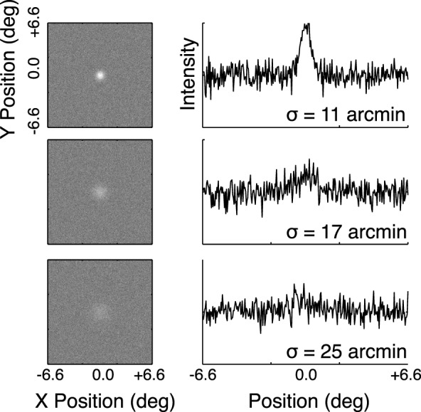
Examples of the stimuli are shown in the left column, and cross-sections (normalized intensity vs. horizontal position) are shown on the right.

The main challenge was to extract a parameter estimate from the tracking task that was analogous to a parameter traditionally used to quantify performance in a psychophysical task. In a traditional 2AFC (two-alternative forced choice) psychophysical experiment for assessing position discrimination, the tools of signal detection theory are used to obtain an estimate of the signal-to-noise ratio along a hypothetical decision axis. With reasonable assumptions, the observation noise associated with position estimates can be determined.

For a tracking experiment, recovering observation noise requires a model of tracking performance that incorporates an estimate of the precision with which a target can be localized. General tracking problems are ubiquitous in engineering and the optimal control theory of simple tracking tasks is well established. For cases like our tracking task, the Bayesian optimal tracker is the Kalman filter (Kalman, 1960). The Kalman filter explicitly incorporates an estimate of the performance-limiting observation noise as a key component. The next few paragraphs provide a brief discussion of the logic behind a Kalman filter. The purpose of the discussion is to make clear how observation noise affects a Kalman filter's tracking performance.

In order to track a target, the Kalman filter uses the current observation of a target's position, information about target dynamics, and the previous estimate of target position to obtain an optimal (i.e., minimum mean square error) estimate of true target position on each time step. Importantly, the previous estimate has a (weighted) history across previous time steps built-in. How these values (the noisy observation, target dynamics, and the previous estimate) are combined is dependent on the relative size of the two sources of variance present in the Kalman filter: (a) the observation noise variance (i.e., the variance associated with the current sensory observation), and (b) the target displacement variance (i.e., the variance driving the target position from time step to time step).

When the observation noise variance is low relative to the target displacement variance (i.e., target visibility is high), the difference between the previous position estimate and the current noisy observation is likely to be due to changes in the position of the target. That is, the observation is likely to provide reliable information about the target position. As a result, the previous estimate will be given little weight compared to the current observation. Tracking performance will be fast and have a short lag.

On the other hand, if observation noise variance is high relative to target displacement variance (i.e., target visibility is low), then the difference between the previous position estimate and the current noisy observation is likely driven by observation noise. In this scenario, little weight will be given to the current observation while greater weight will be placed on the previous estimate. Tracking performance will be slow and have a long lag. As we will see, the Kalman filter qualitatively predicts the data patterns observed in this set of experiments, under the assumption that increasing blob width reduces target visibility, thereby increasing observation noise.

In our analysis, we fit human tracking data with a Kalman filter. We allowed the model's observation noise parameter, R, to vary as a free parameter. The parameter value (observation noise variance) that maximizes the likelihood of the fit under the model is our estimate of the target position uncertainty that limits the tracking performance of the observer.

In the results that follow, we show that using a Kalman filter to model the human tracking data yields essentially the same estimates of position uncertainty as do standard methods in traditional psychophysics. The correlations between the results of the two paradigms are extremely high, with over 97% of the variance accounted for. We also show that more easily computed statistical summaries of tracking data (e.g., the width of the peak of the cross-correlation between stimulus and response) correlate almost as highly with traditional psychophysical results. To summarize, an appropriately constructed tracking task is a fun, natural way to collect large, rich datasets, and yield essentially the same results as traditional psychophysics in a fraction of the time.

General methods

Observers

Three of the authors served as observers (LKC, JDB, and KLB). All had normal or corrected-to-normal vision. Two of the three had extensive prior experience in psychophysical experiments. All the observers participated with informed consent and were treated according the principles set forth in the Declaration of Helsinki of the World Medical Association.

Stimuli

The target was a luminance increment (or “blob”) defined by a two-dimensional Gaussian function embedded in dynamic Gaussian pixel noise. We manipulated the spatial uncertainty of the target by varying the space constant (standard deviation, hereafter referred to as “blob width”) of the Gaussian, keeping the luminous flux (volume under the Gaussian) constant. Examples of these are shown in Figure 1. The space constants were 11, 13, 17, 21, 25, and 29 arcmin; the intensity of the pixel noise was clipped at three standard deviations, and set such that the maximum value of the 11 arcmin Gaussian plus three noise standard deviations corresponded to the maximum output of the monitor. We used this blob target (e.g., as opposed to a Gabor patch) because, for the tracking experiment, we wanted a target with an unambiguous bright center at which to point.

In the tracking experiment, the target moved according to a random (Brownian) walk for 20 s (positions updated at 60 Hz) around a square field of noise about 6.5° (300 pixels) on a side. To specify the walk, we generated two sequences of Gaussian white noise velocities (v_x, v_y) with a one pixel per frame standard deviation. These were summed cumulatively to yield a sequence of x,y pixel positions. Also visible was a 2 × 2 pixel (2.6 arcmin) square red cursor that the observer controlled with the mouse.

Apparatus

The stimuli were displayed on a Sony OLED flat monitor running at 60 Hz. The monitor was gamma-corrected to yield a linear relationship between luminance and pixel value. The maximum, minimum, and mean luminances were 134.1, 1.7, and 67.4 cd/m², respectively.

All experiments were run using custom code written in MATLAB and used the Psychophysics Toolbox (Brainard, 1997; Pelli, 1997; Kleiner, Brainard, Pelli, & Ingling, 2007). A standard USB mouse was used to record the tracking data, and a standard USB keyboard was used to collect the psychophysical response data.

Experiments 1 and 2 (the tracking and main psychophysics experiments) were run using a viewing distance of 50 cm giving 45.5 pixels/° of visual angle. Experiment 3, a supplementary psychophysical experiment on the effect of viewing duration, was run using a viewing distance of 65.3 cm giving 60 pixels/°. In both cases, the observer viewed the stimuli binocularly using a chin cup and forehead rest to maintain head position.

Experiment 1. Tracking

In the tracking experiment, observers tracked a randomly moving Gaussian blob with a small red cursor using a computer mouse. The data were fit with a Kalman filter model of tracking performance. The fitted values of the model parameters provide estimates of the human uncertainty about target position (i.e., observation noise).

Methods

Each tracking trial was initiated by a mouse click. Subjects tried to keep the cursor centered on the target for 20 s while the target moved according to the random walk. The first five seconds of one such trial are shown in Movie 1.

Movie 1.

Download video file ^{(733.8KB, mov)}

DOI: 10.1167/15.3.14.M1

A 5 s example of an experimental trial (actual trials were 20 s long). The luminance blob performed a two-dimensional random walk. Each position was the former position plus normally distributed random offsets (SD = 1 pixel) in each dimension (x,y). The subject was attempting to keep the red cursor centered on the blob.

A block consisted of 10 such trials at a fixed blob width. Subjects ran one such block at each of the six blob widths in a single session. Each subject ran two sessions and within a session, block order (i.e., blob width) was randomized. Thus, each subject completed 20 tracking trials at each blob width, for a total of 24,000 samples (400 s at 60 Hz) of tracking data per blob width. As we later show, this is more data than required to produce reliable results (see Appendix A for an analysis of the precision of tracking estimates vs. sample size). However, we wanted large sample sizes so that we could compare the data with traditional psychophysics with high confidence.

Results

The tracking task yields time series data: the two-dimensional spatial position of a target (left panel of Figure 2; black curve) and the position of the tracking cursor (red curve). The remaining panels in Figure 2 show the horizontal and vertical components of the time series data in the left panel as a function of time. Subjects were able to track the target. The differences between the two time series (true and tracked target position), and how these differences changed with target visibility (blob width), constitute the dependent variable in the tracking experiment.

Figure 2.

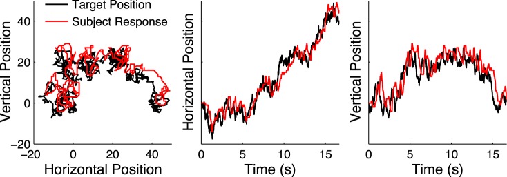
Target position and subject response for a single tracking trial (left plot). The middle and right plots show the corresponding time series or the horizontal and vertical positions, respectively.

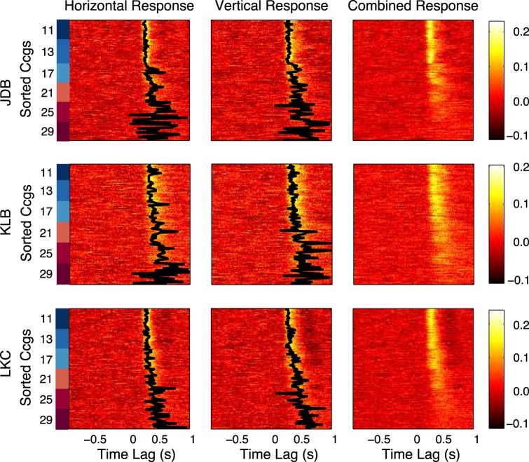
A common tool for quantifying the relationship between target and response time series is the cross-correlogram (CCG; see e.g., Mulligan, Stevenson, & Cormack, 2013). A CCG is a plot of the correlation between two vectors of time series data as a function of the lag between them. Figure 3 shows the cross-correlation as a function of lag for each individual tracking trial sorted by blob width (i.e., target visibility). Each panel shows CCGs per trial in the form of a heat map (low to high correlation mapped from red to yellow) sorted on the y axis by blob width during the trial. Each row of panels is an individual subject. Because our tracking task has two spatial dimensions, each trial yields a time series for both the horizontal and vertical directions. The first and second columns in the figure show the horizontal and vertical CCGs, respectively, and the black line traces the maximum value of the CCGs across trials. As blob width increases (i.e., lower peak signal-to-noise), the response lag increases, the peak correlation decreases, and the location of the peak correlation becomes more variable. As there were no significant differences between horizontal and vertical tracking in this experiment, the rightmost column of Figure 3 shows the average of the horizontal and vertical responses. Clearly, the tracking gets slower and less precise as the blob width increases (i.e., target visibility decreases).

Figure 3.

Heatmaps of the cross-correlations between the stimulus and response velocities. Left and Middle columns show horizontal and vertical response components, respectively. Each row of a subpanel represents an individual tracking trial, and the trials have been sorted by target blob width (measured in arcmin and labeled by color blocks that correspond with the curve colors in Figure 4); beginning with the most visible stimuli at the tops of each subpanel. The black lines trace the peaks of the CCGs. The right column shows the average of horizontal and vertical response correlations within a trial (i.e., average of left and middle columns).

Figure 4 shows a plot of the average CCG across trials for each blob width for each of the three subjects (a replot of the data from Figure 3, collapsing across trial within each blob width). The CCGs sort by blob width: as blob width increases, the height of the CCG peak decreases, the lag of the CCG peak increases, and the width of the CCG increases. These results show that tracking performance decreases monotonically with the signal-to-noise ratio. This result is consistent with the expected result in a traditional psychophysical experiment. That is, as target visibility decreases, the observer's ability to localize a target should also decrease.

Figure 4.

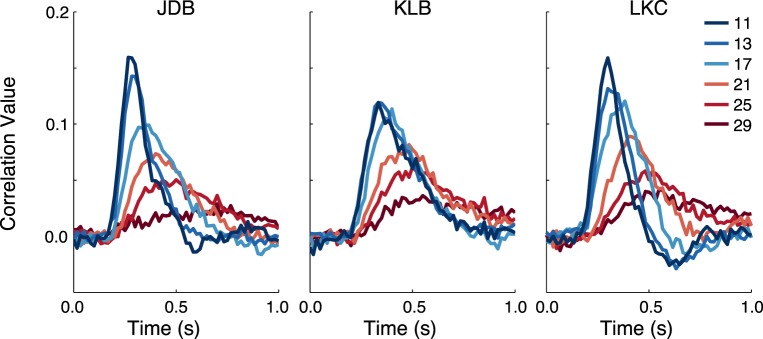
Average CCGs for blob width (curve color, identified in the legend by their σ in arcmin) for each of the three observers (panel). The peak height, location of peak, and width of curve (however measured) all sort neatly by blob width, with the more visible targets yielding higher, prompter, and sharper curves. This shows that there is at least a qualitative agreement between measures of tracking performance and what would be expected from a traditional psychophysical experiment.

In order to quantify tracking performance in a way that can be directly related to traditional psychophysics, we fit a Kalman filter model to the data and extracted the observation noise variance (filter parameter R) as a measure of performance. Figure 5 illustrates the details of the Kalman filter in the context of the tracking task. Our experiment generated two position values at each time step in a trial: (a) the true target position (x_t) on the screen, and (b) the position of the observer's cursor (x̂_t), which was his or her estimate of the target position (plus dynamics due to arm kinematics, motor noise, and noise introduced by spatiotemporal response properties of the input device). The remaining unknowns in the model are the noisy sensory observations, which are internal to the observer and cannot be measured directly. These noisy sensory observations are modulated by a single parameter; the observation noise variance (R). We fit the observation noise variance (R) of a Kalman filter model (per subject) by maximizing the likelihood of the human data under the model given the true target positions (see Appendix B for details). Note that we have assumed for the purpose of this analysis that the aforementioned contributions of arm kinematics, motor noise, and input device can be described by a temporal filter with fixed properties.

Figure 5.

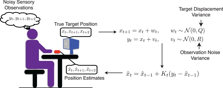
Illustration of the Kalman filter and our experiment. The true target positions and the estimates (cursor positions) are known, while the sensory observations, internal to the observer, are unknown. We estimated the variance associated with the latter, denoted by R, by maximizing the likelihood of the position estimates given the true target positions by adjusting R as a free parameter.

For a given observer, this maximum-likelihood fitting procedure was done simultaneously across all the runs for a given blob width throwing out the first second of each run. This yielded one estimate of R for each combination of observer and blob width. Error distributions on R were computed via bootstrapping (i.e., resampling was performed on observers' data by resampling whole trials).

This approach is different from traditional Kalman filter applications. Typically, the Kalman filter is used in situations when the noisy observations are known. The filter parameters (Q and R) are estimated and then the filter can be used to generate estimates (x̂_t) of the true target positions (x_t). In our case, the noisy observations cannot be observed and we estimate the observation noise variance (filter parameter R) given the true target positions (x_t), the target position estimates (x̂_t), and the target displacement variance (filter parameter Q). Thus, we essentially use the Kalman filter model in reverse, treating x_t and x̂_t as known instead of y_t, in order to accomplish the goal of estimating R.

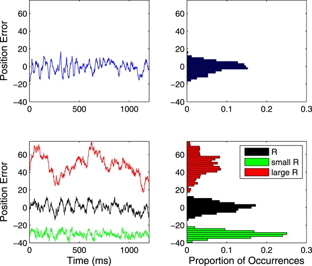
We attempt to convey an intuition about what the fitting accomplishes in Figure 6. The top-left panel shows an example trace of subject position error (i.e., subject response minus target location). This position error reflects observation noise (and presumably some motor noise and apparatus noise). The bottom-left panel shows three possible traces of position error generated by simulating from the model—the black trace using an approximately correct value of R (such as that on which our analysis converges), and two others (offset vertically for clarity) using incorrect values. Note that, visually, the standard deviations of the red and green traces are too large and too small, respectively. However, the standard deviation of the black curve is approximately equal to the standard deviation of the blue curve (the human error trace). This point is made clearer by examining the distributions of these residual position values collapsed across time (right column). Note that the black distribution has roughly the same width as the blue distribution, while the others are too big or too small. This is essentially what our fitting accomplishes: finding the Kalman filter parameter, R, that results in a distribution of errors with a standard deviation that is “just right.” (Brett, 1987).

Figure 6.

The left column shows the positional errors (response position−target position) over time of a subject's response (top) and three model responses (bottom, offset vertically for clarity); the black position error trace results from a roughly correct estimate of R. The right column shows the histograms of the positions from the first column. The distribution from the model output with the correct noise estimate (black), has roughly the same width as that from the human response (blue, top).

The results of this analysis are shown in Figure 7, which plots the square root of the estimated observation noise variance, , as a function of blob width for each of the three observers. The estimate of represents an observer's uncertainty about the target location. For the remainder of the paper we refer to as the positional uncertainty estimate. The results are systematic, with the tracking noise estimate increasing as a function of blob width in the same way for all three observers. The results are intuitive, in that, as the width of the Gaussian blob increases, the precision with which an observer can estimate the target position decreases, yielding greater error in pointing to the target with a mouse. Qualitatively, they are similar to what we would expect to see in a plot of threshold versus signal-to-noise ratio derived from traditional psychophysical methods.

Figure 7.

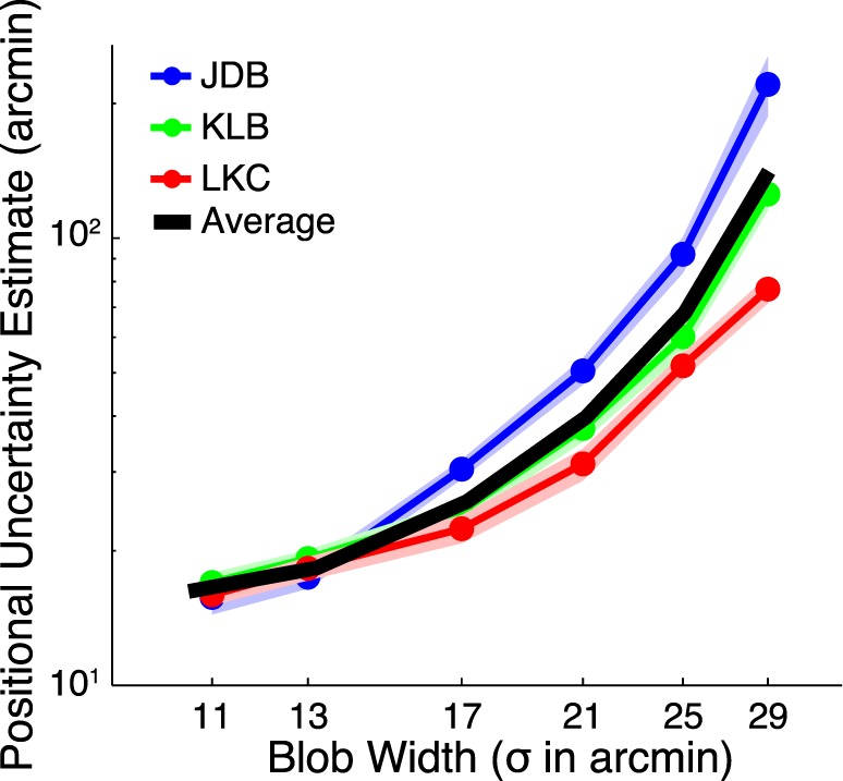
Positional uncertainty estimate from the Kalman filter analysis plotted as a function of the Gaussian blob width for three observers. Both axes are logarithmic. The pale colored regions indicate ±SEM computed by bootstrapping. The black line is the mean across the observers.

Discussion

We used a Kalman filter to model performance in a continuous tracking task. The values of the best fitting model parameters provide estimates of the uncertainty with which observers localize the target. The results were systematic and agree qualitatively with the cross-correlation analysis, which is a more conventional way to analyze time-series data. Next, we determine the quantitative relationship between estimates of positional uncertainty obtained from tracking and from a traditional psychophysical experiment.

Experiment 2. Forced-choice position discrimination

In this experiment, observers attempted to judge the direction of offset of the same luminance targets used in the previous experiment. The results were analyzed using standard methods to estimate the (horizontal) positional uncertainty that observers had about target position.

Forced-choice methods

The apparatus was as described in General methods. An individual trial is depicted in Figure 8. On each video frame throughout a trial, a new sample of Gaussian distributed noise, independent in space and time (e.g., white), was added to the target. The noise parameters were identical to those used in the tracking experiment. On each trial, the observer saw two 250 ms target presentations, separated by a 100 ms interstimulus interval. In one interval, the target always appeared in the center of the viewing area. In the other interval, the target appeared at one of nine possible stimulus locations (four to the left, four to the right, and zero offset). The observer's task was to indicate whether the second interval target was presented to the left or right of the first interval target. Data were collected in blocks of 270 trials. Blob width was fixed within a block. Targets were presented 30 times at each of the nine comparison locations in a pseudorandom order. Each observer completed three blocks for each of the six target blobs, for a total of 4,860 trials per observer (270 trials/block × 3 blocks/target × 6 targets/observer).

Figure 8.

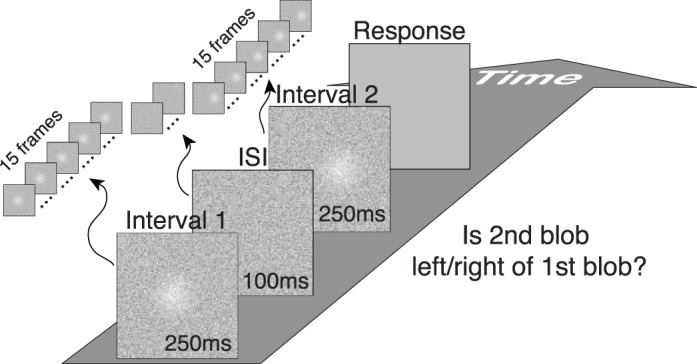
Timeline of a single trial. The task is a two interval forced-choice task. The stimuli were Gaussian blobs in a field of white Gaussian noise. Subjects were asked to indicate whether the second blob was presented to the left or right of the first blob.

The data for each run were fit with a cumulative normal psychometric function (ϕ), and the spatial offset of the blob corresponding to d′ = 1.0 point (single interval) was interpolated from the fit. The d′ for single interval was used because it corresponds directly to the width of the signal + noise (or noise alone) distribution. Because P_R = ϕ ( /2) = ϕ ( / ) where P_R is the percent rightward choices and d′_2I is the 2-interval d′, threshold was defined as the change in position necessary to travel from the 50% to the 76% rightward point on the psychometric function.

Results

Thresholds as a function of blob width are shown in Figure 9. The solid data points are the threshold estimates from fitting all of an observer's data at a given blob width, and the error bands are ± one standard error obtained by bootstrapping from the raw response data. The heavy black line shows the (arithmetic) mean for the three observers. The thresholds for all observers increase with increasing blob width, with a hint of a lower asymptote for the smallest targets. This is the same basic pattern of data we would expect using an equivalent noise paradigm in a detection (e.g., Pelli, 1990) or localization task, as the amount of effective external noise increases with increasing blob width.

Figure 9.

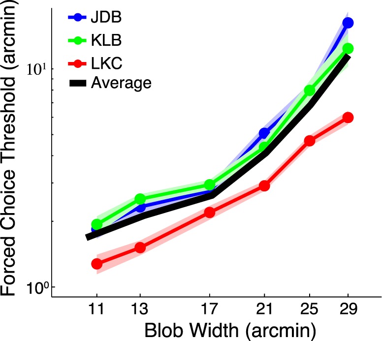
Forced-choice threshold as a function of blob width. Each subject's average data are shown by the solid points, and the bands indicate bootstrapped SEM. Both axes are logarithmic. The solid black line shows the average across subjects.

Discussion

The thresholds presented in Figure 9 correspond to a d′ of 1.0, thus representing the situation in which the relevant distributions along some decision axis were separated by their common standard deviation. Assuming that the position of the target distribution on the decision axis is roughly a linear transformation of the target's position in space, then this also corresponds to the point at which the targets were separated by roughly one standard deviation of the observer's uncertainty about their position. Thus, the offset thresholds serve as an estimate of the width of the distribution that describes the observer's uncertainty about the target's position. This is exactly what the positional uncertainty estimates represented in the tracking experiment. In fact, it would be reasonable to call the forced-choice thresholds “positional uncertainty estimates” instead. The use of the word threshold is simply a matter of convention in traditional psychophysics.

Figure 10 shows a scatterplot of the results from the tracking experiment (y coordinates) versus those from the traditional psychophysics (x coordinates). The log-log slopes are 0.98 (LKC), 1.12 (JDB), and 1.02 (KLB). The corresponding correlations are 0.985, 0.996, and 0.980, respectively. Obviously, the results are in good agreement; the change in psychophysical thresholds with blob width is accounting for over 96% of the variance in the estimates obtained from the tracking paradigm, the high correlation indicates that the two variables are related by an affine transformation. In our case (see Figure 10), the variables are related by a single scalar multiplier. This suggests to us that the same basic quantity is being measured in both experiments.

Figure 10.

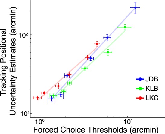
Scatter plot of the position uncertainty estimated from the tracking experiment (y axis) as a function of the thresholds from traditional psychophysics (x axis) for our three observers. The log-log slope is very close to 1 and the percentage of variance accounted for is over 96% for each observer.

There is, however, an offset of about one log unit between the estimates generated by the two experiments. For example if, for a given blob width, the 2AFC task yields an estimate of 1 arcmin of positional uncertainty, the tracking task would yield a corresponding estimate of 10 arcmin. The relative estimates are tightly coupled, but we would like to understand the reasons for the discrepancy in the absolute values. One obvious candidate is temporal integration, which would almost certainly improve performance in the psychophysical task relative to the tracking task.

Experiment 3. Temporal integration

One possible reason for the fixed discrepancy between the positional uncertainty estimates in the tracking task and the thresholds in the traditional psychophysical task is temporal integration. In the traditional task, the observers could benefit by integrating information across multiple stimulus frames (up to 15 per interval) in order to do the task. If subjects integrated perfectly over all 15 frames, threshold would be times lower than the thresholds that would be estimated from 1 frame. The positional uncertainty estimated in the tracking task is the positional uncertainty associated with a single frame. Thus, it is possible that approximately half of the discrepancy between the forced-choice and tracking estimates of positional uncertainty is due to temporal integration in the forced-choice experiment.

It's also important to consider how the tracking task may be affected by temporal integration. In practice, if an observer's sensory–perceptual system is performing temporal integration then they are responding to a spatially smeared representation of the moving—a motion streak—instead of the instantaneous stimulus. Temporal integration per se is not modeled in our implementation of the Kalman filter, but its presence in the data would result in an overestimate of observation noise. This effect of temporal integration might further add to the discrepancy between the measurements of positional uncertainty.

In this experiment, we sought to measure our observers' effective integration time and the degree to which this affected the psychophysical estimates of spatial uncertainty.

Methods

The methods for this experiment were the same as for Experiment 2 (above), except that the duration of the stimulus intervals was varied between 16.7 ms (one frame) and 250 ms (15 frames) while blob width was fixed. The interstimulus interval remained at 100 ms. Observers KLB and JDB ran at a 17-arcmin blob width, and LKC ran at 21 arcmin (values that yielded nearly identical thresholds for the three observers in Experiment 2). These were run using the same Sony OLED monitor, but driven with a Mac Pro at a slightly different viewing distance (see General methods).

Results

Figure 11 shows the offset thresholds as a function of stimulus duration. As in Figure 9, the data points are the interpolated thresholds (d′ = 1) from the cumulative normal fits, the error bands show ±1 standard error estimated by bootstrapping, and the solid black line show the mean thresholds across subject. Thresholds for all observers decreased with increased stimulus duration at the expected slope of 1/ (dashed line for reference) until flattening out at roughly 50 to 100 ms, or three to five frames (Watson, 1979; Nachmias, 1981).

Figure 11.

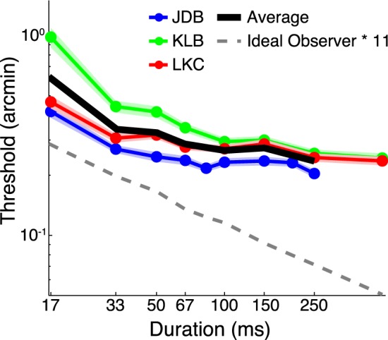
Threshold as a function of stimulus duration. Each subject's average data are shown by the solid points. Both axes are logarithmic. Data points and error bands are as in Figure 9. The gray line displays the performance of an ideal observer shifted up by a factor of 11.

Discussion

The thresholds at single frame durations approximate what thresholds would be if observers could not benefit from temporal integration in the psychophysical task. As we argued earlier, moreover, the tracking task could not have benefited from temporal integration; if anything, using multiple frames would cause the uncertainty estimates from the tracking task to be too high. It would therefore be conservative to correct the psychophysical thresholds from Experiment 2 upward by a factor corresponding to the ratio between the single frame and 15 frame thresholds from Experiment 3. This turns out to be about a factor of 2, and would reduce the absolute difference between the tracking and psychophysical estimates from a factor of 10 to about a factor of 5.

An important next step in understanding temporal integration is to perform a comparable experiment in the tracking task (i.e., manipulating the rate at which the stimulus moves). Such a follow-up study would will further clarify the relationship between the forced-choice task and the tracking task, as well as solidify the appropriate stimulus for a psychophysics tracking task.

General discussion

In this paper, we have shown that data from a simple tracking task can be analyzed in a principled way that yields essentially the same answers that result from a traditional psychophysical experiment using comparable stimuli in a fraction of the time. In this analysis, we modeled the human observer as a dynamic system controller—specifically a Kalman filter. The Kalman filter is typically used to produce a series of estimated target positions given an estimate of the observation noise (e.g., known from sensor calibration). We, in contrast, used the Kalman filter to estimate the observation noise given a series of estimated target positions generated by observer during our experiments.

The conceptualization of a human as an element of a control system in a tracking task is not a novel concept. In fact, this seems to be one of the problems that Kenneth Craik was working on at the time of his death—two of his manuscripts on the topic were published posthumously by the British Journal of Psychology (Craik, 1947, 1948). Because circuits or, later, computers, are generally much better feedback controllers than humans, there has been less interest in the specifications of human-as-controller with a few exceptions: studies of pilot performance in aviation, motor control, and eye movement research (in some ways a subbranch of motor control, in other ways a subbranch of vision).

It is clear that the job of a pilot, particularly when flying with instruments, is largely to be a dynamic controller that minimizes the error between an actual state and a goal state. For example, the goal state might be a particular altitude and heading assigned by air traffic control. The corresponding actual state would be the current heading and altitude of the airplane. The error to be minimized is the difference between the current and goal states as represented on the aircraft's instruments. It comes as no surprise, then, that a large literature has emerged in which the pilot is treated as, in Craik's terms, an engineering system that is itself an element within a larger control system. However the pilot's sensory systems are not generally considered a limiting factor; pilot errors are never due to poor acuity (to our knowledge) but rather due to attentional factors related to multitasking or, occasionally, sensory conflict (visual vs. vestibular) resulting in vertigo. As such, while tracking tasks are often studied in the aviation literature, is not done to assess a pilots' sensory (or basic motor) capabilities.

The motor control literature involving tracking tasks can be divided into three main branches: eye movement control (e.g., Mulligan et al., 2013), manual (arm and hand) control (e.g., Wolpert & Ghahramani, 1995; Berniker & Kording, 2008), and, to a lesser extent, investigations of the interaction between the two (e.g., Brueggemann, 2007; Burge, Ernst, & Banks, 2008; Burge, Girshick, & Banks, 2010; van Dam & Ernst, 2013). Within the motor control literature, there are several examples of the use of the Kalman filter to model a subject's tracking performance. Some of these focus almost exclusively on modeling the tracking error as arising from the physics of the arm and sensorimotor integration (Wolpert & Ghahramani, 1995; Berniker & Kording, 2008). Others provide a stronger foundation for our work by demonstrating how changing the visual characteristics of a stimulus affects human performance in a manner that can be reproduced by manipulating parameters of the Kalman filter (Burge et al., 2008). Taken together, this body of literature provides strong support for the idea that the human ability to adapt to and track a moving stimulus is consistent with the performance of a Kalman filter. We extend this literature by using the Kalman filter to explicitly estimate visual sensitivity.

In the results section, we showed a strong empirical relationship between the data from tracking and forced-choice tasks. To further this comparison, it would be useful to know what optimal (ideal observer) performance would be. Obviously, if ideal performance in the two tasks were different, then we wouldn't expect our data from Experiments 1 and 2 to be identical, even if the experiments were effectively measuring the same thing. In other words, if the two experiments yielded the same efficiencies, then we would know they were measuring exactly the same thing. Of course, this unrealizable in practice because the tracking response necessarily comprises motor noise (broadly defined) in addition to sensory noise, whereas the motor noise is absent in forced-choice psychophysics due to the crude binning of the response. What we can realistically expect is to see efficiencies from tracking and forced-choice experiments that are highly correlated but with a fixed absolute offset reflecting (presumably) motor noise and possibly other factors.

The ideal observer for the forced-choice task is based on signal detection theory (e.g., Green & Swets, 1966; Geisler, 1989; Ackermann & Landy, 2010). To approximate the ideal observer in a computationally efficient way, we used a family of templates identical to the target but shifted in spatial location to each of the possible stimulus locations. These were multiplied with the stimulus (after averaging across the 15 frames in each interval). The model observer chose the direction that corresponded to the maximum template response, defined as the product of the stimulus with the template (in the case of the zero offset template, then the model observer guessed with p(right) = 0.5). The stimuli and templates were rearranged as vectors so that the entire operation could be done as a single dot product as in Ackermann and Landy (2010). The ideal observer was run in exactly the same experiment as the human observers, except that the offsets were a factor of 10 smaller, which was necessary to generate good psychometric functions because of the model's greater sensitivity.

The left panel of Figure 12 shows the ideal observer's threshold as a function of blob width (black line), along with the human observers' data from Figure 7. The gray line shows the ideal thresholds shifted upward by a factor of 20. The results are as expected: the humans are overall much less sensitive than ideal, they approach a minimum threshold on the left, increase with roughly the same slope as the ideal in the middle, and then begin (or would begin) to accelerate upward as the target becomes invisible. A maximum efficiency of about 0.25% (a 1 : 20 ratio of human to ideal d′) is approached at middling blob widths, which is consistent with previous work using grating patches embedded in noise (Simpson, Falkenberg, & Manahilov, 2003).

Figure 12.

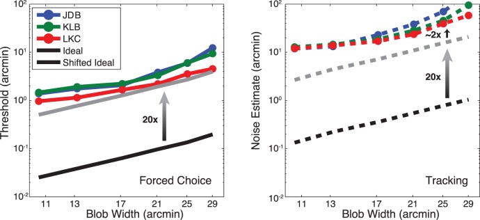
Relationship between human observers and an ideal observer. Forced-choice human threshold estimates (left) and tracking noise estimates (right) are replotted (blue, green, and red lines). The ideal observers are depicted in black and the shifted ideal in gray.

In the tracking task, the ideal observer's goal was to estimate the location of the stimulus on each stimulus frame. To implement this, a set of templates identical to the stimulus but varying in offset in one dimension around the true stimulus location was multiplied with the stimulus each frame. The position estimate for each frame was then the location of the template producing the maximum response. The precision with which this observer could localize the target was simply the standard deviation of the position estimates relative to the true target location (i.e., the standard deviation of the error). Note that as the ideal observer had no motor system to add noise, this estimate corresponds specifically to the measurement noise in the Kalman filter formulation. It also corresponds to the ideal observer for a single-interval forced-choice task observer given only one stimulus frame per judgment.

The right panel of Figure 12 shows the ideal observer's estimated sensory noise (dashed black line) as a function of blob width, along with the corresponding estimates of spatial uncertainty based on the Kalman filter fit to the human data replotted from Figure 12. The slope is the same as for the forced-choice task. The dashed gray line is the ideal threshold line shifted upward by a factor of 20 (the same amount as the shift in the left panel). After a shift reflecting efficiency in the forced-choice task, there is roughly a factor of 2 difference remaining. As previously mentioned, this is not surprising because the observer's motor system must contribute noise to the tracking task but not in the forced-choice task.

We have constructed a principled observer model for the tracking task that yields comparable results to traditional forced-choice psychophysics, establishing the validity of the tracking task for taking psychophysical measurements. Here, we introduce simpler methods of analysis for the tracking task that provide an equivalent measure of performance. We show that the results from an analysis of the CCGs (introduced earlier) are just as systematically related to the forced-choice results as are those from the Kalman filter observer model.

The left panel of Figure 13 shows CCGs (data points) for observer LKC (replotted from Figure 4, right), along with the best fitting sum-of-Gaussians. Although Gaussians are not theoretically good models for impulse response functions, we used them as an example for their familiarity and simplicity. Based on visual inspection they seem to provide a rather good empirical fit to the data. We used a sum of two Gaussians (the second one lagged and inverted), rather than a single Gaussian, in order to model the negative (transient) overshoot seen in the data from the three smallest blob widths for LKC and the smallest blob width for JDB. For all other cases, the best fit resulted in a zero (or very near zero) amplitude for the second Gaussian.

Figure 13.

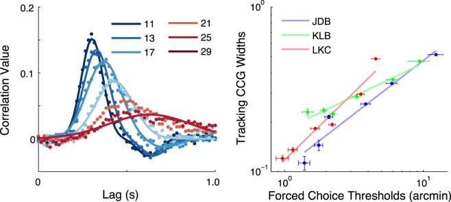
The left panel depicts the CCGs for subject LKC sorted by blob width (identified in the legend by their σ in arcmin). The right panel shows the forced-choice estimates versus the CCG widths (of the positive-going Gaussians) from the tracking data. Error bars correspond to SEM.

The right panel of Figure 14 shows the standard deviations of the best fit positive Gaussians from the left panel plotted as a function of the corresponding forced-choice threshold estimates. As with the Kalman filter estimates, the agreement is very good indicating that the tracking data yield basically the same answer as the forced-choice data regardless of analysis.

Figure 14.

Parameters (amplitude, lag, and width) are very highly correlated. From the left to right, the panels represent: lag versus amplitude, width versus lag, and amplitude versus width. The correlation coefficients that correspond to each of these relationships are inset in each panel. These parameters are calculated from observer LKC's data.

Two further points can be made about the simple Gaussian fits to the CCGs. First, the best-fit values for the three parameters (amplitude, lag or mean, and standard deviation) are very highly correlated with one another despite being independent in principle. The best-fit parameter values plotted against one another pairwise are shown in Figure 14. The relationships are plotted (from left to right) for amplitude versus lag, lag versus width, and width versus amplitude; the corresponding correlation coefficients are shown as insets. Clearly, it would not matter which parameter was chosen as the index of performance. As an aside, including the second Gaussian (negative) in fitting the CCG is unnecessary. The results are essentially identical when only a single positive Gaussian is used fit to the CCGs.

In conclusion, we have presented a simple dynamic tracking task and a corresponding analysis that produce estimates of observer performance or, more specifically, estimates of the uncertainty limiting observers' performance. These estimates correspond quite closely with the estimates obtained from a traditional forced-choice psychophysical task done using the same targets. Compared with forced-choice stimuli, this task is easy to explain, intuitive to do for naive observers, and fun. Informally, we have run children as young as 5 years old on a more game-like version of the task, and all were very engaged and requested multiple “turns” at the computer. We find it likely that this would apply more generally, not only to children, but also to many other populations that have trouble producing large amounts of psychophysical data. Finally, the “tracking” need not be purely spatial; one could imagine tasks in which, for example, the contrast of one target was varied in a Gaussian random walk, and the observers' task was to use a mouse or a knob to continuously match the contrast of a second target to it. In conclusion, the basic tracking paradigm presented here produces rich, informative data sets that can be used as fast fun windows onto observers' sensitivity.

Appendix A. Convergence of Kalman filter uncertainty estimate

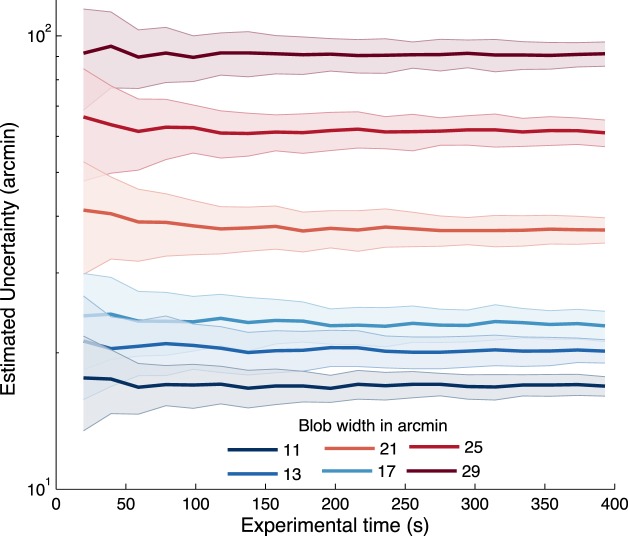
Figure A1 demonstrates the time course of the convergence of the Kalman filter uncertainty estimate on one subject's tracking data. Each of the solid lines represents the average estimated uncertainty ( ) for a particular stimulus width produced by performing bootstrapping on the fitting procedure as we increase the total experimental time used to estimate R. The clouds around these estimates represent the standard error. It requires relatively little experimental time to produce reliable estimates of uncertainty using our Kalman filter fitting procedure. Note that the estimates for the four most difficult targets are easily discriminable in under two minutes of data collection per target condition.

Figure A1.

Estimated uncertainty ( ) versus experimental time used to estimate R. Error bounds show ±SEM. Blob width is indicated by curve color and identified in the legend by its σ in arcmin.

Appendix B. Kalman filter for maximum-likelihood fitting procedure

In this work we use a Kalman filter framework to estimate subjects' observation noise variance (R, see Figure 5) and therefore also position uncertainty, which is defined as . The two time series produced by the experimental tracking paradigm—target position (x_t) and subject response (x̂_t)—are used in conjunction with the Kalman filter in order to fit observation noise variance by maximizing p(x̂|x), the probability of the position estimates given the target position under the Kalman filter model.

Consider the tracking paradigm a simple linear dynamical system with no dynamics or measurement matrices:

where the x_t represents the target position, and y_t represents the subjects' noisy sensory observations, which we cannot access directly (see Figure 5).

Given a set of observations y_1:t and the parameters {Q, R}, the Kalman filter gives a recursive expression for the mean and variance of x_t|y_1:t, that is, the posterior over x at time step t given all the observations y₁, … ,y_t. The posterior is of course Gaussian, described by mean x̂_t and variance P_t. The following set of equations perform the dynamic updates of the Kalman filter and result in target position estimates (x̂_t).

We use this definition (Equations B1 and B2) and the Kalman filter equations (Equations B3–B6) to write p(x̂|x). First, we find the asymptotic value of P_t and then use that to simplify and rewrite the Kalman filter equations in matrix form.

Since Q and R are not changing over time, the asymptotic value of the posterior variance P_t as t → ∞ can be calculated by solving P = (P + Q)R/(P + Q + R) for P, which yields:

In order to further simplify, we will assume P₀ = P_∞; that is, the initial posterior variance will approach some asymptotic posterior variance. A Kalman filter asymptotes in relatively few time steps. In practice, our observers seem to as well, but to be safe we omitted the first second of tracking for each trial to insure that the observers' tracking had reached a steady state. Then the prior variance S, Kalman gain K, and posterior variance P are constant. Thus, the dynamics above can be simplified to:

where K depends only on R:

This makes x̂ a simple auto-regressively filtered version of y. The dynamics can be expressed in matrix form:

where D is a bidiagonal matrix with 1 on the main diagonal and K − 1 on the below-diagonal:

By substituting for y and multiplying by D⁻¹, this can be rewritten as:

Equation B13 in conjunction with Equation B10 gives the expression relating the two time series x̂ and x, to the unknown R. We can use this to write p(x̂|x):

The log likelihood, log(p(x̂|x)) (below), is used in order to perform the maximum-likelihood estimation of R.

where n is the total number of time points (i.e., the length of x and x̂; Note: coefficients D and K are defined in terms of Q and R). The log likelihood for a particular blob width (σ = s) for a given subject is evaluated by taking the sum over all trials with σ = s of p(x̂|x). In our analysis, maximum-likelihood estimation of R is performed for each blob width in order to investigate how the observer's positional uncertainty ( ) changes with increasing blob width (decreasing visibility).

References

- Ackermann J. F., Landy M. S. (2010). Suboptimal choice of saccade endpoint in search with unequal payoffs. Journal of Vision , 10 (7): 14, http://www.journalofvision.org/content/10/7/530, doi:10.1167/10.7.530. [Abstract] [Google Scholar]
- Berniker M., Kording K. (2008). Estimating the sources of motor errors for adaptation and generalization. Nature Neuroscience , 11 (12), 1454– 1461. [DOI] [PMC free article] [PubMed] [Google Scholar]
- Brainard D. H. (1997). The psychophysics toolbox. Spatial Vision , 10, 433– 436. [PubMed] [Google Scholar]
- Brett J. (1987). Goldilocks and the three bears (Retold and illustrated). New York: Dodd Mead. [Google Scholar]
- Brueggemann J. (2007). The hand is NOT quicker than the eye. Journal of Vision , 7 (15): 14, http://www.journalofvision.org/content/7/15/54, doi:10.1167/7.15.54. (Note: Actual authors were J. Brueggerman and S. Stevenson, but the latter was omitted from the published abstract by mistake.) [Google Scholar]
- Burge J., Ernst M. O., Banks M. S. (2008). The statistical determinants of adaptation rate in human reaching. Journal of Vision , 8 (4): 14 1– 19, http://www.journalofvision.org/content/8/4/20, doi:10.1167/8.4.20. [Abstract] [DOI] [PMC free article] [PubMed] [Google Scholar]
- Burge J., Girshick A. R.& Banks, M. S. (2010). Visual-haptic adaptation is determined by relative reliability. The Journal of Neuroscience , 30 (22), 7714– 7721. [DOI] [PMC free article] [PubMed] [Google Scholar]
- Craik K. J. W. (1947). Theory of the human operator in control systems: The operator as an engineering system. The British Journal of Psychology , 38 (Pt. 2), 56– 61. [DOI] [PubMed] [Google Scholar]
- Craik K. J. W. (1948). Theory of the human operator in control systems: Man as an element in a control system. The British Journal of Psychology , 38 (Pt. 3), 142– 148. [DOI] [PubMed] [Google Scholar]
- Fechner G. T. (1860). Elemente der psychophysik. Leipzig, Germany: Breitkopf und Härtel. [Google Scholar]
- Geisler W. S. (1989). Sequential ideal-observer analysis of visual discriminations. Psychological Review , 96 (2), 267– 314. [DOI] [PubMed] [Google Scholar]
- Green D. M., Swets J. A. (1966). Signal detection theory and psychophysics. New York: Wiley. [Google Scholar]
- Kalman R. E. (1960). A new approach to linear filtering and prediction problems. Journal of Fluids Engineering , 82 (1), 35– 45. [Google Scholar]
- Kleiner M., Brainard D., Pelli D., Ingling A. (2007). What's new in Psychtoolbox-3. Perception , 36, 14. [Google Scholar]
- Mulligan J. B., Stevenson S. B., Cormack L. K. (2013). Reflexive and voluntary control of smooth eye movements. In Rogowitz B. E., Pappas T. N., de Ridder H. (Eds.), Proceedings of SPIE, Human Vision and Electronic Imaging XVIII: Vol. 8651 (pp 1– 22). [Google Scholar]
- Nachmias J. (1981). On the psychometric function for contrast detection. Vision Research , 21 (2), 215– 223. [DOI] [PubMed] [Google Scholar]
- Pelli D. G. (1990). The quantum efficiency of vision. In Blakemore C. (Ed.), Vision: Coding and efficiency (pp 3– 24) Cambridge, UK: Cambridge University Press. [Google Scholar]
- Pelli D. G. (1997). The VideoToolbox software for visual psychophysics: Transforming numbers into movies. Spatial Vision , 10 (4), 437– 442. [PubMed] [Google Scholar]
- Simpson W. A., Falkenberg H. K., Manahilov V. (2003). Sampling efficiency and internal noise for motion detection, discrimination, and summation. Vision Research , 43 (20), 2125– 2132. [DOI] [PubMed] [Google Scholar]
- van Dam L. C. J., Ernst M. O. (2013). Knowing each random error of our ways, but hardly correcting for it: An instance of optimal performance. PLoS ONE , 8 (10), e78757. [DOI] [PMC free article] [PubMed] [Google Scholar]
- Watson A. B. (1979). Probability summation over time. Vision Research , 19 (5), 515– 522. [DOI] [PubMed] [Google Scholar]
- Wolpert D. M., Ghahramani Z. (1995). An internal model for sensorimotor integration. Science , 269, 1880– 1883. [DOI] [PubMed] [Google Scholar]