Estimating the Burden of Recurrent Events in the Presence of Competing Risks: The Method of Mean Cumulative Count

Abstract

Cumulative incidence has been widely used to estimate the cumulative probability of developing an event of interest by a given time, in the presence of competing risks. When it is of interest to measure the total burden of recurrent events in a population, however, the cumulative incidence method is not appropriate because it considers only the first occurrence of the event of interest for each individual in the analysis: Subsequent occurrences are not included. Here, we discuss a straightforward and intuitive method termed “mean cumulative count,” which reflects a summarization of all events that occur in the population by a given time, not just the first event for each subject. We explore the mathematical relationship between mean cumulative count and cumulative incidence. Detailed calculation of mean cumulative count is described by using a simple hypothetical example, and the computation code with an illustrative example is provided. Using follow-up data from January 1975 to August 2009 collected in the Childhood Cancer Survivor Study, we show applications of mean cumulative count and cumulative incidence for the outcome of subsequent neoplasms to demonstrate different but complementary information obtained from the 2 approaches and the specific utility of the former.

In many clinical studies, it is of interest to estimate the cumulative probability of developing an event by a given time. The complement of a Kaplan-Meier (KM) product limit estimate has been widely used to estimate this cumulative probability. However, when there are competing-risk events, which are events that either preclude the occurrence of the event of interest or fundamentally alter its probability of occurrence (1), the method of cumulative incidence (CumI) should be used. The KM method is not appropriate when competing-risk events are present, because it does not distinguish competing-risk events from censoring, which can result in inflated cumulative probability estimates. The CumI method properly removes individuals who had a competing-risk event from the risk set for the event of interest.

The CumI approach estimates the cumulative probability of the first event of interest over time: Subsequent occurrences of the event of interest are not included. When examining the probability of event occurrence within subpopulations of subjects defined by different treatments or other risk factors (i.e., etiological inference), it may be sensible for the analysis to consider only the first occurrence of the event in each subject, particularly if the occurrence of the first event changes the underlying risk and/or biology of the subsequent event (e.g., by treatment).

However, in many studies, the outcome variable of interest is a recurrent event: Each individual in the study may experience the event of interest multiple times over the study period (2). For example, survivors of childhood cancer are at risk of subsequent neoplasms, which can reoccur (3, 4). With the CumI method, survivors who experience recurrent subsequent neoplasms are treated in the analysis the same way as those who experience only 1 subsequent neoplasm, thus underestimating the total burden of subsequent neoplasms in this study population. Other examples of such outcomes include hospitalizations, injuries, repeated heart attacks, and fractures in osteoporosis studies. Therefore, when it is of interest to measure the total burden of such recurrent events in a population, we would like a methodology that allows a meaningful summarization of all events that occur in the population, not just the first event experienced by each subject (5–7).

To fully describe the disease burden for recurrent events in the presence of competing risks, we discuss use of a straightforward and intuitive method, hereafter referred to as “mean cumulative count” (MCC), for estimating the average number of events of interest to occur in a member of a population by a given time. The method of MCC is not new, but it has not been used widely in epidemiology. MCC is Nelson's “mean cumulative function” for the number of events (8) (therefore, the term “mean cumulative count”), specifically acknowledging competing risks that terminate the at-risk status for the event of interest. Cook and Lawless (9) and Ghosh and Lin (10) discussed MCC, including a 2-sample test for comparing MCC in the latter. Our goal here is to give an intuitive description of MCC and illustrate its use in a cohort study.

The organization of this paper is as follows: We will describe MCC, explore the relationship between the MCC estimate and the CumI estimate for the first event, describe the calculation method of MCC with a hypothetical study, illustrate the use of MCC with data from the Childhood Cancer Survivor Study, and close with a discussion regarding some important points that need to be considered when using MCC.

METHODS

Estimation of MCC

Our notation is consistent with that of Gooley et al. (1) who provided an intuitive form and a clear demonstration of the mechanics of the CumI. In contrast to CumI, which is defined as the proportion of a closed population at risk that develops the first occurrence of an event of interest within a given period of time (11), the MCC proposed in this paper refers to the average number of events of interest (first-ever or recurrent) per individual in a population within a given period of time. CumI includes only the first occurrence of the event of interest for each individual and describes the average risk of experiencing at least 1 event in a population, whereas MCC is a summarization of all the events that occur in the population at risk and reflects the burden of the event of interest in a population.

To estimate MCC, we assume there are n₀ individuals initially at risk in the study. Each individual could experience 3 distinct kinds of events at time t_j during follow up: 1) occurrence of the event of interest; 2) occurrence of a competing-risk event; and 3) censoring.

The times at which any of the 3 events occur can be ordered as t₁ ≤ t₂ ≤ … ≤ t_n.

We further define the following:

• e_j: The number of events of interest occurring at time t_j (including first-ever or recurrent);

• r_j: The number of individuals who experience a competing-risk event at time t_j;

• c_j: The number of individuals who are censored at time t_j; and

• n_j: The number of individuals who are at risk and under observation in the study beyond time t_j.

In contrast to the usual CumI setting, when measuring the total number of events is of interest, regardless of whether first or later occurrences, individuals can experience the event of interest several times and still remain “at risk” for the event of interest in the study. Thus, individuals can only experience a competing-risk event or censoring outcome once and are removed from the risk set, while those experiencing the event of interest remain in the risk set, which means

$$n_j=n_0-\sum _{k=1}^j(r_k+c_k),$$ (1)

and the overall KM estimator of survival probability is expressed as

$$\text{KM}(t)=\prod _{j=1}^s\left(1-\frac{r_j}{n_{j-1}}\right),$$ (2)

where s is the largest j such that t_j < t. This survival probability at a given time is the conditional probability that an individual remains at risk for the event of interest at that time. Because individuals who experienced the event of interest are still at risk of experiencing the event of interest again, they will not affect this survival probability. Given equation 2 of KM(t), the MCC by time t is defined by

$$\text{MCC}(t)=\sum _{j=1}^s\frac{e_j}{n_{j-1}}\text{KM}(t_j).$$ (3)

The MCC can be interpreted as the expected number of events of interest per person by a given time who have not experienced a competing-risk event by that time. Therefore, the product MCC(t) × n₀ is the total expected number of events of interest by time t, which can be a more relevant and clearly interpretable measure of overall disease burden in a population than considering only the first event that occurs for each subject.

For calculating the cumulative probability of the first event of interest at time t, CumI(t), Gooley et al. (1) gave the following formula:

$$\text{CumI}(t)=\sum _{j=1}^s\frac{e_j}{n_{j-1}^{\ast }}\prod _{k=1}^{j-1}\left(1-\frac{e_k}{n_{k-1}^{\ast }}\right)\prod _{k=1}^{j-1}\left(1-\frac{r_k}{n_{k-1}^{\ast }}\right),$$ (4)

where

$$n_j^{\ast }=n_0-\sum _{k=1}^j(e_k+r_k+c_k).$$ (5)

Note that the notation defined for equations 1–3 also applies to equations 4 and 5, but the follow-up time stops after the individual experiences the first occurrence of the event of interest. Thus, e_k/n_k−1 and r_k/n_k−1 are the estimate of the hazard of failure from the event of interest and the competing-risk event, respectively, at time t_k. Individuals are removed from the risk set after the first occurrence of the event of interest, occurrence of a competing-risk event, or censoring.

Comparison of equations 3 and 4 illustrates a critical difference between MCC and CumI. For CumI, the cumulative probability of the first event of interest depends on survival free of both the event of interest and the competing-risk event. After experiencing the first occurrence of the event of interest, the individual should not remain in the risk set because continued observation of that person will not provide any additional information about the first occurrence of the event. For MCC, however, the survival probability depends only on survival free of a competing-risk event. Because the individual can remain in the risk set after experiencing the event of interest, the number of event occurrences is no longer the same as the number of individuals who experience the event. Therefore, MCC estimates the average number of events per person in the population rather than the proportion of individuals who experience the event of interest.

Relationship between MCC and CumI

If we assume that individuals can experience at most m recurrences of the event of interest and there is no censoring during the study, it is possible to calculate the CumI for the first event occurrence (CumI₁(t)) and also for the second event occurrence (CumI₂(t)), and so on, until the mth event occurrence (CumI_m(t)). Thus, the total expected number of event occurrences by time t can be calculated as

$$\text{Cum}{\text{I}}_1(t)\times n_0+\text{Cum}{\text{I}}_2(t)\times n_0+\cdots +\text{Cum}{\text{I}}_m(t)\times n_0.$$ (6)

Therefore, the cumulative total event estimate is equivalent to the sum of CumIs for each incremental number of events, that is,

$$\text{MCC}(t)\times n_0=\sum _{p=1}^m\text{Cum}{\text{I}}_p(t)\times n_0.$$ (7)

Here, CumI_p(t) represents the CumI for the pth (p = 1, 2, …, m) occurrence of the event of interest by time t. We can simplify equation 7 as

$$\text{MCC}(t)=\sum _{p=1}^m\text{Cum}{\text{I}}_p(t).$$ (8)

For calculating CumI_p(t), we treat only the pth occurrence of an event as the event of interest: All other aspects of calculating CumI_p(t) are identical to those for calculating CumI(t). After having the pth event, the individuals would leave the population at risk for the pth occurrence of event.

For calculating CumI_p(t), we further define the following for the pth occurrence of the event of interest:

• e_pj: The number of individuals who experience the pth event of interest at time t_j;

• r_pj: The number of individuals who experience a competing-risk event at time t_j (before experiencing p occurrences of the event of interest); and

• n_pj: The number of individuals who are under study beyond time t_j (i.e., have not experienced p occurrences of the event of interest or a competing-risk event).

Because there are n₀ individuals initially at risk, we have n_p0 = n₀ for all p. Note that e_j is the number of events of interest by time t_j, regardless of whether it was the first occurrence or not. Therefore, we have $e_j={\sum }_{p=1}^m{e}_{pj}$. The proof of equality in equation 8 is shown in the Appendix.

ILLUSTRATIVE EXAMPLE

In the following example of a recurrent event outcome, we show step-by-step calculations of the MCC and further illustrate the relationship between MCC and CumI. We assume that 5 participants were enrolled at the beginning of a study (Figure 1). Subject 1 was alive at the end of the study and was considered censored at t₈. Subject 2 was lost to follow-up at t₁ and treated as censored. Subject 3 died from a competing-risk event at t₅. Subject 4 experienced the event of interest 3 times (at t₂, t₆, and t₇) and was alive at the end of the study. Subject 5 experienced the event of interest once at t₃ and died at t₄(t₃ = t₄). While we assumed no censoring above yet have 2 censored observations in this example, these occurred at the beginning and end of follow-up, and their presence does not alter our conclusions.

Figure 1.

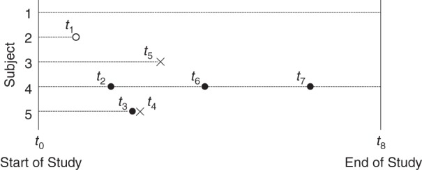
A visual representation of a hypothetical study that has a recurrent-event outcome. A dashed line represents the follow-up period of each individual. A solid circle represents the occurrence of the event of interest, an open circle represents censoring, and a cross represents the occurrence of the competing-risk event.

First, we calculate the overall KM survival probability (Table 1). Note that when the event of interest occurs, it does not change the number of individuals at risk for the next time interval, because these individuals are still at risk for another occurrence of the event of interest. Next, we calculate the mean cumulative count of events per person by time t_j on the basis of equation 3 (Table 2).

Table 1.

Calculation of Overall Survival Probability

Time Interval		No. at Risk, nj − 1	No. Censored, cj	No. of Events of Interest, ej	No. of Competing-Risk Events, rj	Survival Probability, 1 – rj/nj − 1	Overall Survival Probability, KM(tj)
Time 1	Time 2	5	1	0	0	1	1
Time 2	Time 3	4	0	1	0	1	1
Time 3	Time 4	4	0	1	0	1	1
Time 4	Time 5	4	0	0	1	3/4	3/4
Time 5	Time 6	3	0	0	1	2/3	1/2
Time 6	Time 7	2	0	1	0	1	1/2
Time 7	Time 8	2	0	1	0	1	1/2
Time 8		2	2	0	0	1	1/2

Abbreviation: KM, Kaplan-Meier.

Table 2.

Calculation of Mean Cumulative Count

Time Interval		No. at Risk, nj − 1	No. of Events of Interest, ej	Probability of Event, ej/nj − 1	Survival up to tj, KM(tj − 1)	Average No. of Events, KM(tj − 1) × (ej/nj − 1)	Mean Cumulative Count, MCC(tj)
Time 1	Time 2	5	0	0	1	0	0
Time 2	Time 3	4	1	1/4	1	1/4	1/4
Time 3	Time 4	4	1	1/4	1	1/4	1/2
Time 4	Time 5	4	0	0	1	0	1/2
Time 5	Time 6	3	0	0	3/4	0	1/2
Time 6	Time 7	2	1	1/2	1/2	1/4	3/4
Time 7	Time 8	2	1	1/2	1/2	1/4	1
Time 8		2	0	0	1/2	0	1

Abbreviation: KM, Kaplan-Meier.

From Table 2, we see that MCC(t₈) = 1.0, which means that, by time t₈, the mean cumulative count of events of interest per person is estimated to be 1.0. In other words, because we have 5 individuals initially at risk, if we have no censoring, we would expect to see the event of interest occurring 5 times during follow-up, regardless of whether it was the first occurrence or not. Because the event of interest was experienced a maximum of 3 times in this example, we need to calculate only CumI₁(t_j), CumI₂(t_j), and CumI₃(t_j), and we illustrate that CumI₁(t_j) + CumI₂(t_j) + CumI₃(t_j) is equivalent to MCC(t_j) (Table 3).

Table 3.

Equivalence of the Sum of CumIs and MCC

Time Interval		CumI1(tj)	CumI2(tj)	CumI3(tj)	CumI1(tj) + CumI2(tj) + CumI3(tj)	MCC(tj)
Time 1	Time 2	0	0	0	0	0
Time 2	Time 3	1/4	0	0	1/4	1/4
Time 3	Time 4	1/2	0	0	1/2	1/2
Time 4	Time 5	1/2	0	0	1/2	1/2
Time 5	Time 6	1/2	0	0	1/2	1/2
Time 6	Time 7	1/2	1/4	0	3/4	3/4
Time 7	Time 8	1/2	1/4	1/4	1	1
Time 8		1/2	1/4	1/4	1	1

Abbreviations: CumI, cumulative incidence; MCC, mean cumulative count.

AN EXAMPLE OF USE IN PRACTICE

Study population

To illustrate the use of MCC and contrast it with the use of CumI, we use the Childhood Cancer Survivor Study, a large cohort study designed to investigate the long-term effects of cancer and therapy among 5-year survivors of childhood cancer. The Childhood Cancer Survivor Study cohort consists of 5-year survivors of childhood cancer diagnosed before the age of 21 years between 1970 and 1986 in one of 26 collaborating pediatric oncology centers. A detailed description of the Childhood Cancer Survivor Study design has been published previously (4, 12). The Childhood Cancer Survivor Study was approved by institutional review boards at the 26 participating centers, and participants provided informed consent.

Childhood cancer survivors are at increased risk for developing subsequent neoplasms following childhood cancer, including subsequent malignant neoplasms, nonmalignant meningioma, and nonmelanoma skin cancers (3, 4). The occurrence of subsequent neoplasms affects cancer survivors' quality of life, increases health-care service needs, and is a central issue for aging survivors (3, 13). Radiation therapy (RT) has been consistently reported to increase the risk of subsequent neoplasms (3, 14, 15). The MCC methodology that we propose can be used to understand the total burden of subsequent neoplasms among childhood cancer survivors by RT exposure.

Statistical analysis

Specifically, we report MCC and CumI estimates of any type of subsequent neoplasm for a cohort of 12,588 survivors, starting from their entry into the Childhood Cancer Survivor Study cohort (5 years after the original childhood cancer diagnosis) and followed for a total of 244,889 person-years, with a median of 19.9 years of follow-up time (interquartile range, 16.1–24.6 years). We stratified survivors by whether they received RT treatment (RT group) or not (no RT group) in the 5-year period following the childhood cancer diagnosis prior to their entry into the Childhood Cancer Survivor Study cohort. Death from any cause was treated as a competing-risk event for occurrences of subsequent neoplasms, and survivors were censored at the date of last contact.

Among 8,469 survivors who received RT treatment, 1,229 experienced at least 1 subsequent neoplasm, and a total of 2,112 occurrences of subsequent neoplasms were reported after entry into the Childhood Cancer Survivor Study cohort between January 1975 and August 2009. Of the 1,229 survivors with subsequent neoplasms, 840 (68.3%) experienced only 1 subsequent neoplasm, and 389 (31.7%) experienced multiple subsequent neoplasms. Among 4,119 survivors who did not receive RT treatment during the same time period, a total of 221 occurrences of subsequent neoplasms were reported among 178 individuals, of whom 147 (82.6%) experienced only 1 subsequent neoplasm and 31 (17.4%) experienced multiple subsequent neoplasms.

Figure 2A shows the estimated MCC curves and 95% confidence intervals calculated by bootstrapping individual survivors using the bootstrap percentile method (16). The MCC analysis with all subsequent neoplasm occurrences reveals that, by 39 years after diagnosis, there would be an average of 0.56 subsequent neoplasms occurring per survivor (MCC = 0.56), or more easily interpreted as an average of 56.0 subsequent neoplasms occurring per 100 survivors in the RT group, compared with 16.1 subsequent neoplasms per 100 survivors in the no RT group (MCC = 0.16). In other words, we would expect to observe more than 1 subsequent neoplasm for every 2 survivors in the RT group compared with less than 1 subsequent neoplasm for every 6 survivors in the no RT group. This result suggests that, 39 years after diagnosis, the number of subsequent neoplasms experienced by survivors who received RT treatment is approximately 3.5 times higher compared with the number experienced by survivors who did not receive RT treatment. Figure 2B shows the estimated CumI curves and 95% confidence intervals that include only the first subsequent neoplasm occurrence for each survivor. It reveals that the probabilities of developing at least 1 subsequent neoplasm 39 years after diagnosis are 0.26 in the RT and 0.10 in the no RT groups. Translated to numbers of subjects with at least 1 subsequent neoplasm per 100 survivors, similar to the above interpretation of MCC, we expect 26 out of 100 survivors to have at least 1 subsequent neoplasm event among the RT-exposed group. Refer to the Discussion section for comments on this MCC curve.

Figure 2.

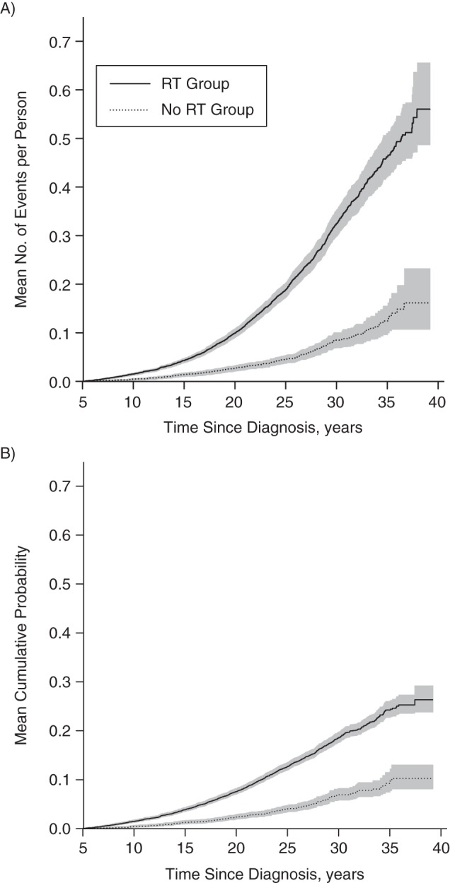
Estimated MCC curves and CumI curves based on data from the Childhood Cancer Survivor Study (26 pediatric oncology centers in the United States and Canada), 1975–2009. A) Mean cumulative count curves and 95% confidence intervals calculated by the bootstrap percentile method, stratified by whether received radiation treatment (RT group) or not (no RT group); B) cumulative incidence curves and 95% confidence intervals, stratified by RT group and no RT group. Gray shading represents 95% confidence intervals. CumI, cumulative incidence; MCC, mean cumulative count; RT, radiation therapy.

DISCUSSION

To capture the burden of recurrent events in a population occurring within a given time in the presence of competing risks, we discussed the use of MCC in this paper. Herein, we mathematically prove and empirically show the equivalence of the MCC and the sum of CumIs for the incremental number of events experienced within a population.

When analyzing data with recurrent events on the basis of the scientific questions of the study, one should first clearly establish whether the measure of primary interest is either 1) the percentage of people who experience the event of interest at least once or 2) a summary of the total number of events occurring within a population. For the former, CumI can be estimated; for the latter, the proposed MCC would be useful.

An important characteristic of the MCC, which is in contrast to the CumI, is that it is not a probability. The possible range of values for the MCC is not from 0 to 1 (this is the range of CumI that is a probability). Rather, it can be any positive number. This is because we are estimating the mean count of events per member of a certain population rather than the proportion of the population that develops the event of interest. Also, it is not interpretable without specification of the time period to which it applies. This is also true for CumI. Even when applied to the same population size, an average of 2 events per person can reflect a dramatically different burden of disease over a 50-year time period compared with a 1-year time period. From the illustrative example, we can see that a meaningful interpretation can be given as an average of 1 event per every X individuals initially at risk, or an average of Y events per 100 individuals initially at risk. For statistical inference with MCC, including the significance test and confidence intervals, we have easily applied the valid method of bootstrapping individuals (16). Ghosh and Lin (10) derived a 2-sample test.

Differences between MCC and CumI become larger as the repeated occurrence of events is more frequent. As shown in Figure 2 of the Childhood Cancer Survivor Study example, MCC in the no RT group led to a similar estimate as CumI, while they differed appreciably in the RT group. This reflects the more frequent repeated occurrences of subsequent neoplasms in the RT group relative to the no RT group, where few subjects had more than 1 subsequent neoplasm. In addition, the discrepancy between MCC and CumI becomes greater over time. Thus, the CumI analysis that incorporates only the first occurrence of subsequent neoplasms would underestimate the total burden of subsequent neoplasms more severely with longer follow-up time.

For quantifying the incidence of recurrent events, a traditional measure in epidemiology is a “rate” that is defined as the total number of events divided by the total person-time at risk for the event (2). The denominator takes into account the number of individuals in a cohort, as well as the length of time contributed by each individual. Rate reflects the fundamental force of all events of interest occurring in a population, and it can rise or fall with time. This is different from the MCC in this paper, as the denominator of MCC depends only on the number of individuals at risk. MCC reflects the average burden of the event of interest in a population, and it is a cumulative measure that cannot decrease with the length of the risk period. For regression analysis, different ways to extend Cox regression to recurrent-event settings have been proposed. For example, Wei et al. (17) proposed a marginal approach to multivariate failure time data with the use of a sandwich-type estimator of the variance-covariance matrix of regression coefficients. Application of this method to recurrent-event settings has been evaluated carefully with a conclusion that it is well justified (18). Refer also to the report by Therneau and Grambsch (19) for a summary of and comparison between different ways of extending Cox regression to recurrent-event settings, including the approach of Wei et al.

Note that MCC is a marginal measure (as opposed to a conditional measure) of disease burden, similar to CumI, and its interpretation is not conditional on survival free of competing-risk events (20). Also, MCC does not assume independence between the event of interest and the competing-risk events (9, 10). Thus, in our example from the Childhood Cancer Survivor Study, MCC is applicable to the situation where the event of interest (subsequent neoplasm) and the competing-risk event (death) are certainly correlated.

In real data analyses, censoring is common. While we assumed no censoring in providing the intuitive explanation of MCC as the sum of CumIs, it is pertinent to discuss what happens with censoring. Suppose there are 3 subjects who each develop 1 event of interest at times t₁, t₂, and t₃, respectively, with no censoring. The observed average number of events per subject by time t (>t₃) is 1.0, where the average goes up by one-third at t₁, t₂, and t₃. This is the estimate of MCC, and also that of CumI, at t. Now consider a different scenario where the subject who had an event at time t₁ was subsequently censored before time t₂. The estimate of MCC will go up by one-half, not one-third, at t₂ because the subject with an event at t₁ has been censored (i.e., assumed to have the same event processes as the other 2 who remained under study after the censoring time) and 1 event occurred in the 2 subjects under study at risk at t₂. Note that CumI does not change by censoring after an event occurrence. Thus, censoring increases the height of each jump of MCC estimates at subsequent event occurrences.

In some cases, the sum of CumIs rather than MCC estimates may be of interest. In fact, the MCC curve we presented in the Childhood Cancer Survivor Study above is the sum of CumIs. The sum of CumIs distinguishes the order of events within a person, while MCC considers all events to be exchangeable. Since a second cancer treatment may affect the risk of third and subsequent cancers, we felt that the sum of CumIs was more appropriate in the example. The sum of CumIs does, however, take censoring into account: It does so differently from MCC. Specifically, if a subject was censored after his/her pth event before the (p + 1)th event, this censoring will increase the height of the jumps of MCC estimates at every subsequent event occurrence by any subject, regardless of the number of events that individual had already experienced. For the sum of CumIs, however, this censoring will increase the jumps of CumI(p + 1), CumI(p + 2), CumI(p +3), …, but not those of CumIp, CumI(p − 1), CumI(p −2) at subsequent event occurrences. This also implies a precise condition where a censoring event does not make MCC and the sum of CumIs different: When a censoring event occurs after all subjects have experienced their pth event but before any subject experiences his/her (p + 1)th event for a natural number p, then this censoring will cause no difference between MCC and the sum of CumIs.

Finally, the MCC provides an additional approach for describing the occurrence of an outcome that can occur more than once during the period of observation. We do not propose that the MCC should replace other metrics such as the CumI, standardized incidence ratio, or absolute excess risk in describing the occurrence of an outcome. Rather, the MCC provides a new dimension, which reflects a total burden of the event of interest within a population. We provide a computation code of MCC with an illustrative example at https://ccss.stjude.org/resourcetools.

Note added in proof: After initial online publication of this article, we noted that a key assumption pertaining to the mathematical proof presented in the Appendix was missing. The proof showed that the sum of cumulative incidence and the mean cumulative count method were identical. We have now incorporated the assumption into the proof and have added an explanation to the text on how the 2 methods differ and on the use of each method when the assumption is not met.

APPENDIX

Proof of Equality in Equation 8

We assume that there are n₀ individuals initially at risk in the study. Each individual could experience 3 distinct kinds of events at time t_j during follow-up: 1) occurrence of the event of interest; 2) occurrence of a competing-risk event; and 3) censoring. However, we assume no censoring here.

The times at which any of the events occur can be ordered as t₁ ≤ t₂ ≤ … ≤ t_n.

Individuals could experience the event of interest (outcome 1 above) multiple times and remain in the study. However, they can experience outcome 2 or 3 only once. We further define the following:

• e_j: The number of events of interest at time t_j (first ever or recurrent);

• r_j: The number of individuals who experience a competing-risk event at time t_j; and

• n_j: The number of individuals who are at risk and under observation of the study beyond time t_j.

If we assume that an individual can experience at most m times of the recurrent event in the study, for the pth (p = 1, 2, …, m) occurrence of the event of interest:

• e_pj: The number of individuals who experience the pth event of interest at time t_j;

• r_pj: The number of individuals who experience a competing-risk event at time t_j (before experiencing p occurrences of the event of interest); and

• n_pj: The number of individuals who are under study beyond time t_j (i.e., have not experienced p occurrences of the event of interest or a competing-risk event).

For calculating CumI_p(t), we treat only the pth occurrence of the event as the event of interest. The population at risk for the pth occurrence of the event would consist of those individuals who have had the (p − 1)th occurrence of the event of interest, and after having the pth event, the individuals would leave the population at risk for the pth occurrence of the event.

Because there are n₀ individuals initially at risk, we have n_p0 = n₀. Note that e_j is the number of events of interest by time t_j, regardless of whether it was the first occurrence or not; therefore, we have $e_j={\sum }_{p=1}^m{e}_{pj}$.

Now, we want to mathematically prove that the MCC at time t is equivalent to the sum of CumI_p(t)s, such that

$$\text{MCC}(t)=\sum _{p=1}^m\text{Cum}{\text{I}}_p(t).$$

Here, CumI_p(t) represents the CumI for the pth (p = 1, 2, …, m) occurrence of the event of interest by time t.

On the basis of the formula for calculating MCC(t) and CumI(t), we have

$$\text{MCC}(t)=\{\begin{array}{cc}0& \text{if}s=0\\ \frac{e_1}{n_0}& \text{if}s=1,\\ \frac{e_1}{n_0}+\sum _{j=2}^s\frac{e_j}{n_{j-1}}\prod _{k=1}^{j-1}\left(1-\frac{r_k}{n_{k-1}}\right)& \text{if}s\ge 2\end{array}$$

and

$$\sum _{p=1}^m\text{Cum}{\text{I}}_p(t)=\{\begin{array}{cc}0& \text{if}s=0\\ \sum _{p=1}^m\frac{e_{p1}}{n_{p0}}=\frac{e_{11}}{n_{10}}& \text{if}s=1,\\ \sum _{p=1}^m\frac{e_{p1}}{n_{p0}}+\sum _{p=1}^m\sum _{j=2}^s\frac{e_{pj}}{n_{p(j-1)}}\prod _{k=1}^{j-1}\left(1-\frac{r_{pk}}{n_{p(k-1)}}\right)\prod _{k=1}^{j-1}\left(1-\frac{e_{pk}}{n_{p(k-1)}}\right)& \text{if}s\ge 2\end{array}$$

where s is the largest j such that t_j < t.

Mathematical induction is applied for the following proof.

Basis step: When s = 1, because e₁₁ = e₁ and n₁₀ = n₀, we have $\text{MCC}(t)={\sum }_{p=1}^m\text{Cum}{\text{I}}_p(t)$.

Inductive step: We assume that the equation holds for s = i, which means $\text{MCC}(t_i)={\sum }_{p=1}^m\text{Cum}{\text{I}}_p(t_i)$. For s = i + 1, we have

$$\text{MCC}(t_{i+1})=\text{MCC}(t_i)+\frac{e_{i+1}}{n_i}\prod _{k=1}^i\left(1-\frac{r_k}{n_{k-1}}\right)$$

$$\sum _{p=1}^m\text{CumI}(t_{i+1})=\sum _{p=1}^m\text{CumI}(t_i)+\sum _{p=1}^m\frac{e_{p(i+1)}}{n_{pi}}\prod _{k=1}^i\left(1-\frac{r_{pk}}{n_{p(k-1)}}\right)\prod _{k=1}^i\left(1-\frac{e_{pk}}{n_{p(k-1)}}\right).$$

By definition,

$$n_{pi}=n_i\times P(\text{being}\text{at}\text{risk}\text{fo}rp\text{th}\text{event}\text{at}t=i|\text{being}\text{at}\text{risk}\text{for}\text{an}\text{event}\text{at}t=i).$$

The above conditional probability can be calculated by

$$\frac{{\prod }_{k=1}^i(1-r_{pk}/n_{p(k-1)}){\prod }_{k=1}^i(1-e_{pk}/n_{p(k-1)})}{{\prod }_{k=1}^i(1-r_k/n_{k-1})}.$$

Because $e_{i+1}={\sum }_{p=1}^m{e}_{p(i+1)}$ and $\text{MCC}(t_i)={\sum }_{p=1}^m\text{Cum}{\text{I}}_p(t_i)$, we can show that $\text{MCC}(t_{i+1})={\sum }_{p=1}^m\text{Cum}{\text{I}}_p(t_{i+1})$.

In summary, we conclude that the MCC is equivalent to the sum of the CumIs for incremental numbers of events in the population.

REFERENCES

- 1.Gooley TA, Leisenring W, Crowley J, et al. Estimation of failure probabilities in the presence of competing risks: new representations of old estimators. Stat Med. 1999;186:695–706. [DOI] [PubMed] [Google Scholar]
- 2.Rothman KJ. Epidemiology: An Introduction. New York, NY: Oxford University Press; 2012. [Google Scholar]
- 3.Friedman DL, Whitton J, Leisenring W, et al. Subsequent neoplasms in 5-year survivors of childhood cancer: the Childhood Cancer Survivor Study. J Natl Cancer Inst. 2010;10214:1083–1095. [DOI] [PMC free article] [PubMed] [Google Scholar]
- 4.Robison LL, Mertens AC, Boice JD, et al. Study design and cohort characteristics of the Childhood Cancer Survivor Study: a multi-institutional collaborative project. Med Pediatr Oncol. 2002;384:229–239. [DOI] [PubMed] [Google Scholar]
- 5.Broderick J, Brott T, Kothari R, et al. The Greater Cincinnati/Northern Kentucky Stroke Study: preliminary first-ever and total incidence rates of stroke among blacks. Stroke. 1998;292:415–421. [DOI] [PubMed] [Google Scholar]
- 6.Cumming RG, Kelsey JL, Nevitt MC. Methodologic issues in the study of frequent and recurrent health problems. Falls in the elderly. Ann Epidemiol. 1990;11:49–56. [DOI] [PubMed] [Google Scholar]
- 7.Glynn RJ, Buring JE. Ways of measuring rates of recurrent events. BMJ. 1996;3127027:364–367. [DOI] [PMC free article] [PubMed] [Google Scholar]
- 8.Nelson WB. Recurrent Events Data Analysis for Product Repairs, Disease Recurrences, and Other Applications. Vol. 10 Schenectady, NY: Society for Industrial and Applied Mathematics; 2003. [Google Scholar]
- 9.Cook RJ, Lawless JF. Marginal analysis of recurrent events and a terminating event. Stat Med. 1997;168:911–924. [DOI] [PubMed] [Google Scholar]
- 10.Ghosh D, Lin DY. Nonparametric analysis of recurrent events and death. Biometrics. 2000;562:554–562. [DOI] [PubMed] [Google Scholar]
- 11.Greenland S, Rothman KJ. Basic concepts. In: Rothman KJ, Greenland S, Lash TL, eds. Modern Epidemiology. 3rd ed Philadelphia, PA: Lippincott Williams & Wilkins; 2008:32–50. [Google Scholar]
- 12.Robison LL, Armstrong GT, Boice JD, et al. The Childhood Cancer Survivor Study: a National Cancer Institute–supported resource for outcome and intervention research. J Clin Oncol. 2009;2714:2308–2318. [DOI] [PMC free article] [PubMed] [Google Scholar]
- 13.Armstrong GT, Liu W, Leisenring W, et al. Occurrence of multiple subsequent neoplasms in long-term survivors of childhood cancer: a report from the Childhood Cancer Survivor Study. J Clin Oncol. 2011;2922:3056–3064. [DOI] [PMC free article] [PubMed] [Google Scholar]
- 14.Meadows AT, Friedman DL, Neglia JP, et al. Second neoplasms in survivors of childhood cancer: findings from the Childhood Cancer Survivor Study cohort. J Clin Oncol. 2009;2714:2356–2362. [DOI] [PMC free article] [PubMed] [Google Scholar]
- 15.Sklar CA, Mertens AC, Mitby P, et al. Risk of disease recurrence and second neoplasms in survivors of childhood cancer treated with growth hormone: a report from the Childhood Cancer Survivor Study. J Clin Endocrinol Metab. 2002;877:3136–3141. [DOI] [PubMed] [Google Scholar]
- 16.Good PI. Estimating population parameters. In: Resampling Methods: A Practical Guide to Data Analysis. 3rd ed New York, NY: Springer-Verlag; 2006:5–28. [Google Scholar]
- 17.Wei LJ, Lin DY, Weissfeld L. Regression analysis of multivariate incomplete failure time data by modeling marginal distribution. J Am Stat Assoc. 1989;84408:1065–1073. [Google Scholar]
- 18.Metcalfe C, Thompson SG. Wei, Lin, and Weissfeld's marginal analysis of multivariate failure time data: Should it be applied to a recurrent events outcome? Stat Methods Med Res. 2007;162:103–122. [DOI] [PubMed] [Google Scholar]
- 19.Therneau TM, Grambsch PM. Modeling Survival Data: Extending the Cox Model. New York, NY: Springer; 2000. [Google Scholar]
- 20.Pepe MS, Mori M. Kaplan-Meier, marginal, or conditional probability curves in summarizing competing risks failure time data? Stat Med. 1993;128:737–751. [DOI] [PubMed] [Google Scholar]