Generalized linear model for partially ordered data

Abstract

Within the rich literature on generalized linear models, substantial efforts have been devoted to models for categorical responses that are either completely ordered or completely unordered. Few studies have focused on the analysis of partially ordered outcomes, which arise in practically every area of study, including medicine, the social sciences, and education. To fill this gap, we propose a new class of generalized linear models—the partitioned conditional model—that includes models for both ordinal and unordered categorical data as special cases. We discuss the specification of the partitioned conditional model and its estimation. We use an application of the method to a sample of the National Longitudinal Study of Youth to illustrate how the new method is able to extract from partially ordered data useful information about smoking youths that is not possible using traditional methods.

1. Introduction

Partially ordered sets (posets) are perhaps one of the most commonly encountered yet under-recognized and under-reported structures in the statistics literature. Few analytic tools have been made available for handling posets, and even when they have existed, they were built around a limited number of prototypical problems—for example, [1]. Indeed, the lack of appropriate statistical tools for posets may explain their relatively minor role in the literature. Historically, posets appeared as early as the classification of intelligence within Piagetian theory [2]. If binary variables Y₁, Y₂ respectively indicate whether or not each of the componential developmental intelligences—sensorimotor and conceptual—is above a specific threshold value, then general developmental intelligence contains the following poset categories: 11, 10, 01, 00, in which 10 and 01 cannot be strictly ordered. Another example is the classification of drinking behavior in studies of alcoholism: nondrinker, former drinker, current social drinker, and current heavy drinker. Sampson and Singh [3] described a poset in a psychiatric application: no anxiety, mild anxiety, anxiety with depression, and severe anxiety. The poset structure of all three examples can be represented by the Hasse diagram in Figure 1, in which the four categories are indicated respectively by nodes 0, 1, 2, and 3.

Figure 1.

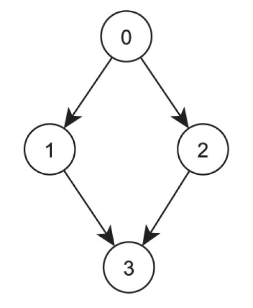
Four response categories form a poset structure.

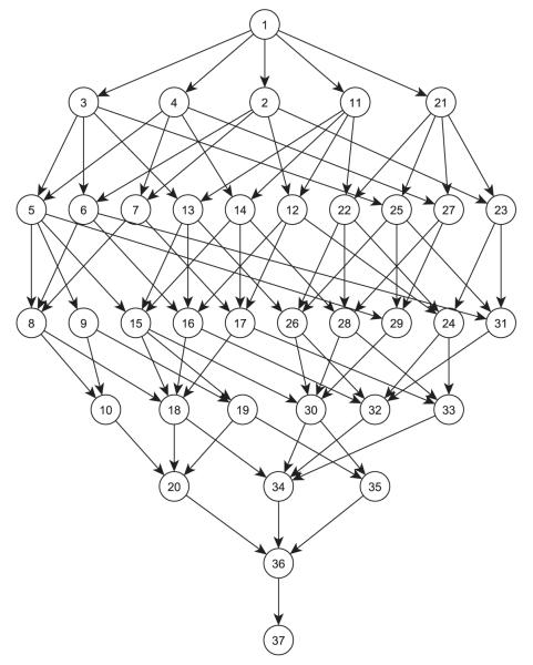
Posets could have far more complex structure than the four-category configuration shown in Figure 1. For example, in an application of posets to cognitive diagnosis, Tatsuoka [4] identified seven skills, coded A, B, … , G, necessary for a student to correctly compute subtraction of fractions in a mathematics test. Among the total 2⁷ = 128 states to master or not each one of the seven skills, 37 were identified from the test results data, and they are shown in Figure 2. Each node in the figure represents a state of mastery of a subset of the seven skills. State 1, for example, masters all seven skills; state 2 masters every skill except A; and state 5 masters every skill except E and C. The primary purpose of cognitive diagnosis is to classify each student into one of the 37 states so that remediation relating to specific deficit skills can be customized for each individual student.

Figure 2.

The Hasse diagram of a poset of 37 nodes, a replica of Figure 2 in [4].

1.1. Existing methods and their limitations

Because a poset arises naturally in response formats that contain multidimensional binary attributes, there is a substantial literature for treating a poset as multivariate binary data. Figure 3 shows the poset formed by the collection of three-dimensional binary responses. A common treatment of posets of this form is to create sum scores across the three binary responses so that a poset partitions itself into equivalent classes, each of which contains the nodes that have the same sum score—for example, [1]. Using this approach, the poset structure in Figure 3 is reduced to an ordinal response of four categories: 0,1,2,3. The ordinal data method can then be used to treat the sum score variable. An alternative approach, sometimes used in psychological testing, is to place constraints on posets. Using Figure 3 as an illustration, the Guttman scale [5] only considers the linearly ordered response patterns {000, 001, 011, 111}; the remaining patterns are considered either as not plausible or as simply a noisy version of the Guttman scale. An example of a Guttman scale is the scale for permissiveness of a state’s abortion regulation [6]. The scale contains questions about abortion under the following condition: a threat to the pregnant woman’s life, rape, or incest, a defective fetus or a risk to the woman’s physical health, a threat to the woman’s mental health, and free choice by the woman. Under the Guttman assumption, it is not possible for a respondent to endorse state regulation that allows abortion under a given criterion but to not endorse regulation that allows abortion under a higher level criterion.

Figure 3.

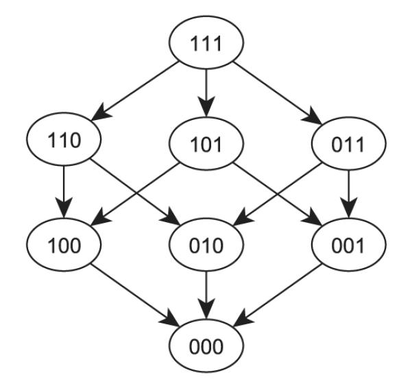
Eight response categories from a three-problem test.

Nonparametric statistical theories have also been developed to handle poset responses. Rosenbaum [7] studied properties of statistics such as rank sum of products for two-sample testing of poset data. Sampson and Singh [3] extended the rank-sum scoring method from ordinal data [8] to poset data. The authors also considered extreme-value statistics over all possible assignments of nondegenerate increasing scores for testing group differences. Except for very simple settings, both the sum score method and the Guttman scale approach have their own shortcomings. For example, it is unusual to find data that exhibit properties of the Guttman scale. For sum score, nuanced information contained in specific response patterns is lost through the summation process. Furthermore, there often exist posets that do not follow the multi-attribute response pattern. In Figure 2, these include state 6 master skills B, D, F, G, but not C and A, whereas skill E is undetermined. Using the sum score would put state 6 into the same score category as states that master four skills and do not master the remaining three skills (e.g., state 8). Both the sum score and the Guttman approach could not directly handle this kind of general posets.

Yet, another type of posets presents a challenge to the sum score and Guttman scale approaches— posets that contain disjoint substructures. An example of a disjoint poset in the literature is when a survey item contains not only ordinal categories (e.g., strongly agree to strongly disagree) but also a separate ‘Don’t know’ category. A sum score approach may have to adopt an ad hoc approach by either treating the response of ‘Don’t know’ as a missing value or collapsing it with one of the other response categories (e.g., neutral).

The approaches of [3] and [7] are rank-based methods and share many of the strengths and limitations of general nonparametric methods. The treatment of ties, for example, could be challenging. More importantly, both methods do not contain mechanisms of controlling for covariates. The methods also cannot directly handle poset responses with disjoint substructures. These limitations hinder their broader applications to clinical data.

In this paper, we propose a general class of partitioned conditional models (PCMs) for poset responses. The treatment of POS-PCM is rather general and includes generalized linear models (GLM) for nominal and ordinal responses as special cases. The extension of the GLM to posets significantly expands the power of GLM to include a rich class of responses that are common in neuorpsychological testing, clincial assessment, and other health surveys. The key idea of POS-PCM is to treat poset response as a new type of data, just like ordinal and categorical data types, and still be able to use well-developed models for the latter data types for statistical inference. Therefore, for a poset outcome such as that depicted in Figure 1, one can test the effectiveness of an intervention program for treating anxiety after controlling for baseline anxiety. In the following sections, we first describe some basic poset theory and then the development of POS-PCM through an example. We present a small simulation study that aims to validate the proposed estimation procedure and an application of POS-PCM to the National Longitudinal Study of Youth (NLSY).

2. Partially ordered set theory

A poset (P, ≤) is reflexive (a ≤ a), antisymmetric (if a ≤ b and b ≤ a, then a = b), and transitive (if a ≤ b and b ≤ c, then a ≤ c). When a ≤ b, we say that b dominates a. Two distinct elements, a and b in P, are comparable if a ≤ b or b ≤ a. Otherwise, they are incomparable. A poset with only a finite number of elements is called a finite poset. Henceforth, we only consider finite posets for their apparent connection with real applications.

An element a ∈ P is maximal (minimal) if there is no element b ∈ P such that a ≤ b (b ≤ a). In a finite poset, there is always at least one maximal element and one minimal element. The greatest lower bound (infimum) of a and b, if it exists, is denoted by a ∧ b and called their meet. Similarly, the supremum of a and b, if it exists, is their join, a ∨ b. A chain in a poset (P, ≤) is a totally ordered subset C of P, whereas an antichain is a set A of pairwise incomparable elements. A chain is a maximal chain if no other chain contains (covers) it. The Guttman scale mentioned in Figure 3 is a maximal chain. Similarly, we can define a maximal antichain. In Figure 3, the set {110, 101, 011} would be a maximal antichain. Figure 4(a) shows the poset structure of a four-category nominal response, where all four elements are incomparable, and hence the maximal chains are {0}, {1}, {2}, and {3}, and the maximal antichain is the entire set. Figure 4(b) shows a completely ordered four-category ordinal response, and hence the only maximal chain is C = {0, 1, 2, 3}, while there is no antichain.

Figure 4.

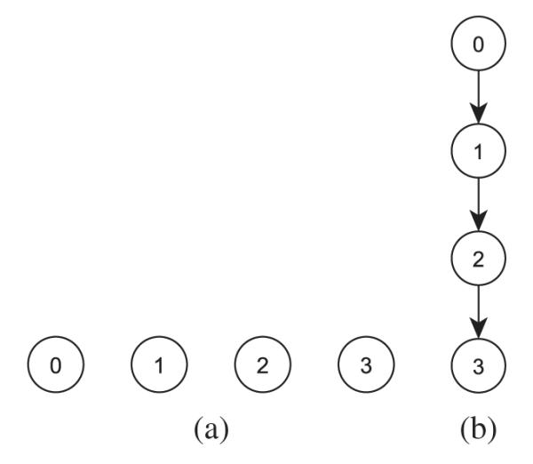
(a) Categorical responses from 0 to 3, (b) ordinal responses from 0 to 4.

A lattice is a poset in which any two elements have their meet and join. A finite lattice must have a unique maximal and a unique minimal [9]. Figures 1–3 are lattices that have a unique maximal on top and a unique minimal at the bottom. The height h(P) of a poset is the largest cardinality of a chain, and its width w(P) is the largest cardinality of an antichain. Thus, for a totally ordered finite set S, h(P) = ∣S∣ and w(P) = 1, whereas for an unordered set S, h(P) = 1 and w(P) = ∣S∣. In a finite poset, a chain C and an antichain A can have at most one element in common, and hence the least number of antichains to cover P is no less than h(P). The dual statement, Dilworth’s theorem [10], states that the cardinality of the largest antichain equals the least number of chains to cover P. Indeed, we can partition a poset P into antichains by recursively removing the set of maximal elements, which by definition is an antichain. Such a partitioning procedure, the specifics of which are to be described subsequently, is essential to the setting up of the POS-PCM.

To fix notation, define a weak order between subsets S₁ and S₂ in P if at least one element in S₂ is dominated by elements in S₁ and no element in S₂ dominates any element in S₁. We call it S₁ weakly dominates S₂. A set of subsets is called totally weakly ordered if pairwise subsets are weakly ordered. In Figure 3, the set of subsets {111}, {110, 101, 011}, {100, 010, 001}, and {000} is totally weakly ordered. Similarly, we define a strong order between S₁ and S₂ if every element in S₁ dominates all the elements in S₂, and we say that S₁ strongly dominates S₂. In Figure 3, the set of subsets {111}, {110, 011}, {010}, and {000} is totally strongly ordered. A set of subsets {A_i, i = 1, … , n} is called a partition of a poset P if ${\bigcup }_{i=1}^n{A}_i=P$ and $A_i\bigcap A_j=\varnothing$ for i ≠ j, and if a partition is at least totally weakly ordered, we call it an ordered partition.

To illustrate the aforementioned mathematical definitions, we use a real example of a poset represented in Figure 9(a), which we will discuss in detail in Section 4. The labeled categories concern smoker classification. Table I summarizes the illustration.

Figure 9.

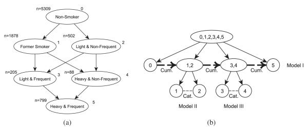
(a) A poset dominance structure for the National Longitudinal Study of Youth tobacco use variable. (b) The hierarchical model tree.

Table I.

Example (Figure 9(a)) for illustration of mathematical definitions.

Term	Example
Maximal element	Nonsmoker (0)
Minimal element	Heavy and frequent smoker (5)
Meet of (3) and (4)	Heavy and frequent smoker (5)
Join of (3) and (4)	Former smoker (1) and light and nonfrequent smoker (2)
Chain example	Nonsmoker (0) → former smoker (1) → light and frequent smoker (3)
Antichain example	{Former smoker (1), light and nonfrequent smoker(2)}
Maximal chain example	(0) → (1) → (3) → (5)
Maximal antichain example	{Former smoker (1), light and nonfrequent smoker(2)}
Height h(P)	4
Width w(P)	2
Weak dominance	{(1), (2)} Weakly dominates {(3), (4)}
Totally weakly ordered set	{{(0)}, {(1), (2)}, {(3), (4)}}
Strong dominance	{(1), (2)} Strongly dominates {(5)}
Partition of entire set	{{(0)}, {(1), (2)}, {(3), (4)}, {(5)}}

Proposition 1

(Ordered partition) A finite poset can always be partitioned into antichains that are totally weakly ordered.

Proof

Let A₁ be the set of maximal elements of P; by definition, it forms an antichain. By the definition of maximal, no element in P \ A₁ can dominate any element in A₁, and if P \ A₁ is nonempty, at least one element in P \ A₁ is dominated by elements in A₁, so we have P \ A₁ < A₁. The maximal elements A₂ of P \ A₁ are also weakly dominated by A₁. Recursively removing the set of maximal elements results in a set of {A_i} that is totally weakly ordered.

The set of {A_i} is an ordered partition. For example, in Figure 1, the three antichains A₁ = {0}, A₂ = {1, 2}, and A₃ = {3} form an ordered partition. In Figure 2, the partitions would be A₁ = {1},A₂ = {2, 3, 4, 11, 21}, … , A₈ = {37}. Apparently, these partitions are totally weakly ordered. It is worth pointing out here that the partitioning does not require any form of sum score and can generally be applied to all forms of finite posets.

By pointing out that (i) a finite poset can always be partitioned into antichains; (ii) the partitions are totally weakly ordered; and (iii) there exists a procedure for identifying the partitions through the iterative removal of the maximal element, Proposition 1 forms the basis for the construction of the formal PCM for POS. As we shall see, the PCM states that the poset is specified by a hierarchy of both nominal and ordinal models applied to the ordered partitioning antichains derived from Proposition 1—elements within individual antichains follow a nominal model, whereas ordered antichains follow an ordinal model.

2.1. Partitioned conditional models for posets

Instead of formally deriving the hierarchical ordinal and nominal models, it is easier to describe the modeling procedure using an example. Consider the poset in Figure 5, which contains three disjoint substructures, and further assume that a vector of covariates x is present. Operationalizing the PCM includes the following steps:

1. Partition the Hasse diagram into three disjoint networks : {0}, {1, .., 6}, and {7, 8}. Define π_ij = Pr(y_i = j∣x_i), for i = 1, … , N and j = 1, … , 8. Use one of the partitions, say {0}, as a reference category, specify the nominal model:

   $$\begin{array}{cc}\hfill \log \left(\frac{{\pi }_{i1}+{\pi }_{i2}+{\pi }_{i3}+{\pi }_{i4}+{\pi }_{i5}+{\pi }_{i6}}{{\pi }_{i0}}\right)& ={\beta }_0+x_i^{\prime }{\gamma }_0\hfill \\ \hfill \log \left(\frac{{\pi }_{i7}+{\pi }_{i8}}{{\pi }_{i0}}\right)& ={\beta }_1+x_i^{\prime }{\gamma }_1\hfill \end{array}$$ (1)
2. For the network {7, 8}, specify the conditional binary logit model:

   $$\log \left(\frac{{\pi }_{i7}}{{\pi }_{i8}}\right)={\beta }_2+x_i^{\prime }{\gamma }_2.$$ (2)
3. For the network {1, .., 6}, partition it into a set of totally weakly ordered antichains using Proposition 1: A₁ = {1, 2}, A₂ = {3, 4, 5}, and A₃ = {6}. Specify the following conditional proportional odds model:

   $$\begin{array}{cc}\hfill \log \left(\frac{{\pi }_{i1}+{\pi }_{i2}}{{\pi }_{i3}+{\pi }_{i4}+{\pi }_{i5}+{\pi }_{i6}}\right)& ={\beta }_3+x_i^{\prime }{\gamma }_3,\hfill \\ \hfill \log \left(\frac{{\pi }_{i1}+{\pi }_{i2}+{\pi }_{i3}+{\pi }_{i4}+{\pi }_{i5}}{{\pi }_{i6}}\right)& ={\beta }_4+x_i^{\prime }{\gamma }_3.\hfill \end{array}$$ (3)

   Note that the proportional odds model in Equation (3) can be easily generalized to any ordinal model.

4. Specify two conditional nominal models for each antichain derived from the partitioned subset {1, 2}:

   $$\log \left(\frac{{\pi }_{i1}}{{\pi }_{i2}}\right)={\beta }_5+x_i^{\prime }{\gamma }_4,$$ (4)
   and the subset {3, 4, 5}:

   $$\begin{array}{cc}\hfill \log \left(\frac{{\pi }_{i4}}{{\pi }_{i3}}\right)& ={\beta }_6+x_i^{\prime }{\gamma }_5,\hfill \\ \hfill \log \left(\frac{{\pi }_{i5}}{{\pi }_{i3}}\right)& ={\beta }_7+x_i^{\prime }{\gamma }_6.\hfill \end{array}$$ (5)

Figure 5.

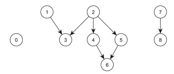
A poset dominance structure including three disjoint networks.

We graphically illustrate the procedure in Figure 6. In general, the procedure would be to first use Proposition 1 to partition a poset into a collection of totally weakly ordered antichains, which are modeled using an ordinal GLM. Within each antichain, the categories are then modeled using a nominal GLM. An appealing feature of the conditional approach is that the modeling process is consistent with a clinician’s mental model. For example, when faced with multiple (poset) categorization of a psychiatric disorder, a clinician would sort disorder categories approximately by their overall severity and subsequently compare different disorder categories that have more or less the same level of severity. The clinician might then want to examine the effects of various risk factors that drive general severity level and differentially affect the different disorder categories within the same of severity, perhaps using the most prevalent type as a reference category. Tutz [11] argued that for using conditional models for sequential reasoning, this kind of multiple stage, conditional thought process is well captured by the POS-PCM.

Figure 6.

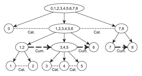
A hierarchical binary tree representation of the ordered partition process. The ‘Cat.’ and ‘Cum.’ labels are respectively used to indicate a categorical or cumulative model related to a split.

Two immediate questions concerning the POS-PCM modeling procedure need to be addressed: (i) how does one derive the individual category probability π_ij given the model parameters? and (ii) are the models within the POS-PCM identifiable?

To answer the first question, we again use the partition tree in Figure 6 as an illustrative example. We call the first node {0, 1, 2, 3, 4, 5, 6, 7, 8} the root node and each node within a branch a leaf. Let ${\mathcal{P}}_j$ denote a set of subsets of the original poset P that defines the path from the root to the leaf j in the partition tree and h(j) is the height of leaf j or equivalently the size of ${\mathcal{P}}_j$. For example, consider leaf 1. The path from the root to leaf 1 is

$${\mathcal{P}}_1=\left\{\right\{0,1,2,3,4,5,6,7,8\},\{1,2,3,4,5,6\},\{1,2\},\{1\left\}\right\}.$$

Thus, h(1) = 4. By tracing from the leaf 1 up to the root in the partition tree, the term π_i1 can be factorized as follows:

$${\pi }_{i1}=\frac{{\pi }_{i1}}{{\pi }_{i1}+{\pi }_{i2}}\frac{{\pi }_{i1}+{\pi }_{i2}}{{\pi }_{i1}+{\pi }_{i2}+{\pi }_{i3}+{\pi }_{i4}+{\pi }_{i5}+{\pi }_{i6}}\frac{{\pi }_{i1}+{\pi }_{i2}+{\pi }_{i3}+{\pi }_{i4}+{\pi }_{i5}+{\pi }_{i6}}{1},$$ (6)

where model (4) corresponds to the leftmost term, model (3) to the middle term, and model (1) to the rightmost term.

More generally, if we let ${\mathcal{P}}_{\mathit{jk}}$ denote the kth subset in ${\mathcal{P}}_j$, then ${\mathcal{P}}_{\mathit{jk}-1}$ is the parent set of ${\mathcal{P}}_{\mathit{jk}}$ and for all ${\mathcal{P}}_{j1}=P$. We further define ${\pi }_{{\mathcal{P}}_{\mathit{jk}}}={\sum }_{l\in {\mathcal{P}}_{\mathit{jk}}}{\pi }_{\mathit{il}}$ and write out the individual probabilities π_ij in a factored form:

$${\pi }_{\mathit{ij}}=\prod _{k=2}^{h\left(j\right)}\frac{{\pi }_{i{\mathcal{P}}_{\mathit{jk}}}}{{\pi }_{i{\mathcal{P}}_{\mathit{jk}-1}}},$$ (7)

where each factor on the right hand side (RHS) is a conditional probability:

$${\pi }_{i{\mathcal{P}}_{\mathit{jk}}}∕{\pi }_{i{\mathcal{P}}_{\mathit{jk}-1}}=\mathrm{Pr}(Y_i=j\in {\mathcal{P}}_{\mathit{jk}}\mid Y_i=j\in {\mathcal{P}}_{\mathit{jk}-1}).$$ (8)

For the second question concerning model identifiability, we have the following lemma.

Lemma 1

There are exactly K − 1 independent equations for a model with K response categories.

Proof

In the first ordered partition, we divide P into k + 1 antichains, which are modeled with a k-equation ordinal model. For elements within each antichain, we model them with a model having ∣A_i∣ equations. We know ${\sum }_{i=1}^k\mid A_i\mid =K-k-1$, and therefore there is a total of K − 1 independently specified equations.

The POS-PCM created from the partition-tree procedure is therefore identifiable.

3. Maximum likelihood estimation

McCullagh and Nelder [12] presented the loglikelihood for the POS-PCM:

$$l(y,\pi )=\sum _{i=1}^N\sum _{j=0}^{K-1}{y}_{\mathit{ij}}\log {\pi }_{\mathit{ij}},$$ (9)

where y_ij = 1 if y_i = j, and 0 otherwise, and y, π respectively represent the ensembles of y_ij and π_ij.

It can be shown that the loglikelihood can be decomposed into separate components such that each component can be maximized individually. Substituting π_ij in Equation (9) by the factored form in Equation (7), we have the following:

$$l(y,\pi )=\sum _{i=1}^N\sum _{j=0}^{K-1}{y}_{\mathit{ij}}\sum _{k=2}^{h\left(j\right)}\log \left(\frac{{\pi }_{i{\mathcal{P}}_{\mathit{jk}}}}{{\pi }_{i{\mathcal{P}}_{\mathit{jk}-1}}}\right).$$ (10)

Now, instead of using the ‘path’ index, reorganize the rightmost summation using the model index m = 1, … , K − 1:

$$l(y,\pi )=\sum _{i=1}^N\sum _{m=1}^{K-1}\sum _{j=0}^{K_m-1}{y}_{\mathit{imj}}\log {\widehat{\pi }}_{\mathit{imj}},$$ (11)

where ${\widehat{\pi }}_{\mathit{imj}}$ is the jth conditional probability specified in model m, y_imj = ∑_j∈Pmj y_ij, P_mj is the jth corresponding subset, and K_m is the number of categories in model m.

As an example, in Figure 6, the five models m = 1, … , 5, are respectively specified by Equations (1)–(5). Particularly, the conditional probabilities in model 3 are ${\widehat{\pi }}_{i31}=({\pi }_{i1}+{\pi }_{i2})∕{\sum }_{j=1}^6{\pi }_{\mathit{ij}},{\widehat{\pi }}_{i32}=({\pi }_{i3}+{\pi }_{i4}+{\pi }_{i5})∕{\sum }_{j=1}^6{\pi }_{\mathit{ij}}$, and ${\widehat{\pi }}_{i33}={\pi }_{i6}∕{\sum }_{j=1}^6{\pi }_{\mathit{ij}}$. The three corresponding subsets are P₃₁ = {1, 2}, P₃₂ = {3, 4, 5}, and P₃₃ = {6}.

From Equation (11), the summation contains K − 1 individual model loglikelihoods derived through the order partition procedure. If these models do not share common regression coefficients, then the maximum likelihood procedure separately maximizes each individual model loglikelihood of the form:

$$l_m(y,\pi )=\sum _{i=1}^N\sum _{j=0}^{K_m-1}{y}_{\mathit{imj}}\log {\widehat{\pi }}_{\mathit{imj}}.$$ (12)

Accordingly, existing software programs for estimation — nominal or cumulative logistic regression, respectively — can be directly applied to each individual model.

4. Data examples

4.1. Simulated data

We describe a small simulation experiment to demonstrate that the parameters of a POS-PCM can be accurately recovered using the estimation procedure.

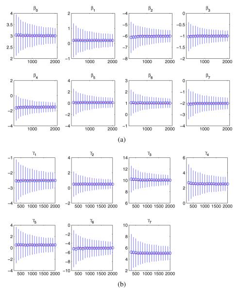
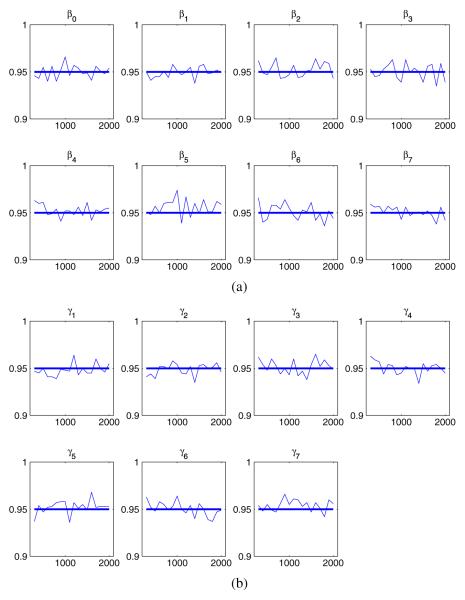
We generated a total of 1000 datasets, each of which had a sample size of n = 300, 400, 500, … , 2000, under the poset model represented by Figure 5. A single covariate x was randomly generated using a uniform distribution in [0, 1] and used across the simulated datasets. We used the MATLAB (The MathWorks Inc., Natick, MA, USA) function, ‘glmfit’, to fit binomial logit models in models (2) and (4), and the function, ‘mnrfit’, to fit multinomial ordinal and categorical models in models (1), (3)–(5). Figure 7 shows the comparisons of true βs and γs with the estimated means. Each vertical line indicates the 95%CI of an empirical mean estimate—that is, the range of ±1.96 times the empirical standard deviation, centered at the mean of the 1000 estimates. The estimated means (in circles) of the parameters are consistently close to the true values (as horizontal lines). The ranges, which approximately decrease as the square root of sample size, appear to indicate that the procedure is rather robust across the various models. Figure 8(a) and (b) shows the percentages of times when the true βs and γs are bracketed by the estimated 95%CI. The graphs show that the inference procedure produces a consistent type I error rate (0.05) across the parameters, suggesting that the confidence limits have correct coverage. All in all, the small simulation experiment demonstrates that parameters in POS-PCM can be accurately recovered when the model is correctly specified.

Figure 7.

(a) Plots of estimated means of βs in circles (true values in horizontal red lines), against sample size; (b) plots of estimated means of γs in circles (true values in horizontal red lines), against sample size.

Figure 8.

(a) Percentages of true β values covered by the estimated 95% confidence intervals; (b) percentages of true γ values covered by the estimated 95% confidence intervals. Horizontal axis indicates sample size.

4.2. National Longitudinal Study of Youth

We applied the POS-PCM to a data set that contains a sample of cohorts aged 12 to 16 years from the NLSY, a national survey of youths in the USA. We extracted three smoking-related variables: ever smoked (binary), the number of days smoked in the last 30 days, and the number of cigarettes smoked per day in the last 30 days. We used the variables to define a smoker classification variable that contains the following categories: nonsmoker, former smoker, light/nonfrequent smoker, light/frequent smoker, heavy/nonfrequent smoker, and heavy/frequent smoker. Figure 9(a) shows the poset lattice structure of the categories.

We identified the following variables as predictors in the POS-PCM: age, gender, race [13, 14], whether or not the child lives with both parents [15], mother’s support, mother’s permissiveness [16], whether or not the child is attending school [17], child’s attitude to discipline [18], and the number of smoking peers [14,19]. After removing subjects from the original sample of size 8984, with any missing data in either the outcome variables or the predictor variables, we obtained a subsample of size 8781 or 2% subjects with any missing data, and the top left corner of each node in Figure 9(a) shows the number of subjects in each category.

Following the order partitioning of Figure 9(b), we estimated the following three models:

• Model I. Proportional odds ordinal model for the four partitioned antichains—that is, nonsmokers coded as 0, former smokers and light/nonfrequent smokers together as 1, light/frequent smokers and heavy/nonfrequent smokers together as 2, and heavy/frequent smokers as 3.

• Model II. Nominal model for elements in the second antichain—that is, former smokers and light/nonfrequent smokers, with the latter as the reference category.

• Model III. Nominal model for elements in the third antichain—that is, heavy/nonfrequent smokers and light/frequent smokers, with the latter as the reference category.

Table II shows the estimated parameters and the associated standard errors.

Table II.

Estimated parameters from the National Longitudinal Study of Youth poset data set.

	Model I				Model II				Model III
	Estimate	SE	∣ t ∣	Pr > ∣t∣	Estimate	SE	∣ t ∣	Pr > ∣t∣	Estimate	SE	∣ t ∣	Pr > ∣t∣
Intercept 1	4.838	.305	15.858	< .001	.280	.690	.405	.685	−.279	1.876	.149	.882
Intercept 2	6.607	.309	21.384	< .001
Intercept 3	7.005	.310	22.604	< .001
Gender	.239	.045	5.261	< .001	.052	.103	.508	.612	.120	.272	.441	.659
Black versus White	.898	.058	15.498	< .001	−.190	.126	1.504	.133	.726	.373	1.946	.052
Hispanic versus White	.398	.058	6.806	< .001	−.257	.127	2.022	.043	.258	.350	.736	.462
Mixed versus White	−.098	.222	.439	.661	−.319	.484	.659	.510	N/A	N/A	N/A	N/A
Age	−.251	.018	13.959	< .001	.101	.040	2.514	.012	.874	1.074	.814	.416
Live with both parents	.163	.053	3.048	.002	−.010	.118	.087	.931	.276	.293	.940	.347
Nonsupportive mother	−.336	.043	7.878	< .001	−.100	.092	1.085	.278	.024	.247	.097	.923
Strict mother	.353	.040	8.741	< .001	.091	.091	1.003	.316	.414	.243	1.704	.088
Attend school	.569	.099	5.736	< .001	.053	.239	.220	.826	−.738	.662	1.114	.265
Negative attitude to discipline	−.316	.029	11.058	< .001	.024	.060	.405	.685	−.015	.167	.091	.928
Smoking peer	−.432	.020	21.896	< .001	−.175	.045	3.926	< .001	−.152	.125	1.216	.224

N/A is due to the absence of the mixed race among the subjects in model III.

SE, standard error; N/A, not applicable.

In the NLSY application, it is interesting to note that for model I, almost all of the predictors are significant. The finding is consistent with the literature for smoking. In the conditional model II, however, the only significant predictors are race (being Hispanic), age, and smoking peer. The last two variables both have negative impact on the odds ratio between former smoker and light and nonfrequent smoker, suggesting that having a smoking peer is a risk factor for a child to relapse into smoking if the child belongs to either one of the two smoking categories. These predictors are not significant any more under model III, which suggests that if a child is either a heavy/nonfrequent or a light/frequent smoker, none of the risk factors would lead to higher likelihood of being in one category or another. The result from analyzing the data using the POS-PCM can inform treatment and prevention strategies for children at various conditions and stages of smoking.

5. Discussion and conclusion

One limitation of the POS-PCM is that multiple poset structures could lead to the same models. Consider the example in Figure 9(a). If dominance links from ‘Former smoker’ to both ‘Light and frequent smoker’ and ‘Heavy and less frequent smoker’ were removed, the antichain would remain unaltered and so would the models.

The POS-PCM is perhaps most useful when the poset does not resemble a completely ordered or a completely segregated structure. Under such a situation, the POS-PCM could provide information about both the weakly ordered ‘between’ antichain effect and the unordered ‘within’ antichain effect. Using the smoking example, the first effect is useful for delineating general direction. For instance, a statistically significant coefficient for an intervention program would mean either significant improvement or deterioration in reducing smoking behavior. The second effect, on the other hand, can be used to examine differences in the influence of risk factors across outcome categories that are not necessarily ordered—for example, light and frequent versus heavy and nonfrequent smokers.

Like other conditional models, one should be careful about the interpretation of parameters of the POS-PCM. The parameter for a category within the nominal model only allows conditional interpretations—namely that the effect is conditional on the partition to which the category belongs. For example, in the NLSY example model II, a young person who has smoking peers is more likely to be a former smoker than a light/nonfrequent smoker given that the person belongs to either one of the two categories. Such ‘sequential’ interpretation might be appropriate in some but not in other situations [11].

It is worth pointing out here that the partial order structure of the outcome needs to be determined prior to applying POS-PCM to the data. As much as the ordering property of an ordinal outcome needs to be determined before applying an ordinal model—say the ordinal logistic regression—to the data, the POS-PCM approach does not select the poset structure. If response data do not have a predetermined structure, then it is still possible to select a structure using methods such as clustering. However, the topic will be beyond the scope of this paper.

In summary, we propose PCMs for partially ordered responses; this new class of models extends extant nominal and ordered categorical models and also inherits many of the properties of these existing models. The attractiveness of the proposed POS-PCM includes its flexibility and its leverage of the power of the GLM. This implies that methods developed for GLM, such as outlier detection, goodness of fit, and variable selection, can also be applied to the POS-PCM. The POS-PCM can also be brought to bear on rather complex poset structures that arise from a broad range of data. Although caution is required for the conditional interpretation of the regression coefficients, the POS-PCM can offer novel insight into poset response patterns when the models are properly interpreted.

References

- 1.Wilson M. The ordered partition model: an extension of the partial credit model. Applied Psychological Measurement. 1992;16(4):309. [Google Scholar]
- 2.Piaget J. The Psychology of Intelligence. Routledge and Kegan Paul; London: 1951. [Google Scholar]
- 3.Sampson AR, Singh H. Min and max scorings for two sample partially ordered categorical data. Journal of Statistical Planning and Inference. 2002;107(1–2):219–236. DOI: 10.1016/S0378-3758(02)00254-9. [Google Scholar]
- 4.Tatsuoka C. Data analytic methods for latent partially ordered classification models. Journal of the Royal Statistical Society Series C (Applied Statistics) 2002;51(3):337–350. DOI: 10.1111/1467-9876.00272. [Google Scholar]
- 5.Guttman LL. The basis for scalogram analysis. In: Maranell GM, editor. Scaling: A Sourcebook for Behavioral Scientists. Aldine Pub. Co.; Chicago: 1974. p. 142. [Google Scholar]
- 6.Mooney CZ, Lee M-H. Legislative morality in the American states: the case of pre-Roe abortion regulation reform. American Journal of Political Science. 1995;39(3):599–627. DOI: 10.2307/2111646. [Google Scholar]
- 7.Rosenbaum P. Some poset statistics. The Annals of Statistics. 1991;19(2):1091–1097. [Google Scholar]
- 8.Kimeldorf G, Sampson AR, Whitaker LR. Min and max scorings for two-sample ordinal data. Journal of the American Statistical Association. 1992;87(417):241–247. [Google Scholar]
- 9.Davey BA, Priestley HA. Cambridge mathematical textbooks. 2nd edn Cambridge University Press; 2002. Introduction to Lattices and Order. [Google Scholar]
- 10.Dilworth RP. A decomposition theorem for partially ordered sets. The Annals of Mathematics. 1950;51(1):161–166. [Google Scholar]
- 11.Tutz G. Sequential models in categorical regression. Computational Statistics & Data Analysis. 1991;11(3):275–295. DOI: 10.1016/0167-9473(91)90086-H. [Google Scholar]
- 12.McCullagh P, Nelder JA. Generalized Linear Models. 2nd edn Vol. 37 of Monographs on Statistics and Applied Probability. Chapman Hall; London: 1989. [Google Scholar]
- 13.Mermelstein R. Explanations of ethnic and gender differences in youth smoking: a multi-site, qualitative investigation. Nicotine and Tobacco Research. 1999;1:S91–S98. doi: 10.1080/14622299050011661. DOI: 10.1080/14622299050011661. [DOI] [PubMed] [Google Scholar]
- 14.Griesler PC, Kandel DB, Davies M. Ethnic differences in predictors of initiation and persistence of adolescent cigarette smoking in the National Longitudinal Survey of Youth. Nicotine and Tobacco Research. 2002;4(1):79–93. doi: 10.1080/14622200110103197. DOI: 10.1080/14622200110103197. [DOI] [PubMed] [Google Scholar]
- 15.Malik G. PhD Thesis. The Ohio State University; 2005. The role of parenting style in child substance use. [Google Scholar]
- 16.Newman IM, Ward JM. The influence of parental attitude and behavior on early adolescent cigarette smoking. Journal of School Health. 1989;59(4):150–152. doi: 10.1111/j.1746-1561.1989.tb04688.x. DOI: 10.1111/j.1746-1561.1989.tb04688.x. [DOI] [PubMed] [Google Scholar]
- 17.Gruber J, Zinman J. Youth smoking in the US: evidence and implications. National Bureau of Economic Research; 2000. p. 7780. (Working Paper Series). [Google Scholar]
- 18.Wang S-Q, Yu J-J, Zhu B-P, Liu M, He G-Q. Cigarette smoking and its risk factors among senior high school students in Beijing, China, 1988. Tobacco Control. 1994;3(2):107–114. [Google Scholar]
- 19.Powell LM, Tauras JA, Ross H. The importance of peer effects, cigarette prices and tobacco control policies for youth smoking behavior. Journal of Health Economics. 2005;24(5):950–968. doi: 10.1016/j.jhealeco.2005.02.002. DOI: 10.1016/j.jhealeco.2005.02.002. [DOI] [PubMed] [Google Scholar]