Abstract
Purpose
This work develops a compressive sensing approach for diffusion-weighted (DW) MRI.
Methods
A phase-constrained low-rank (PCLR) approach was developed using the image coherence across the DW directions for efficient compressive DW MRI, while accounting for drastic phase changes across the DW directions, possibly as a result of eddy current, and rigid and non-rigid motions. In PCLR, a low-resolution phase estimation was used for removing phase inconsistency between DW directions. In our implementation, GRAPPA was incorporated for better phase estimation while allowing higher undersampling factor. An efficient and easy-to-implement image reconstruction algorithm, consisting mainly of partial Fourier update and singular value decomposition, was developed for solving PCLR.
Results
The error measures based on diffusion-tensor-derived metrics and tractography indicated that PCLR, with its joint reconstruction of all DW images using the image coherence, outperformed the frame-independent reconstruction through zero-padding FFT. Furthermore, using GRAPPA for phase estimation, PCLR readily achieved a 4-fold undersampling.
Conclusion
The PCLR is developed and demonstrated for compressive DW MRI. A 4-fold reduction in k-space sampling could be readily achieved without substantial degradation of reconstructed images and diffusion tensor measures, making it possible to significantly reduce the data acquisition in DW MRI and/or improve spatial and angular resolutions.
Keywords: diffusion-weighted MRI, compressive sensing, low rank, phase correction, GRAPPA, diffusion tensor, tractography
Introduction
Diffusion-weighted (DW) MRI is a technique that allows the non-invasive mapping of the diffusion process of water molecules in biological tissues. This is achieved by applying a series of non-collinear diffusion-sensitive gradients to relate MRI signal attenuation to the water diffusion in the tissues of interest [1]. Because DW MRI can provide unique biologically and clinically relevant information in the living brain non-invasively, it has been widely applied in basic and clinical neuroscience for probing white matter integrity and connectivity of the brain [1-4]. One major obstacle of the technique, however, is the prolonged acquisition time. This is partially due to the fact that images need to be acquired with diffusion gradient applied in multiple directions to sufficiently sample the “diffusion space” in order to disentangle complex neuronal fiber crossings in the brain [5]. The scan time is even longer for several more sophisticated DW MRI techniques, including diffusion spectrum imaging (DSI) [6] and multi-shell Q-ball imaging [7], which require acquiring more than one shells of diffusion weighting. In addition, if high spatial resolution is desired, the segmented acquisition may be needed (i.e., covering the k-space in two or more segments), further increasing the data acquisition time. Thus, it is imperative to improve the DW MRI technique for reduced scan time and/or increased spatial and angular resolution without further time penalty.
Inspired by compressive sensing [8,9], compressive MRI with highly undersampled k-space has been actively pursued since 2006 [10]. Relevant to compressive DW MRI for reconstructing the DW images (x-q), the existing dynamic sparsity models for the spatiotemporal images (x-t) can be roughly classified into six categories. (1) The first dynamic sparsity model utilizes the 1D pixel-wise Fourier transform along the temporal dimension from the x-t space to the x-f space [11-13]. However, the temporal periodicity of x-t images, a key for the sparsity in the x-f domain, does not exist for DW images. (2) The second type uses the local sparsity up to certain transform, such as wavelet [10]. (3) The third is the adaptive local sparsity through dictionary learning [14]. (4) The fourth is the global sparsity via the low-rank model (LR) that involves singular value decomposition (SVD) of the x-t image along the temporal dimension [15,16]. (5) The fifth involves both the local sparsity and the global LR sparsity [17], which uses the supposition of both terms. (6) The last one is another use of both local and global sparsity, i.e., the rank-sparsity decomposition [18,19], where the image is modeled as two terms, assuming one term is globally sparse, e.g., the similar and stable background, and the other is locally sparse, e.g., the distinct and varying features. In the context of DW MRI, assuming no phase inconsistency between DW directions, we compared the above six models, and found that the LR model, a global sparsification of DW images via SVD, provides the best image reconstruction [20,21]. In addition, relative to the dictionary learning method for adaptive local sparsity, a prior-image constrained low-rank model was developed as an adaptive global sparsity method [22].
The sparsity model in DW MRI has been applied for image denoising [23,24], undersampling of DW directions [25-28], and undersampling of k-space [29-33]. With regard to undersampling of k-space, which is the focus of this work, various methods based on local and global sparsity have been developed, including local sparsity via total variation [29,30], tensor-model based image consistency [31], a mean-image based local sparsity, which is equivalent to a rank-one and sparsity decomposition [32], a PCA based global sparsity [32], and a group local sparsity, i.e., the L1 sum of L2 coefficients [33].
A major practical challenge for developing an efficient compressive DW MRI reconstruction method that uses the coherence between different diffusion directions is the drastic phase inconsistency between different DW directions as a result of eddy currents and the rigid and non-rigid motion. As a result, image coherence across the DW directions is destroyed, and all the above models are no longer valid, unless a phase correction is incorporated into the model. To the best of the knowledge, this phase problem has not been addressed for compressive DW MRI in the literature. This work describes the Phase-Constrained Low-Rank (PCLR) model that permits the use of coherence between different diffusion directions for compressive DW MRI.
Theory
The LR model takes advantage of image similarity, and thus is efficient for compressive 4D MRI [15-19]. Mathematically, LR is a convex minimization problem, in which the temporal similarity or coherence of the real part and the imaginary part of complex images can be enforced respectively through the nuclear norm, and the data fidelity term is linear with respect to the reconstruction variables, as the complex images are separated into the real and imaginary parts.
However, the existing LR is not applicable for compressive DW MRI. In DW MRI, there are drastic differences in the image phase between diffusion directions due to eddy currents and rigid and nonrigid body motion. As a result, the similarity of real or imaginary part no longer holds true, although the image magnitude is still coherent.
A plausible approach is to regularize the image magnitude while still reconstructing the real and imaginary part, in which the nuclear norm of the image magnitude acts similarly as the isotropic total variation. Unfortunately, from our experience, this approach is inadequate for image reconstruction, although the problem is still convex and linear.
Another logical direction is to reconstruct the magnitude and phase directly instead of the real and imaginary part, which may include the additional regularization of the phase, such as total variation. However, since the data fidelity is now non-linear in the magnitude and the phase, the problem becomes non-convex and the optimization is harder to solve. Again, our implementation on this has not been successful for satisfactory image reconstruction.
On the other hand, it is well known that the MR image phase can be approximated by a low-resolution phase with fairly good accuracy [34]. In the following, we will introduce the PCLR model, in which the low-resolution phase is used as a constraint in the nuclear norm regularization. That is the low-resolution phase is assumed to be a good approximation and utilized to compensate the drastic phase change, so that the complex DW images conjugated by the low-resolution phases regain the coherence in the DW gradient dimension. Please note that the low-resolution phase is not simply taken as the phase of the reconstructed images; rather it is used as a phase estimate and constraint to regain the DW similarity for better image reconstruction. In contrast, the final image phase was fixed to be a low-resolution one in [30]; in addition, the motivation of using the phase was to enable the model-based reconstruction, where the assumed diffusion tensor intensity model only applies to the amplitude.
K-space Sampling
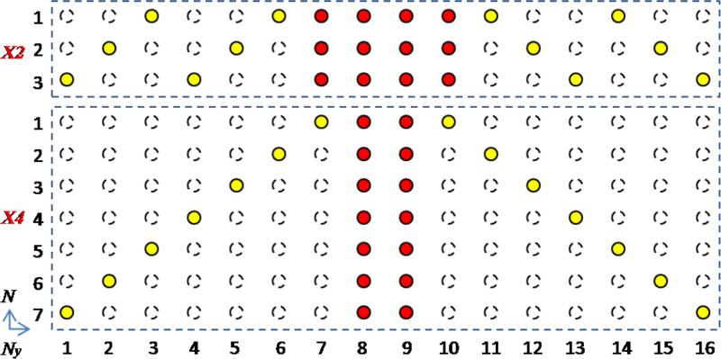
When using the LR method, it is desirable to have complementary k-space sampling with respect to the DW dimension, so that the common features across the DW dimension that may be missed otherwise due to undersampling can be recovered through LR. Meanwhile, the central k-space needs to be consistently sampled for PCLR, so that the low-resolution phase can be estimated as the phase constraint for PCLR.
The k-space sampling for PCLR is described in Fig. 1, and the modified version for PCLR that incorporates GRAPPA [35,36](GP-PCLR) is illustrated in Fig. 2. In both, the peripheral sampling is circulant with respect to the DW dimension, and is repeated every a few DW directions. Here the random sampling strategy is not used, since we find the circulant sampling strategy offers the comparable image quality, is more robust, and more straightforward for pulse sequence implementation.
FIG. 1.
K-space sampling for PCLR. For both 2-fold (X2) and 4-fold (X4) undersampling, the half of the data (red dots) is acquired at the central k-space, while the other half (yellow dots) is acquired at the peripheral k-space. The peripheral sampling is circulant with respect to the DW dimension, and is repeated every 3 or 7 DW directions for X2 and X4 respectively. The k-space with the central data (red dots) and zero-filling elsewhere is used to generate the low-resolution phase estimate. Then with PCLR, the image reconstruction utilizes all the data (red and yellow dots) to reconstruct the DW images.
FIG. 2.
K-space sampling for GP-PCLR. In this 4-fold (X4) undersampling example, the half of the data (red dots) is acquired at the central k-space, while the other half (yellow dots) is acquired at the peripheral k-space. Both the central and the peripheral sampling are circulant with respect to the DW dimension, and are repeated every 2 and 6 DW directions respectively. For reconstruction, GRAPPA is used to fill in the missing central data (blue dots), and the k-space with the central data (red and blue dots) and zero-filling elsewhere is used to generate the low-resolution phase estimate. Then with PCLR, the image reconstruction utilizes all the data (red, blue and yellow dots) to reconstruct the DW images.
To balance the low-frequency and high-frequency sampling, half of the data is acquired at the central k-space, while the other half is acquired at the peripheral k-space. For PCLR (Fig. 1), the central k-space is fully sampled, and the k-space with the central data and zero-filling elsewhere is used to generate the low-resolution phase estimate. Subsequently, with the phase-constrained image regularization, the image reconstruction utilizes all the acquired data to reconstruct the DW images. For GP-PCLR (Fig. 2), the central k-space is also circulantly undersampled with respect to the DW dimension. For image reconstruction, GRAPPA is used to fill in the missing central data; then the k-space with all the acquired and filled central data and zero-filling elsewhere is used to generate the low-resolution phase estimate. Then with the phase-constrained image regularization, the image reconstruction utilizes all the acquired and filled data to reconstruct the DW images.
PCLR Model
Let us start with some notations and definitions. X={xijkn, i≤Nx, j≤Ny , k≤Nz,m≤Nc,n≤N}, where Nc is the number of coils and N is the number of DW directions. Our data acquisition for DW MRI is independent with respect to different slices, i.e., Nz. To simplify the notation, let us consider the reconstruction of only one slice from one coil X={xijn, i≤Nx, j≤Ny, n≤N}, and then the other slices can be reconstructed in the same way. Here, although GRAPPA uses multiple-coil data for k-space interpolation, the reconstruction process after the k-space filling is still independent with respect to the coil. After coil-independent reconstruction, the images from all coils are combined through the simple sum-of-square formula [34].
Let Xn be an aligned column vector of each 2D DW image, and X be represented as a matrix, i.e., X=[X1··· Xn ··· XN]. The forward model is defined with the 2D Fourier transform matrix F and sampling matrix Sn, which is one for sampled k-space and zero for un-sampled k-space. We denote the forward model by AX=SFX=[S1FX1 ···SnFXn ··· SNFXN]. Let Y be the given data for the image reconstruction in the matrix format, i.e., Y=[Y1 ··· Yn ··· YN], where Yn is an aligned column vector of the nth 2D DW k-space, with the zero value at the un-sampled location. For GP-PCLR, the filled central k-space is also included in Y. On the other hand, let YC consists of the central k-space of Y and zero-filling elsewhere. Again the central part includes the filled data by GRAPPA for GP-PCLR.
A major challenge for developing an efficient LR method of compressive DW MRI is that the image phase changes drastically across the DW directions, which is a compound effect of eddy current and motion, and consequently similarity regularization of the real and imaginary part of the complex images cannot be justified in LR. This motivates the following PCLR model
| (1) |
where P is the low-resolution phase, which is computed from YC by P=F−1YC and then normalized by its magnitude, i.e., P=P/| P|. Here, ∥ ∥* is the nuclear norm for promoting the similarity in DW direction, which is defined as the sum of the singular values of the matrix; P*X is an element-wise multiplication rather than a matrix multiplication with * denoting the conjugate operation.
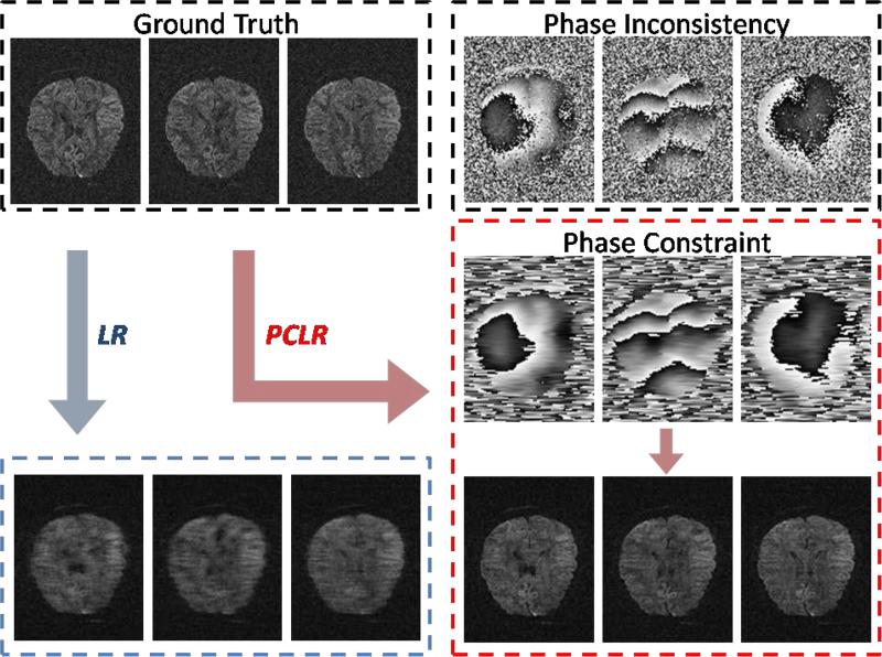
Here we consider an example to illustrate the importance of the phase constraint in Fig. 10, by comparing the reconstructed images between PCLR (with phase constraint) and LR (without phase constraint) using the 4-fold undersampling (Fig. 1). For LR, no phase information was used, i.e., P=I; for PCLR, the estimated phase using the acquired central k-space was utilized as the phase constraint P. Due to the phase inconsistency, LR failed to utilize the image similarity across the DW dimension. In contrast, through the phase constraint P to compensate the phase inconsistency, the image similarity across the DW dimension was recovered, and therefore the image quality was significantly improved by PCLR.
FIG. 10.
PCLR v.s. LR. The simulation data for image reconstruction are generated from the ground truth using 4-fold k-space undrsampling strategy (Fig. 1). In LR no phase information was used, while in PCLR the estimated phase using the acquired central k-space was utilized as the phase constraint. Due to the phase inconsistency, LR failed to utilize the image similarity across the DW dimension. In contrast, through the phase constraint to compensate the phase inconsistency, the image similarity across the DW dimension was recovered, and therefore the image quality was significantly improved by PCLR.
Solution Algorithm
In this section, we provide an efficient algorithm for solving PCLR (Eq. (1)), which mainly consists of partial Fourier update and singular value decomposition (SVD). The first trick is to reformulate the constrained problem Eq. (1) into the following unconstrained optimization with the Bregman update f
| (2) |
| (3) |
With the add-residual-back Bregman update of f via Eq. (3), the strategy of choosing a fixed regularization parameter λ is equivalent to the adaptive strategy of optimizing λ during iteration [37].
Secondly, Eq. (2) is split into a data fidelity minimization
| (4) |
and a nuclear norm minimization problem
| (5) |
The explicit solution to Eq. (5) is given by the singular value thresholding (SVT) formula [38], i.e.,
| (6) |
where the phase-conjugated image P*X is first decomposed with SVD, and the singular values are thresholded, i.e.,
| (7) |
Finally, Eq. (4) is reformulated as
| (8) |
And its explicit solution is given by
| (9) |
Eq. (9) is indeed a partial Fourier update [34], where the k-space data at the sampled location come from the acquired data Y, and the data at the un-sampled location come from the last iteration with the best data consistency.
To summarize, PCLR can be solved through the following simple single-loop solution algorithm
| (10) |
That is, PCLR (Eq. (1)) is solved iteratively with partial Fourier update, phase-constrained SVD, and add-residual-back Bregman update. The partial Fourier step provides the data fidelity, while the SVD step enforces the DW image similarity after the phase correction. Finally, the Bregman update is used to add the uncorrected residual back to be corrected, which is equivalent to optimize λ. Here it is apparent that the low-resolution phase P is used as the phase constraint rather than as the phase of reconstructed images. The algorithm Eq. (10) turns out to be a special case of the so-called Bregman operator splitting method [39] when applied to MRI, and therefore the convergence of the algorithm Eq. (10) is guaranteed. The equivalence proof is given in the Appendix.
In Eq. (10), the only parameter to be tuned is λ. However, the algorithm is robust with respect to λ, when the problem is properly scaled. That is the k-space data need to be scaled (i.e., multiplied by a constant) so that the maximum of the image magnitude is nearly one, which for example can be quickly determined through the inverse Fourier transform. Moreover, the algorithm is robust in λ, as long as λ is sufficiently large. The smaller the λ, the faster the convergence of the solution. Therefore, the solution algorithm Eq. (10) is nearly parameter-free, although an educated guess of λ will certainly accelerate the solution convergence with the reduced number of iterations. In this work λ is set to be one. On the other hand, the change of relative difference (i.e., ∥Xn+1-Xn∥) can be used as an efficient stopping criterion. That is, the iteration stops when the iterate difference no longer decreases significantly.
Methods
Data Acquisition
MRI was performed on a Siemens 3T Trio scanner (Siemens Medical System, Malvern, PA) with a twelve-channel phased-array coil. Foam cushions were used to minimize head motion. Diffusion MRI data were collected on a healthy male volunteer with a DW spin-echo EPI sequence. A dual spin-echo technique combined with bipolar gradients was used to minimize eddy-current effects [40]. The parameters used for diffusion data acquisition were as follows: DW gradients applied in 60 directions with a b value of 1,000 sec/mm2, repetition time/echo time of 10,800/114 msec, field of view of 256×256 mm2, matrix size of 128×128, resolution of 2×2×2 mm3, and 64 slices with no gap, covering the whole brain. Averages of two sets of DW images with phase-encoding directions of opposite polarity (left–right) were acquired to correct for susceptibility distortion [41]. The total diffusion MRI scan time was approximately 20 min.
Image Reconstruction
The acquired k-space was subsampled using the undersampling patterns in Figs. 1 and 2. For GP-PCLR, the GRAPPA algorithm was first applied to fill in the 4-fold undersampled central k-space: the non-acquired k-space values were estimated through a linear combination of nearby k-space values; the linear coefficients were found through a kernel fitting, with each kernel consisting of 4 neighboring blocks in the phase encoding direction and 7 nearest ones in the frequency encoding direction [36]; the b0 images were used as auto-calibration (ACS) lines to estimate the linear combination and the fitting was solved through the L2-regularizd least-squares. Subsequently, the k-space with the full central part and zero- filling elsewhere was used to generate the low-resolution phase estimate, and the k-space of all the sampled data (and the filled central part) was utilized in PCLR to reconstruct the DW images. The sumof-square formula [34] was used to combine the images from all coils to generate the magnitude images.
Image Analysis
Data preprocessing
The preprocessing of all DW MRI images retrospectively reconstructed by various methods was performed using Oxford Center for Functional Magnetic Resonance Imaging of the Brain's Software Library [42]. DW images were first corrected for eddy-current distortion. Susceptibility distortion was removed [41] using Matlab (Matlab7, Mathworks) codes incorporated in SPM5 [43]. This postprocessing technique for removing susceptibility-induced distortion takes advantage of the symmetric distortions in the two repetitions of diffusion MRI data with opposite phase encoding blips. The method generates images with a much higher geometric fidelity achievable using the conventional field map method [41,44]. Since (i) most diffusion imaging protocols need to acquire several repetitions for improved signal-to-noise ratio anyway and (ii) a relatively high angular resolution (60 diffusion directions) can be achieved with the current diffusion protocol incorporating the phase-reversal method, we incorporated this method in most diffusion MRI projects at our center.
Data analysis
Diffusion tensor and its derived metrics were calculated. We evaluated the performance of the zero-padding Fourier transform (FFT), PCLR and GP-PCLR under two k-space undersampling rates (50%, 25%), by comparing the root-mean-square-error (RMSE) of the reconstructed images, whole-brain fractional anisotropy (FA), mean diffusivity (MD), the principal diffusion direction (V1) and the diffusion tractography of the pyramidal tracts of the reconstructed data with those derived from images without undersampling. It should be noted that all analyses were conducted both before and after the merging of the two data sets with opposite phase encoding directions for susceptibility distortion correction. We reported only the results after the merging of the two data sets for susceptibility distortion correction because our tests showed almost identical trends in the data before the merging of the two repetitions, and the phase reversal method has become a standard post-processing technique for many diffusion MRI-related projects carried in our center.
We calculated the root-mean-squared-error (RMSE) of the whole brain, which is defined as:
| (11) |
where x and xi are the intensity of a voxel in the gold standard (full k-space sampling) and the corresponding reconstructed images. Low RMSE indicates more accurate reconstruction.
In our evaluations, we compared the fractional anisotropy (FA), mean diffusivity (MD) and the principal diffusion direction (V1) between the reconstructed images and the ground truth. We also traced the pyramidal tracts of the reconstructed data using FDT toolbox in FSL [42] and compared the results visually with the gold standard. It should be noted that the ball-and-stick partial volume model that enables the delineation of up to two crossing fibers, instead of the diffusion tensor model, was used in the tractography analyses [45]. A single seed voxel was placed in the middle of the corticospinal tract at the level of the pons and a waypoint mask at the posterior limb of internal capsule (PLIC) was drawn in each hemisphere to constrain the pyramidal tracts. Tracts traveling to the other side of the hemisphere were excluded in the final results. The resultant tracts were then normalized by the total number of the streamlines obtained in the results of the gold standard, and then thresholded at 5%. Maximal-intensity-projection (MIP) images of the normalized and thresholded results were then generated for qualitative comparisons.
Results
Raw diffusion images
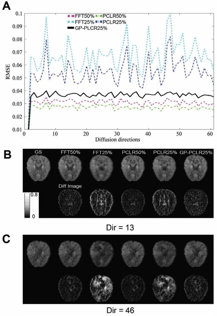
The RMSE across 60 diffusion directions are shown in Fig.3A, and the images at two representative directions (Dir=13, 46) are plotted in Fig.3B. Three major points can be made from the figure: (1) for 50% and 25% k-space undersampling rates, the PLCR method always outperforms the corresponding FFT method; (2) with the addition of GRAPPA, the GP-PCLR with a 25% undersampling rate significantly outperforms the PCLR and FFT methods at 25% undersampling rates without GRAPPA; (3) The performances of the PCLR and FFT vary significantly across diffusion directions when the sampled data in k-space is low (25%). For example, the RMSE in the diffusion direction 46 is almost twice as high as that in the diffusion direction 13, which could significantly affect diffusion-tensor-based metrics (see below).
FIG.3.
The root-mean-squared-error (RMSE) of the reconstructed raw diffusion and the difference images across diffusion directions. The RMSEs between the gold standard and the reconstructed diffusion raw images of the whole brain across DW gradients were calculated and plotted in (A). Different methods (FFT, PCLR, GP-PCLR) and sampling rates (50%, 25%) were compared. It can be seen that GP-PCLR 25% showed less RMSEs than the PCLR25% and FFT25%. The representative axial slices of the raw diffusion images (upper row) and the difference images (lower row) at two diffusion directions (Dir=13, 46) were also shown in Fig.B, C. Except that GP-PCLR generates low RMSEs, the performances of the method across the directions are more consistent across directions than the corresponding PCLR25% and FFT25%, which is critical for the accurate estimation of DTI-derived measures. The difference images were magnified four times for easy visualization.
DTI-derived metrics
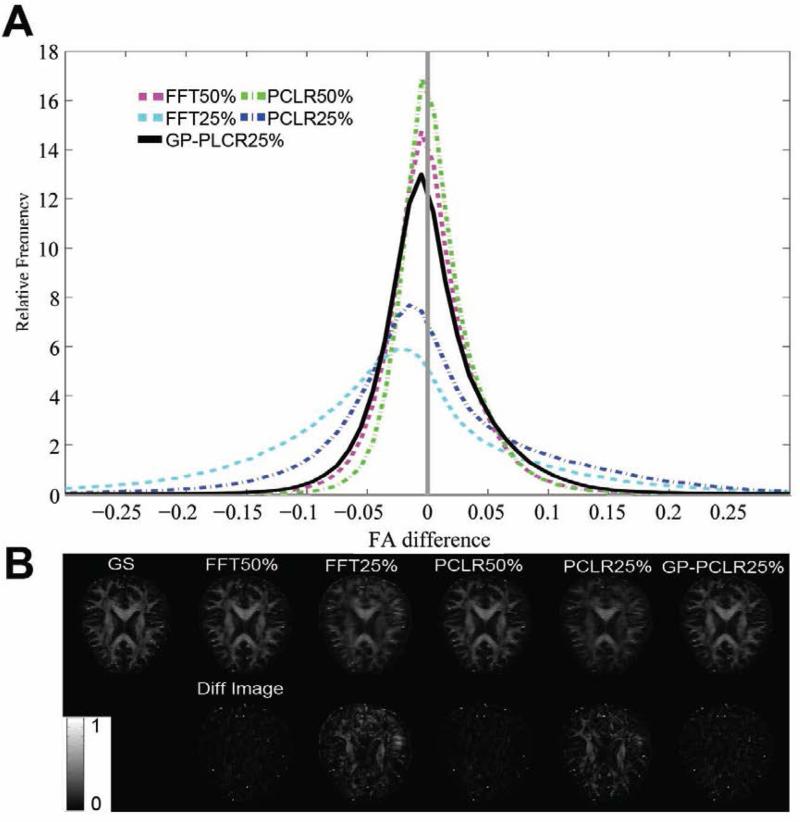
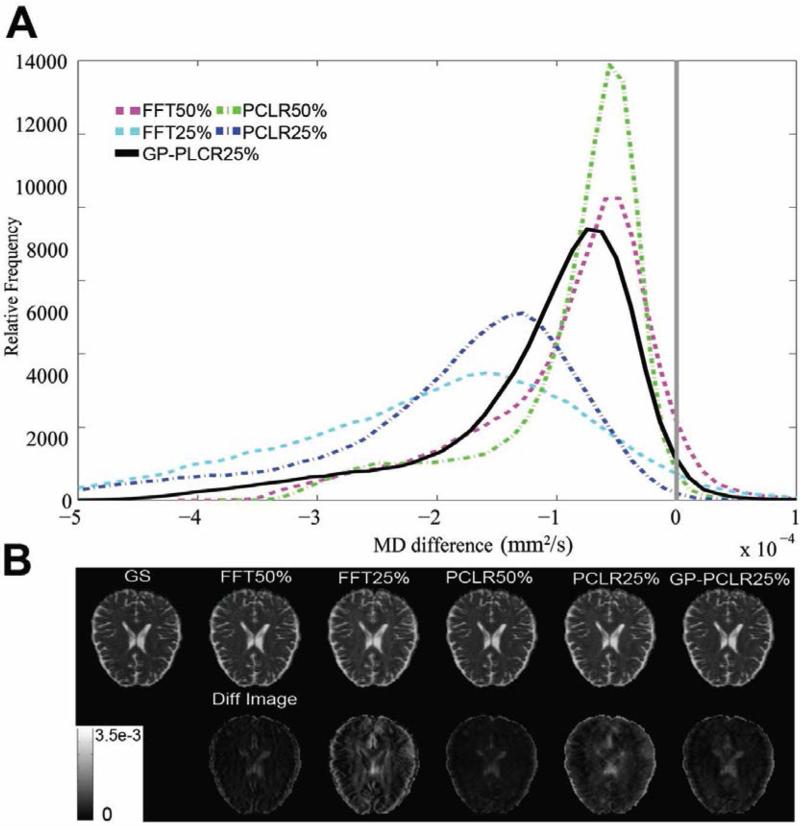
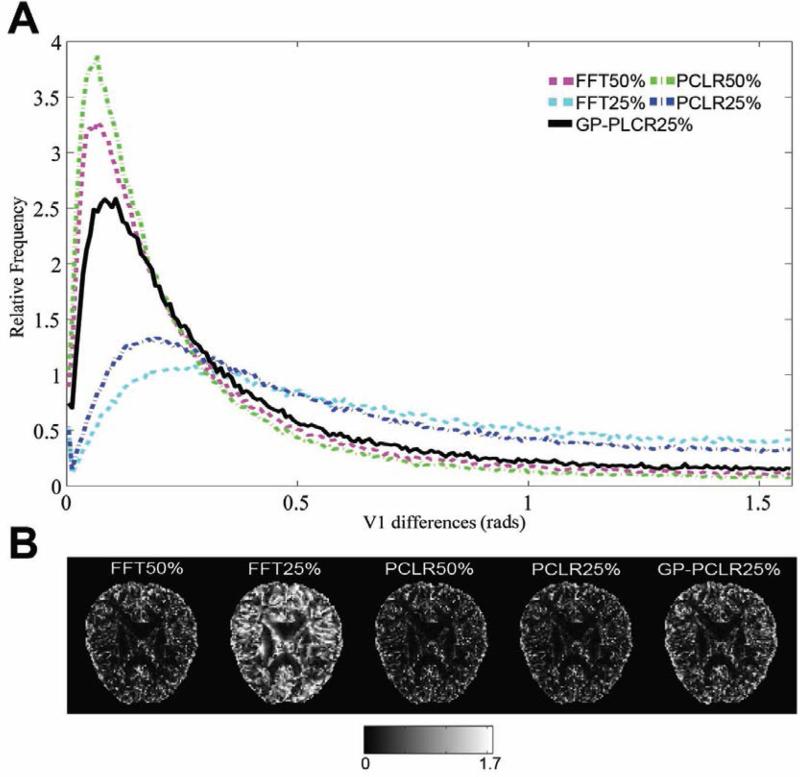
The histogram of the FA differences (gold standard – reconstructed images) of the whole brain, representative FA and difference images are shown in panels A and B of Fig.4. Consistent with the analyses based on the raw diffusion images, the PCLR method outperforms the corresponding FFT method at two undersampling rates (50%, 25%). The GP-PCLR with 25% achieved a performance similar as those by the PCLR and FFT method at 50% undersampling. It is interesting to see that for all compressive DW MR images, slightly more voxels in the brain have overestimated FA, which can be found to be mainly located at the gray matter of the brain (Fig.4B). The histogram of the MD differences (gold standard – reconstructed images) indicated that the majority of the voxels in the brain have overestimated MD, regardless of the method utilized (Fig.5). Similarly, GP-PCLR with a 25% undersampling performed better than PCLR and FFT at the same undersampling rate, and achieved a comparable performance to the PCLR and FFT methods at the 50% undersampling rate. We then compared the angular difference of the principal diffusion direction between the gold standard and the reconstructed images. It can be seen that for GP-PCLR method with 25% undersampling, the angular error is generally low in the deep white matter (~<6°) whereas in gray matter, it is much higher (~30°), which is consistent with the previous studies showing that diffusion tractography results are more reliable in deep white matter than in the gray matter of the brain [46] . The GP-PCLR with 25% undersampling rate consistently generated smaller angular error than those in the PCLR and FFT at 25% undersampling rate, as shown in Fig.6. Major contributions of the angular difference between the gold standard and the reconstructed images are in the gray matter areas, where isotropic diffusion is prominent (Fig. 6B).
FIG.4.
The FA differences between the reconstructed FA and the ground truth in the whole brain using different methods (FFT, PCLR, GP-PCLR) and undersampling rates (50%, 25%). Normalized histogram of FA differences across different methods and sampling rates are shown in (A). A narrow peak with a high relative frequency centered near zero indicates small differences between the ground truth and the reconstructed FA. PCLR25% and FFT25% tend to overestimate FA, whereas GP-PCLR25% showed close performance as that of FFT50%. The reconstructed FA maps (upper row) and the FA difference (lower row) in a representative slice are shown in (B). Compared to PCLR25% and FFT25%, GPPCLR25% showed less differences and the errors tend to be more homogenous across the brain than the former two methods. The FA differences were magnified twice for easy visualization. Note that FA is the ratio of anisotropic diffusion and therefore is unitless.
FIG.5.
The MD differences between the reconstructed images and the ground truth under various methods and undersampling rates. All reconstructed MD images tend to have overestimated MD in the most voxels in the brain. Compared to FFT25% and PCLR25%, GP-PCLR25% showed superior performance. The MD differences in a representative slice are shown in (B). The MD differences were magnified four for easy visualization.
FIG.6.
The angular differences of the principal diffusion direction (V1) in the diffusion tensor model between the reconstructed images and the ground truth under various methods and undersampling. A narrow peak with high relative frequency centered near zero indicates more accurate reconstruction. GPPCLR significantly outperformed the other two methods (PCLR and FFT) under the same sampling rate (25%) (A). A representative slice of the angular differences is shown in (B). Generally, the estimation of the V1 is more accurate in the white matter than in CSF and gray matter. The unit of B is in radians
Delineation of the pyramidal tracts using diffusion tractography
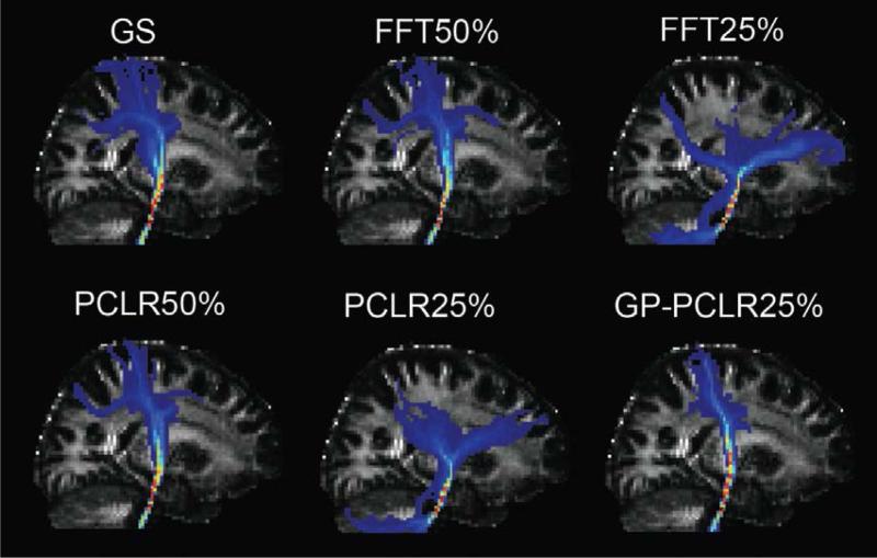
To further evaluate the impact of the reconstruction methods and undersampling rates on tractography analyses, we delineated the pyramidal tracts bilaterally using the data reconstructed by three methods (FFT, PCLR, GP-PCLR) and the two k-space undersampling rates (50%, 25%). From a seed voxel in the corticospinal tracts at the level of the pons, the pyramidal tracts pass through the superior cerebral peduncle dorsoventrally, the posterior limb of internal capsule and then project to both precentral and postcentral cortices (Fig. 7). When an undersampling rate of 50% was used, the pyramidal tracts could be faithfully tracked, regardless of the methods employed (FFT, PCLR). However, at the 25% of k-space sampling, we found that both FFT and PCLR methods were unable to reconstruct the pyramidal tracts accurately compared to the ground truth, with the major cortical connections diverted erroneously to the prefrontal cortex, instead of precentral and postcentral cortex (Fig.7). The GP-PCLR, on the other hand, is shown to be the only method that can reconstruct the main trajectory the tracts with such an undersampling rate (25%), although less connectivity to the postcentral gyrus was observed in the GPPCLR 25% reconstructed data.
Fig.7.
Comparisons of diffusion tractography on the pyramidal tracts using different reconstruction methods. A seed was placed in the corticospinal tracts at the level of pons. Then, waypoint masks at the posterior limb of the internal capsule were used to restrain the tracts. 10,000 streamline samples were sent from the seed voxel and the results were normalized using the total number of streamlines that were not rejected by the mid-sagittal exclusion mask in the ground truth. Then, the normalized tracts were thresholded at 0.5% and MIP images on the sagittal plane were plotted and compared. It can be seen that FFT 50% and PCLR50% generated most accurate results when compared to the ground truth. At the undersampling rate of 25%, GP-PCLR is the only method that enables a faithful reconstruction of the main course of the pyramidal tracts. In contrast, the tracts reconstructed by FFT25% and PCLR25% were significantly deviated from the original course, generating false connections to the prefrontal cortex and the cerebellum.
Discussions and Conclusions
In the present work, we developed and implemented a phase-constrained low-rank model for compressive reconstruction of DW MRI images. We systematically compared the performances of PCLR, GP-PCLR, and FFT at two undersampling rates (50%, 25%) based on a set of retrospectively undersampled diffusion data. Our results based on reconstructed images, DTI-derived metrics and tractography consistently demonstrated superior performances of PLCR compared to FFT.
Moreover, incorporation of GRAPPA with PCLR can further improve the performance of the PCLR, achieving a higher reduction of scan time and/or increased spatial and angular resolutions in DW MRI. It is possible that, instead of the explicit k-space filling and the explicit phase estimation using GRAPPA, an alternative strategy of incorporating the GRAPPA or SENSE as the multi-coil data or image consistency term into the reconstruction model [47] may be developed, which however may subject to the prior mentioned difficulty for solving magnitude-phase nonconvex optimization problem.
Our evaluations not only revealed the impact of the compressive sensing methodology on the resulting diffusion MRI-based measures, but also may help derive a “cutoff point” for the trade-off between the reconstruction accuracy and the k-space undersampling rates in evaluating compressive sensing methods. For example, while one may argue that the PCLR method with 25% k-space undersampling rate can produce diffusion MRI data with “decent” accuracy, our tractography analyses on the pyramidal tracts clearly demonstrated that the data based on such a method and undersampling rate would result in obvious false positive and negative connections that are against the classic neuroanatomical view of the pyramidal tracts, one of the most prominent projection fiber systems in the brain. Therefore, we can safely conclude that either the compressive sensing technique or the sampling rate needs to be modified for the technique to be useful. Indeed, with the incorporation of GRAPPA, GPPCLR with a 25% undersampling reconstructed the data that enable the tracking of the main pyramidal tracts accurately, suggesting its practical value in neuroscientific and clinical settings. On the other hand, with the reduced scanning time, the imaging artifacts due to motion could be also potentially reduced, which will be investigated in the future prospective studies using the proposed PCLR.
One major attraction of our proposed GP-PCLR method is the reduced scan time for either faster data acquisitions or increased spatial and angular resolutions in diffusion protocols. For example, assuming a similar diffusion protocol in the current study with the TR of 10800ms, b value of 1000, 64 slices, echo spacing of 1.16ms and a matrix size of 100×128, the GP-PCLR with 25% undersampling will take approximately 48% of the scan time required in the original diffusion protocol with full k-space sampling, This reduced scan time coupled with potentially minimized motion artifacts make the technique especially attractive in certain clinical settings such as pediatric and neonatal imaging. Phase inconsistencies due to eddy current and motion are common in a variety of MR imaging settings. The phase-constrained compressive reconstruction approach introduced here is generally applicable for compressive image reconstruction and complex image denoising when phase inconsistency poses a problem. For example, in cardiac imaging or fMRI, where cardiac or brain motion may induce phase variations between frames, the phase-constrained approach could be employed to further enhance the existing compressive sensing approaches.
Acknowledgments
This work is partially supported by NIH/NIBIB grant R21EB013387 and P50MH100029.
Appendix 1
Let us first consider the forward-backward operator splitting (FPOS) method [48] for solving
| (A1) |
That is, for any positive number δ, the FPOS method solves Eq. (A1), through decoupling Eq. (A1) into the following two iterative steps
| (A2) |
| (A3) |
Note that the algorithm is proven to converge when 0< δ<2/∥ATA∥ [48], which would be 0< δ<2 if A=F.
Let us consider the special case when δ=1. With A=SF, ST=S, STS=I, and FT=F−1, Eq. (A2) can be reformulated as
| (A4) |
On the other hand, with P*P=I, Eq. (A3) can be also reformulated as
| (A5) |
Next, after adding the add-residual-back Bregman update to Eq. (A4) and Eq. (A5), i.e., through the so-called Bregman operator splitting (BOS) method [39], we have
| (A6) |
which is the same as the solution algorithm Eq. (10). Therefore, the solution algorithm Eq. (10) is indeed equivalent to the BOS method.
Appendix 2
The phase-constrained model is generally applicable to the compressive sensing techniques. For example, for the local sparsity model with the wavelet transform W, the phase-constrained wavelet model, in analogy to Eq. (1), can be formulated as
| (A7) |
or
| (A8) |
For the sparsity transform satisfying WTW=I, the similar efficient algorithm to Eq. (10) can be derived, i.e.,
| (A9) |
In Eq. (A9), Tλ is the soft shrinkage formula, i.e., Tλ(x)=sgn(x)·max(|x-λ|,0) with the signum function sgn. Note that X is in the range of WT is assumed in order to derive the second step of Eq. (A9). The algorithm is again the same as the BOS method, with the derivation similar to Appendix 1.
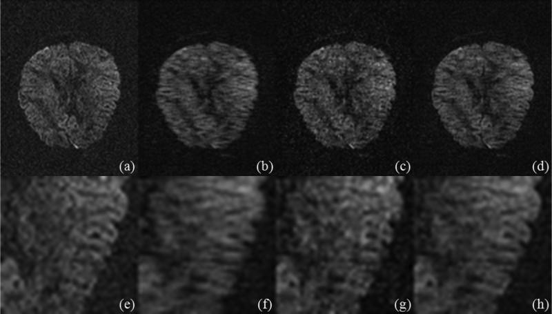
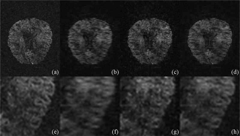
However, as suggested by our recent method comparisons [20,21], the LR model has a superior performance, which is also reflected through the qualitative comparison in Figs. 8 and 9 that correspond to the reconstructed images at 13th and 46th diffusion direction (Fig. 3) respectively from one repetition before the image postprocessing (e.g., the corrections of eddy-current and Susceptibility distortion) when using 25% data (Fig. 2). Here the three-level Haar wavelet transform is used in the phase-constrained wavelet model.
FIG.8.
The reconstructed images (without postprocessing) at the 13th diffusion direction with 25% data. (a) The ground truth; (b), (c), and (d) are from FFT, the phase-constrained wavelet model, and the PCLR respectively. (e-h) are their corresponding zoom-in details.
FIG.9.
The reconstructed images (without postprocessing) at the 46th diffusion direction with 25% data. (a) The ground truth; (b), (c), and (d) are from FFT, the phase-constrained wavelet model, and the PCLR respectively. (e-h) are their corresponding zoom-in details.
References
- 1.Basser PJ, Mattiello J, LeBihan D. Estimation of the effective self-diffusion tensor from the NMR spin echo. J Magn Reson. 1994;103:247–254. doi: 10.1006/jmrb.1994.1037. [DOI] [PubMed] [Google Scholar]
- 2.Mori S, Crain BJ, Chacko VP, Van Zijl P. Three-dimensional tracking of axonal projections in the brain by magnetic resonance imaging. Annals of Neurology. 1999;45:265–269. doi: 10.1002/1531-8249(199902)45:2<265::aid-ana21>3.0.co;2-3. [DOI] [PubMed] [Google Scholar]
- 3.Hagmann P, Cammoun L, Gigandet X, Meuli R, Honey CJ, Wedeen VJ, Sporns O. Mapping the structural core of human cerebral cortex. PLoS Biology. 2008;6:e159. doi: 10.1371/journal.pbio.0060159. [DOI] [PMC free article] [PubMed] [Google Scholar]
- 4.Kidwell CS, Alger JR, Di Salle F, Starkman S, Villablanca P, Bentson J, Saver JL. Diffusion MRI in patients with transient ischemic attacks. Stroke. 1999;30:1174–1180. doi: 10.1161/01.str.30.6.1174. [DOI] [PubMed] [Google Scholar]
- 5.Behrens TEJ, Berg HJ, Jbabdi S, Rushworth MFS, Woolrich MW. Probabilistic diffusion tractography with multiple fibre orientations: What can we gain? Neuroimage. 2007;34:144–155. doi: 10.1016/j.neuroimage.2006.09.018. [DOI] [PMC free article] [PubMed] [Google Scholar]
- 6.Wedeen VJ, Hagmann P, Tseng WYI, Reese TG, Weisskoff RM. Mapping complex tissue architecture with diffusion spectrum magnetic resonance imaging. Magn Reson Med. 2005;54:1377–1386. doi: 10.1002/mrm.20642. [DOI] [PubMed] [Google Scholar]
- 7.Jbabdi S, Sotiropoulos SN, Savio AM, Graña M, Behrens TE. Model-based analysis of multishell diffusion MR data for tractography: How to get over fitting problems. Magn Reson Med. 2012;68:1846–1855. doi: 10.1002/mrm.24204. [DOI] [PMC free article] [PubMed] [Google Scholar]
- 8.Candès EJ, Romberg J, Tao T. Robust uncertainty principles: Exact signal reconstruction from highly incomplete frequency information. IEEE Trans Inf Theory. 2006;52:489–509. [Google Scholar]
- 9.Donoho DL. Compressed sensing. IEEE Trans Inf Theory. 2006;52:1289–1306. [Google Scholar]
- 10.Lustig M, Donoho DL, Pauly JM. Sparse MRI: The application of compressed sensing for rapid MR imaging. Magn Reson Med. 2007;58:1182–1195. doi: 10.1002/mrm.21391. [DOI] [PubMed] [Google Scholar]
- 11.Lustig M, Santos JM, Donoho DL, Pauly JM. k-t SPARSE: high frame rate dynamic MRI exploiting spatio-temporal sparsity. Proc ISMRM. 2006:2420. [Google Scholar]
- 12.Gamper U, Boesiger P, Kozerke S. Compressed sensing in dynamic MRI,”. Magn Reson Med. 2008;59:365–373. doi: 10.1002/mrm.21477. [DOI] [PubMed] [Google Scholar]
- 13.Jung H, Sung K, Nayak KS, Kim EY, Ye JC. k-t FOCUSS: A general compressed sensing framework for high resolution dynamic MRI. Magn Reson Med. 2009;61:103–116. doi: 10.1002/mrm.21757. [DOI] [PubMed] [Google Scholar]
- 14.Ravishankar S, Bresler Y. MR image reconstruction from highly undersampled k-space data by dictionary learning. IEEE Trans Med Imaging. 2011;30:1028–1041. doi: 10.1109/TMI.2010.2090538. [DOI] [PubMed] [Google Scholar]
- 15.Liang ZP. Spatiotemporal imaging with partially separable functions. Proc ISBI. 2007:181–182. [Google Scholar]
- 16.Pedersen H, Kozerke S, Ringgaard S, Nehrke K, Kim WY. k-t PCA: Temporally constrained k-t BLAST reconstruction using principal component analysis. Magn Reson Med. 2009;62:706–716. doi: 10.1002/mrm.22052. [DOI] [PubMed] [Google Scholar]
- 17.Goud S, Hu Y, Jacob M. Real-time cardiac MRI using low-rank and sparsity penalties. Proc ISBI. 2010:988–991. [Google Scholar]
- 18.Gao H, Lin H, Ahn CB, Nalcioglu O. PRISM: A divide-and-conquer low-rank and sparse decomposition model for dynamic MRI. UCLA CAM Report. 2011:11–26. [Google Scholar]
- 19.Gao H, Rapacchi S, Wang D, Moriaty J, Meehan C, Sayre J, Laub G, Finn JP, Hu P. Compressed sensing using Prior Rank, Intensity and Sparsity Model (PRISM): applications in cardiac cine MRI. Proc ISMRM. 2012:2242. [Google Scholar]
- 20.Gao H, Li L, Hu X. Compressive diffusion MRI – part 1: why low-rank? Proc ISMRM. 2013:610. [Google Scholar]
- 21.Gao H, Li L, Hu X. Compressive diffusion MRI – part 2: performance evaluation via low-rank model. Proc ISMRM. 2013:2046. [Google Scholar]
- 22.Gao H, Li L, Hu X. Compressive diffusion MRI – part 3: prior-image constrained low-rank model (PCLR). Proc ISMRM. 2013:2605. [Google Scholar]
- 23.Haldar JP, Wedeen VJ, Nezamzadeh M, Dai G, Weiner MW, Schuff N, Liang ZP. Improved diffusion imaging through SNR-enhancing joint reconstruction. Magn Reson Med. 2012;69:277–289. doi: 10.1002/mrm.24229. [DOI] [PMC free article] [PubMed] [Google Scholar]
- 24.Lam F, Babacan SD, Haldar JP, Weiner MW, Schuff N, Liang ZP. Denoising diffusion-weighted magnitude MR images using rank and edge constraints. Magn Reson Med. 2013 doi: 10.1002/mrm.24728. doi: 10.1002/mrm.24728. [DOI] [PMC free article] [PubMed] [Google Scholar]
- 25.Saint-Amant E, Descoteaux M. Sparsity characterization of the diffusion propagator. Proc ISMRM. 2011:1915. [Google Scholar]
- 26.Landman BA, Bogovic JA, Wan H, ElShahaby FEZ, Bazin PL, Prince JL. Resolution of crossing fibers with constrained compressed sensing using diffusion tensor MRI. NeuroImage. 2012;59:2175–2186. doi: 10.1016/j.neuroimage.2011.10.011. [DOI] [PMC free article] [PubMed] [Google Scholar]
- 27.Menzel MI, Tan ET, Kedar K, Sperl JI, King KF, Tao X, Hardy CJ, Marinelli L. Accelerated diffusion spectrum imaging in the human brain using compressed sensing. Magn Reson Med. 2011;66:1226–1233. doi: 10.1002/mrm.23064. [DOI] [PubMed] [Google Scholar]
- 28.Michailovich O, Rathi Y, Dolui S. Spatially regularized compressed sensing for high angular resolution diffusion imaging. IEEE Trans Med Imaging. 2011;30:1100–1115. doi: 10.1109/TMI.2011.2142189. [DOI] [PMC free article] [PubMed] [Google Scholar]
- 29.Adluru G, Hsu E, DiBella EVR. Constrained reconstruction of sparse cardiac MR DTI data. Functional Imaging and Modeling of the Heart, Proceedings. 2007;4466:91–99. [Google Scholar]
- 30.Welsh CL, DiBella EVR, Adluru G, Hsu EW. Model-based reconstruction of undersampled diffusion tensor k-space data. Magn Reson Med. 2012 doi: 10.1002/mrm.24486. doi: 10.1002/mrm.24486. [DOI] [PMC free article] [PubMed] [Google Scholar]
- 31.Li Y, Aggarwal M, Mori S. Compressed sensing diffusion tensor imaging with tensor and phase constrains. Proc ISMRM. 2011:2840. [Google Scholar]
- 32.Pu L, Trouard TP, Ryan L, Bilgin A, Huang C, Altbach MI. Model-based compressive diffusion tensor imaging.. Proc of 8th International Symposium on Biomedical Imaging; Chicago, Illinois, USA. 2011.pp. 254–257. [Google Scholar]
- 33.Wu Y, Zhu YJ, Tang QY, Zou C, Liu W, Dai RB, Liu X, Wu EX, Ying L, Liang D. Accelerated MR diffusion tensor imaging using distributed compressed sensing. Magn Reson Med. 2013 doi: 10.1002/mrm.24721.. doi: 10.1002/mrm.24721. [DOI] [PubMed] [Google Scholar]
- 34.Bernstein MA, King KF, Zhou XJ. Handbook of MRI pulse sequences. Academic Press; 2004. [Google Scholar]
- 35.Griswold MA, Jakob PM, Heidemann RM, Nittka M, Jellus V, Wang J, Kiefer B, Haase A. Generalized autocalibrating partially parallel acquisitions (GRAPPA). Magn Reson Med 2002. 47:1202–1210. doi: 10.1002/mrm.10171. [DOI] [PubMed] [Google Scholar]
- 36.Nana R, Zhao T, Heberlein K, LaConte SM, Hu X. Cross-validation-based kernel support selection for improved GRAPPA reconstruction. Magn Reson Med. 2008;59:819–825. doi: 10.1002/mrm.21535. [DOI] [PubMed] [Google Scholar]
- 37.Osher S, Burger M, Goldfarb D, Xu J, Yin W. An iterative regularization method for total variation-based image restoration. Multiscale Modeling & Simulation. 2005;4:460–489. [Google Scholar]
- 38.Cai J-F, Candès EJ, Shen Z. A singular value thresholding algorithm for matrix completion. SIAM J Optimization. 2010;20:1956–1982. [Google Scholar]
- 39.Zhang X, Burger M, Bresson X, Osher S. Bregmanized nonlocal regularization for deconvolution and sparse reconstruction. SIAM Journal on Imaging Sciences. 2010;3:253–276. [Google Scholar]
- 40.Alexander AL, Tsuruda JS, Parker DL. Elimination of eddy current artifacts in diffusion-weighted echo-planar images: the use of bipolar gradients. Magn Reson Med. 1997;38:1016–1021. doi: 10.1002/mrm.1910380623. [DOI] [PubMed] [Google Scholar]
- 41.Andersson JLR, Skare S, Ashburner J. How to correct susceptibility distortions in spin-echo echo-planar images: application to diffusion tensor imaging. Neuroimage. 2003;20:870–888. doi: 10.1016/S1053-8119(03)00336-7. [DOI] [PubMed] [Google Scholar]
- 42. http://www.fmrib.ox.ac.uk/fsl/
- 43. http://www.fil.ion.ucl.ac.uk/spm/
- 44.Jezzard P, Balaban RS. Correction for geometric distortion in echo planar images from B0 field variations. Magn Reson Med. 1995;34:65–73. doi: 10.1002/mrm.1910340111. [DOI] [PubMed] [Google Scholar]
- 45.Behrens TEJ, Berg HJ, Jbabdi S, Rushworth MF, Woolrich MW. Probabilistic diffusion tractography with multiple fibre orientations: what can we gain? Neuroimage. 2007;34:144–155. doi: 10.1016/j.neuroimage.2006.09.018. [DOI] [PMC free article] [PubMed] [Google Scholar]
- 46.Behrens TEJ, Woolrich MW, Jenkinson M, Johansen-Berg H, Nunes RG, Clare S, Matthews PM, Brady JM, Smith SM. Characterization and propagation of uncertainty in diffusion-weighted MR imaging. Magn Reson Med. 2003;50:1077–1088. doi: 10.1002/mrm.10609. [DOI] [PubMed] [Google Scholar]
- 47.Lustig M, Pauly JM. SPIRiT: Iterative self-consistent parallel imaging reconstruction from arbitrary k-space. Magn Reson Med. 2010;64:457–471. doi: 10.1002/mrm.22428. [DOI] [PMC free article] [PubMed] [Google Scholar]
- 48.Combettes PL, Wajs VR. Signal recovery by proximal forward-backward splitting. Multiscale Modeling & Simulation. 2005;4:1168–1200. [Google Scholar]


