Investigating machine learning techniques for MRI-based classification of brain neoplasms

Abstract

Purpose

Diagnosis and characterization of brain neoplasms appears of utmost importance for therapeutic management. The emerging of imaging techniques, such as Magnetic Resonance (MR) imaging, gives insight into pathology, while the combination of several sequences from conventional and advanced protocols (such as perfusion imaging) increases the diagnostic information. To optimally combine the multiple sources and summarize the information into a distinctive set of variables however remains difficult. The purpose of this study is to investigate machine learning algorithms that automatically identify the relevant attributes and are optimal for brain tumor differentiation.

Methods

Different machine learning techniques are studied for brain tumor classification based on attributes extracted from conventional and perfusion MRI. The attributes, calculated from neoplastic, necrotic, and edematous regions of interest, include shape and intensity characteristics. Attributes subset selection is performed aiming to remove redundant attributes using two filtering methods and a wrapper approach, in combination with three different search algorithms (Best First, Greedy Stepwise and Scatter). The classification frameworks are implemented using the WEKA software.

Results

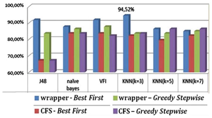
The highest average classification accuracy assessed by leave-one-out (LOO) cross-validation on 101 brain neoplasms was achieved using the wrapper evaluator in combination with the Best First search algorithm and the KNN classifier and reached 96.9% when discriminating metastases from gliomas and 94.5% when discriminating high-grade from low-grade neoplasms.

Conclusions

A computer-assisted classification framework is developed and used for differential diagnosis of brain neoplasms based on MRI. The framework can achieve higher accuracy than most reported studies using MRI.

Introduction

Brain cancer is a serious and usually life-threatening medical condition. Brain tumors can be either benign (non-cancerous) or malignant which are characterized by uncontrolled proliferation. The malignancy of brain neoplasms is measured by the tumor grade which is determined by visually examining tissue sections (biopsies), based on guidelines determined by the World Health Organization (WHO). The classification of brain neoplasms is of critical clinical importance in making decisions regarding initial and evolving treatment strategies, for example high-grade gliomas are usually treated with adjuvant radio—or chemotherapy after resection, whereas low-grade gliomas are not. The objective of this study is to provide an automated tool that integrates advanced MR with conventional MR imaging findings in order to assist in the radiological diagnosis of brain neoplasms by determining the glioma grade and differentiating between types, such as primary neoplasms (gliomas) from secondary neoplasms (metastases). Automated tools, if proven accurate, can ultimately be applied to (1) provide more reliable differentiation, especially when the neoplasm is heterogeneous and therefore cannot be adequately sampled by localized needle biopsy, (2) circumvent invasive procedures such as biopsy, especially in cases where the risks outweigh the benefits, (3) expedite or anticipate the diagnosis (histological examination is usually time consuming), and (4) avoid the inter and intra observer variability observed when pathologists give different relative importance to each of the grading criteria [1]. Moreover, in contrast to the standard procedure of radiological diagnosis based on visual inspection of cross-sectional medical images, a computer-based approach can optimally combine the multi-parametric diagnostic data. The focus of this study is to investigate machine learning techniques, including attribute selection and classification. Attribute selection aims at retaining only the most relevant attributes and thus improve the generalization ability and the performance of the classifier.

Related works

Significant efforts on differentiating brain neoplasms have been made by incorporating MR (or CT) imaging features into pattern classification frameworks. These efforts include the application of Linear discriminant analysis (LDA) [2,3] and Independent component analysis (ICA) [4] on spectral intensities. In another study, variable selection and classification using Bayesian least squares Support vector machines (SVMs) and Relevance vector machines were applied on microarray and spectroscopy data [5]. The previous studies used a single MR sequence and did not investigate the contribution of multiple imaging parameters. Multi-parametric features were explored by non-linear classification techniques in [6,7]. Li et al. [6] classified gliomas according to their clinical grade using linear SVMs trained on a maximum of 15 descriptive features (such as amount of mass effect or blood supply), which were estimated quantitatively by domain experts. The definition of such features was based on expert knowledge and therefore is not completely automated and reproducible. Devos et al. [7] combined standard MR intensities with spectroscopy imaging to improve classification performance using three classification techniques (LDA and linear and nonlinear least squares SVMs). Rajendran et al. [8] proposed a method which makes use of association rule mining technique to classify the CT scan brain images into three categories (normal, benign, and malign).

Contributions

In this study, we explore the heterogeneous regions of brain tumors by combining imaging attributes from several sequences, extract morphological characteristics, and assess the significance of each attribute in classification. This approach incorporates imaging data which are acquired in a routine clinical protocol, such as multi-parametric conventional MRI and perfusion. MR spectroscopy was not incorporated because it is not always acquired in general clinical practice.

The method is applied for pairwise classification, but also the multi-class classification problem is investigated for differentiating between the most common brain tumors: metastasis, meningioma (usually grade I), and gliomas (grade II, III, and IV) histopathologically diagnosed and graded according to the WHO system.

The extraction of attributes is based on prior work [9] whereas the purpose here is to focus on the attribute selection and classification. We want to asses several feature selection methods and classifiers and compare against the SVM-based criteria used in [9] in order to improve classification accuracy. The machine learning schemes are implemented in the WEKA platform [10] and assessed with LOO cross-validation. Results showed that accuracy was not significantly improved when textural characteristics were used, as in [9]. Thus, the current analysis is based only on shape and intensity characteristics.

The paper is organized as follows. First the methods are presented including the description of the data, the definition of ROIs, and the attribute extraction. Then the implemented methods of attribute selection and classification are presented and the experiments performed in this study are described. Specifically, we first examine each pairwise classification problem and subsequently we assess the classification accuracy into one of 4 classes (multiclass problem). Subsequently, the experimental results for several schemes are presented and the optimal method for the problem under consideration is highlighted. The final section is devoted to some discussion and concluding remarks.

Methods

We propose a multi-parametric framework for brain tumor classification and prediction of degree of malignancy by integrating shape and intensity-based attributes into pattern classification methods. The attributes are first normalized to have zero mean and unit variance. Several attribute selection methods are then applied to select a small set of effective attributes in order to improve generalization ability and classification performance. The data are provided by the University of Pennsylvania and preprocessed as described with details in [9]. The preprocessing steps and the definition of ROIs are briefly repeated here for completeness.

Data description, definition of ROIs, and attribute extraction

Ninety-seven patients (age 17–83 years) with a diagnosis of brain neoplasm were examined who had not been treated at the time of MRI acquisition. Four patients had multiple (2), not related to each other, tumors which were regarded as independent masses. All patients underwent biopsy or surgical resection of the neoplasm with histopathological diagnosis. The total of 101 brain masses were graded based on WHO criteria as metastasis (24), meningiomas grade I (4), gliomas grade II (22) including ependymomas (2) and gliomatosis cerebri (2), gliomas grade III (17), and glioblastomas grade IV (34).

The MR sequences used in this study were the following: axial 3D T1-weighted (T1), sagittal 3D T2-weighted (T2), Fluid-Attenuated Inversion Recovery (FLAIR), axial 3D contrast-enhanced T1-weighted (T1ce) images, and relative cerebral blood volume (rCBV) maps generated offline based on T2*-weighted dynamic susceptibility perfusion MRI.

The images were preprocessed following a number of steps including noise reduction, bias-field correction, co-registration of all sequences (T1, T2, T1ce, FLAIR, rCBV), skull stripping, and histogram matching. Histogram matching was not applied to the rCBV maps.

Attributes were extracted from the following ROIs, which were manually traced by an expert neuroradiologist:

• ROI1 (neoplastic, enhancing), ROI2 (neoplastic, non-enhancing): includes all non-necrotic enhancing neoplastic tissue, or, if the lesion did not show enhancement, the whole non-necrotic T1-hypointense neoplastic tissue avoiding peritumoral edema by tracing the FLAIR image.

• ROI3 (necrotic): this ROI was delineated only in cases including necrotic tumor tissue.

• ROI4 (edematous): FLAIR and T2 images were used to depict the peritumoral edema (possibly including neoplastic infiltration), drawing the ROI surrounding the high signal intensity seen on these sequences.

We chose a large number of features (152) for investigation which included age, tumor shape characteristics, image intensity characteristics within several regions of interest, as explained next.

1. Shape characteristics (evaluated in ROI1∪ROI2∪ROI3) tumor circularity, irregularity, rectangularity, entropy of radial length distribution of the boundary voxels, surface-to-volume ratio. The shape of the tumor as well as its intensity profile in the tumor boundary are important characteristics. For example, menigiomas are well defined with sharp boundaries and quite regular shape, while the infiltrative GBMs have a more convoluted shape and diffusive boundaries. Similarly, the edema in the case of meningiomas is usually pure vasogenic and lies only in the white matter, thus the edematous ROI has a very irregular shape. On the contrary, in the case of high grade tumors, edema is mixed with tumor infiltration making the boundaries smoother and more blurry. The tumor case examples in Fig. 1 illustrate these concepts.

2. Relative volumes of ROIs ratio of tumor volume being enhancing, necrotic, and edematous versus total tumor volume. The presence and amount of the different histological tissue, such as enhancing tumor and necrosis, is an important criterion for tumor classification [27,28].

3. Image intensity characteristics The histogram of the MR images is calculated (using 10 bins) and five main components are used as attributes. Moreover, the mean, variance, skewness, and kurtosis of image intensities of different sequences are calculated in the central area of several ROIs. Also, the mean and variance of the gradient image in the margin of the ROIs are included. All intensity related attributes sum up to 143 in total. The marginal area is extracted from the ROIs in order to capture possible differences in imaging profiles in the boundaries, which might be related to either tumor infiltration or mass effect. These two factors are usually being explored during radiological diagnosis. The histogram and the other statistical characteristics are included in order to investigate whether there are informative differences in the intensities across different tumor types.

Fig. 1.

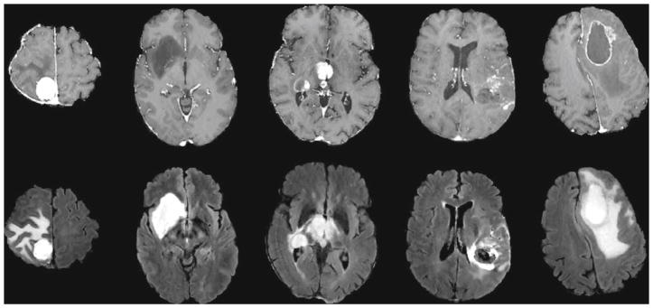
Examples of preprocessed axial T1 contrast-enhanced images (1st row) and FLAIR images (2nd row) with brain neoplasms. From left to right: meningioma, glioma grade II, III, IV, and metastasis

Attribute selection

The attribute selection is a widely known process, during which a subset of the most informative attributes is chosen, so that the highest accuracy is achieved using the least number of variables. Attribute selection involves searching through all possible combinations of attributes in the data to find which subset of them works best for prediction. To this end, the attribute selection algorithms are characterized by two components: (i) the method used to define the predictive value of each subset of attributes, denoted as feature evaluator, and (ii) the method determining the search over the attributes, denoted as search method.

In our study, three evaluators are used: a correlation-based feature selection (CFS) method [12], a method evaluating consistency in the class values [13], and an approach based on wrappers [14], as explained next. The CFS [12] algorithm evaluates the worth or merit of a subset of attributes by considering the individual predictive ability of each attribute along with the degree of redundancy between them. The equation below [15] formalizes the heuristic:

$${\text{Merit}}_s=\frac{k{\overline{r}}_{\text{cf}}}{\sqrt{k+k(k-1){\overline{r}}_{\text{ff}}}}$$

where Merit_s is the heuristic “merit” of a feature subset S containing k features, r̄_cf the average feature class correlation, and r̄_ff the average feature-to-feature intercorrelation. This equation is, in fact, Pearson’s correlation, where all variables have been standardized. The consistency measure [13] evaluates the predictive value of a subset of attributes by the level of consistency in the class values when the training instances are projected onto the subset of attributes. The consistency of any subset can never be lower than that of the full set of attributes. In the case of the wrapper approach [14], an induction learning algorithm is applied repeatedly on a distinct portion of the dataset using various feature subsets. A classifier is built on each feature subset using a set aside distinct portion of the dataset, and the feature subset with the highest performance (measured by some criterion) is used as the final set.

Also, in this study three search methods are examined, the Best First [16], Greedy Stepwise [17], and Scatter Search [18]. The Best First method [16] searches the space of attribute subsets by greedy hill climbing augmented with a backtracking facility. It starts with the empty set of attributes and searches forward. The Greedy Stepwise [17] method performs a greedy forward or backward search through the space of attribute subsets. It starts with a population of many significant and diverse subsets and stops when the accuracy is higher than a given threshold or there is no more improvement. Scatter Search [18] is an evolutionary method that combines solution vectors by linear combinations to produce new ones through successive generations.

Classification

In this study, several classifiers are examined: J48 tree [19], K-nearest neighbor (KNN) [20], VFI [21], SVMs [22], and Naïve Bayes [23]. J48 [19] is an implementation of C4.5 algorithm that produces decision trees from a set of labeled training data using the concept of information entropy. It examines the normalized information gain (difference in entropy) that results from choosing an attribute for splitting the data into smaller subsets. To make the decision, the attribute with the highest normalized information gain is used. The KNN algorithm [20] compares the test sample with the available training samples and finds the ones that are more similar (“nearest”) to it. When the k-nearest training samples are found, the class label in majority is assigned to the new sample. Learning in the VFI algorithm [21] is achieved by constructing feature intervals around each class for each attribute (basically discretization) on each feature dimension. Class counts are recorded for each interval on each attribute and classification is performed by a voting scheme. The Naïve Bayesian Classifier [23] assumes that features are independent. Given the observed feature values for an instance and the prior probabilities of classes, the a posteriori probability that an instance belongs to a class is estimated. The class prediction is the class with the highest estimated probability. The SVMs [22] first map the attribute vectors into a feature space (possibly with higher dimensions), either linearly or nonlinearly, according to the selected kernel function. Then, within this feature space, an optimized linear division is sought; i.e., a hyperplane is constructed which separates two classes (this can be extended to multiple classes).

Experiments

First, we examined all 10 pairwise problems between meningioma, glioma grade II, grade III, grade IV, and metastasis, using all the combinations of the above-mentioned methods. Examples of these tumor types are shown in Fig. 1. The purpose of this step is to choose the evaluators and the search methods, which provide high average accuracy, e.g., more than 90%. The multiclass problem is studied using the methods for attribute selection and classification that performed best in the pairwise classification problems.

Classification is performed by following a LOO strategy on the training samples.

Results

Pairwise classification

Table 1 shows the average accuracy (percentage of correctly classified samples) over all pairwise problems and the average area under the receiver operating characteristic curve (AUC), respectively, for the combinations that achieved accuracy greater than 90%. The results are sorted from the highest to lowest accuracy. It can be seen that the wrapper evaluator in combination with Best First and Greedy Stepwise search algorithms has the highest accuracy.

Table 1.

Average accuracy (ACC), AUC and number of retained attributes (N) over all pairwise classification problems

Evalutor	Search algorithm	Classifier	N	ACC (%)	AUC (%)
Wrapper	Greedy stepwise	VFI	5.1	96.6	95.1
Wrapper	Best first	VFI	5.1	96.6	95.1
Wrapper	Greedy stepwise	KNN (k = 3)	2.7	96.3	94.6
Wrapper	Best first	KNN (k = 3)	2.4	96.1	93.5
Wrapper	Best first	naive bayes	2.9	95.6	93.0
Wrapper	Best first	J48	2.4	94.4	91.8
Wrapper	Best first	KNN (k = 5)	2.2	94.3	90.8
Wrapper	Greedy stepwise	J48	1.8	92.7	85.3
Wrapper	Greedy stepwise	KNN (k = 5)	1.7	92.3	88.5
CFS	Best first	KNN (k = 5)	12	91.7	92.1
CFS	Greedy stepwise	KNN (k = 5)	11.7	91.0	92.1
CFS	Best first	KNN (k = 7)	12	90.8	91.2
CFS	Greedy stepwise	KNN (k = 7)	11.7	90.3	91.1
CFS	Scatter	KNN (k = 7)	11.4	90.2	92.8
CFS	Best first	KNN (k = 3)	12	90.1	91.1
CFS	Scatter	KNN (k = 5)	11.4	90.1	91.8

Among the pairwise problems the lowest accuracy (89.7%) is observed for the classification of gliomas grade II versus grade III and the highest accuracy (100%) for the classification of metastases versus meningiomas, metastasis versus gliomas grade II, meningiomas versus grade II or grade III or grade IV gliomas, and gliomas grade II versus gliomas grade IV.

Moreover, two additional pairwise problems were examined: primary neoplasms (gliomas) versus secondary neoplasms (metastases) and low versus high-grade gliomas. Meningiomas were not included in these combined classification problems because they differ from the glial tumors and metastases in both origin and behavior. The average LOO accuracy of the applied methods for these pairwise problems is displayed in Figs. 2 and 3, respectively. The wrapper evaluator in combination with the Best First search algorithm exhibits again the highest accuracy.

Fig. 2.

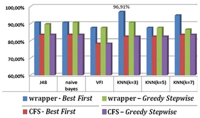
Average classification accuracy of primary neoplasms (gliomas) versus metastases

Fig. 3.

Average classification accuracy of low versus high-grade gliomas

When the presented attribute selection methods were used in combination with an SVM classifier, the results were similar or worse than those in previous work [9] using weighted SVMs [25]; however, the accuracy increased when a VFI or KNN (k = 3) classifier was applied instead of the SVMs. The good performance of the KNN classifier here might be attributed to the significantly small number of retained attributes, N = 2.4 and N = 2.7 on the average for all pairwise classification problems when the Best First and the Greedy Stepwise search algorithms were used, respectively.

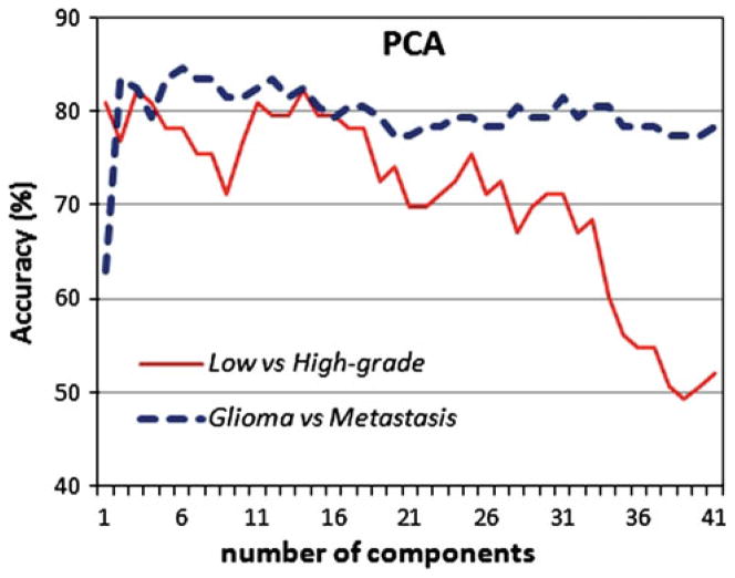
Finally, the proposed attribute selection method was compared against a popular dimensionality reduction method, the Principal Component Analysis (PCA) [26]. PCA, also named Karhunen–Loève transform, applies an orthogonal linear transformation that transforms the data to a new coordinate system of uncorrelated variables called principal components. The principal components are sorted such that the first components describe the direction of maximum variance of the data. We have applied PCA to reduce the number of variables and plotted the classification accuracy versus the number of retained components. As shown in Fig. 4, the classification accuracy is smaller than the accuracy of the proposed scheme for both classification problems, low versus high-grade gliomas and primary versus secondary neoplasms.

Fig. 4.

Attribute selection via PCA. The accuracy of a KNN (k = 3) classifier is shown versus the number of retained components for the classification of low versus high-grade gliomas and gliomas versus metastasis

Multiclass classification

The accuracy of LOO cross-validation of the multiclass problem is shown in Fig. 5. The highest accuracy (76.29%) is achieved when using the wrapper approach as evaluator, the Best First search algorithm and the VFI as classifier. The results in Fig. 5 illustrate that the wrapper approach outperforms the CFS evaluation method for the same classifier. The application of the Greedy Stepwise search method did not increase the accuracy.

Fig. 5.

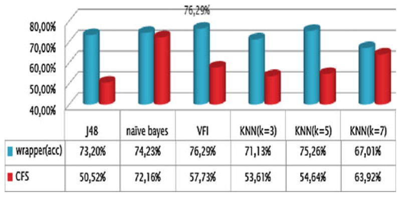
Accuracy for the multiclass problem

The confusion matrix for the best method is displayed in Table 2. Metastases get classified with very high sensitivity (95.8%) and glioblastomas and grade II gliomas with relatively high sensitivity (82.4 and 81.8% correspondingly). Grade III gliomas get classified with very low sensitivity; the largest portion is classified as grade II and the rest is assigned equally to GBMs and to metastases. The prediction of glioma grade is inherently difficult since brain neoplasms are often heterogeneous, meaning that different histopathologic features can be present throughout an individual neoplasm. The failure of the method to classify grade III gliomas possibly indicates that the extracted attributes do not form a separate cluster, but are rather similar to the attributes of the nearby classes (grade II and grade IV). The highest specificity is observed for grade III gliomas.

Table 2.

Confusion matrix for the multiclass problem

Metastasis	Grade2	Grade3	Grade4	← classified as
23	0	0	1	Metastasis
1	18	1	2	Grade2
3	6	5	3	Grade3
5	1	0	28	Grade4

For both pairwise and multiclass problems, the genetic algorithms and the neural networks were also investigated. However, the performance of the classification system did not improve.

Evaluation of attributes

The attributes of the final set are different for each classification pair and each attribute selection method. Table 3 shows the most frequently selected attributes over all pairwise problems. The 1st column shows the quantity being calculated, the 2nd column the MRI sequence exploited (when imaging characteristics are extracted), and the 3rd column shows the involved ROI. The most important attribute was the enhancing portion in T1 contrast-enhanced images; it was selected almost 3 times more often compared with the next most important attribute. This result is in accordance with other studies [9,27,28] and is justified by the fact that the presence of enhancing tumor is a decisive criterion in determining tumor malignancy during radiological diagnosis. Overall the attribute selection and ranking showed that parameters extracted from T1 contrast enhanced, FLAIR, and rCBV images were more informative than parameters from T1 and T2 images.

Table 3.

The most frequently selected attributes over all pairwise problems and the corresponding frequency (f)

Most frequently selected attributes characteristic	MRI	ROI*	f
Percentage enh. tumor	T1ce	1	55
Mean	T1ce	1 (margin)	20
Mean	T1ce	2 (central)	20
Variance	FLAIR	4 (margin)	13
Mean	FLAIR	4 (central)	13
Skewness	FLAIR	1 ∪ 2 ∪ 3	13
Circularity	–	1 ∪ 2 ∪ 3	13
Variance	FLAIR	4 (central)	12
Percentage necrosis	T1ce	3	12
Variance	rCBV	2 (central)	11
Irregularity	–	1 ∪ 2 ∪ 3	11
Percentage edema	FLAIR	4	10
Variance	T1ce	2 (central)	9
Mean	rCBV	1 (margin)	9
Variance	rCBV	4 (margin)	7

Attributes are extracted from ROIs (1 neoplastic enhancing, 2 neoplastic non-enhancing, 3 necrotic, 4 edematous)

Conclusions

In this study, several machine learning techniques for attribute selection and classification were examined with the purpose of brain tumor classification. The potential of attributes extracted from conventional and perfusion MRI was exploited and the diagnostic value of each attribute was investigated.

The highest accuracy was achieved by the wrapper evaluator in combination with the Best First search method for both the pairwise and the multiclass problems. The classifier achieving the highest accuracy was the KNN (k = 3) or the VFI depending on the classification problem, but the KNN is preferred due to its simplicity and overall more stable performance.

Concluding, the proposed classification scheme (consisting of the wrapper evaluator, Best First search method and KNN classifier) achieved overall high accuracy considering the fact that MR spectroscopy was not incorporated in the analysis. More extensive training using larger datasets is expected to further improve generalization ability of the scheme and also increase the performance of the whole classification system.

References

- 1.Prayson RA, Agamanolis DP, Cohen ML, Estes ML. Inter-observer reproducibility among neuropathologists and surgical pathologists in fibrillary astrocytoma grading. J Neurol Sci. 2000;175(1):33–39. doi: 10.1016/s0022-510x(00)00274-4. [DOI] [PubMed] [Google Scholar]
- 2.Tate AR, et al. Automated classification of short echo time in in vivo 1H brain tumor spectra: a multicenter study. Magn Reson Med. 2003;49(1):29–36. doi: 10.1002/mrm.10315. [DOI] [PubMed] [Google Scholar]
- 3.Majos C, et al. Brain tumor classification by proton MR spectroscopy: comparison of diagnostic accuracy at short and long TE. Am J Neuroradiol. 2004;25(10):1696–1704. [PMC free article] [PubMed] [Google Scholar]
- 4.Huang Y, Lisboa PJG, El-Deredy W. Tumour grading from magnetic resonance spectroscopy: a comparison of feature extraction with variable selection. Stat Med. 2003;22(1):147–164. doi: 10.1002/sim.1321. [DOI] [PubMed] [Google Scholar]
- 5.Lu C, Devos A, Suykens JAK, Arus C, Van Huffel S. Bagging linear sparse Bayesian learning models for variable selection in cancer diagnosis. IEEE Trans Inf Technol Med. 2007;11(3):338–346. doi: 10.1109/titb.2006.889702. [DOI] [PubMed] [Google Scholar]
- 6.Li G, Yang J, Ye C, Geng D. Degree prediction of malignancy in brain glioma using support vector machines. Comput Biol Med. 2006;36(3):313–325. doi: 10.1016/j.compbiomed.2004.11.003. [DOI] [PubMed] [Google Scholar]
- 7.Devos A, et al. The use of multivariate MR imaging intensities versus metabolic data from MR spectroscopic imaging for brain tumour classification. J Magn Reson. 2005;173(2):218–228. doi: 10.1016/j.jmr.2004.12.007. [DOI] [PubMed] [Google Scholar]
- 8.Rajendran P, Madheswaran M. An improved image mining technique for brain tumor classification using efficient classifier. Int J Comput Inf Secur. 2009;6(3) [Google Scholar]
- 9.Zacharaki EI, Wang S, Chawla S, Yoo DS, Wolf R, Melhem ER, Davatzikos C. Classification of brain tumor type and grade using MRI texture and shape in a machine learning scheme. Magn Reson Med. 2009;62:1609–1618. doi: 10.1002/mrm.22147. [DOI] [PMC free article] [PubMed] [Google Scholar]
- 10.Hall M, Frank E, Holmes G, Pfahringer B, Reutemann P, Witten IH. The WEKA data mining software: An update. SIGKDD Explor. 2009;11(1) [Google Scholar]
- 11.Liu H, Yu L. Towards integrating feature selection algorithm for classification and clustering. IEEE Trans Knowl Data Eng. 2005;17(4):491–502. [Google Scholar]
- 12.Hall MA. Correlation-based feature selection for discrete and numeric class machine learning. 17th international conference on machine learning (ICML); 2000. pp. 359–366. [Google Scholar]
- 13.Dash M, Liu H. Consistency-based search in feature selection. Artif Intell. 2003;151:155–176. [Google Scholar]
- 14.Kohavi R, John GH. Wrappers for feature subset selection. Artif Intell. 1997;97:273–324. [Google Scholar]
- 15.Ghiselli EE. Theory of psychological measurement. McGraw-Hill Book Co; New York: 1964. [Google Scholar]
- 16.Xu L, Yan P, Chang T. Best first strategy for feature selection. 9th international conference on pattern recognition; 1988. pp. 706–708. [Google Scholar]
- 17.Caruana R, Freitag D. Greedy attribute selection. 11th international conference on machine learning; 1994. pp. 28–36. [Google Scholar]
- 18.Laguna M, Mart R. Scatter search: methodology and implementations C. Kluwer; Dordrecht: 2003. [Google Scholar]
- 19.Gandhi GM, Srivatsa SK. Adaptive machine learning algorithm (AMLA) using J48 classifier for an NIDS environment. Adv Comput Sci Technol. 2010;3(3):291–304. [Google Scholar]
- 20.Cover TM, Hart PE. Nearest neighbor pattern classification. Inst Electr Electron Eng Trans Inf Theory. 1967;13:21–27. [Google Scholar]
- 21.Demiroz G, Guvenir A. Classification by voting feature intervals. 9th European conference on machine learning; 1997. pp. 85–92. [Google Scholar]
- 22.Chang C-C, Lin C-J. LIBSVM: a library for support vector machines. 2001 Software available at http://www.csie.ntu.edu.tw/~cjlin/libsvm.
- 23.John GH, Langley P. Estimating continuous distributions in bayesian classifiers. 11th conference on uncertainty in artificial intelligence; San Mateo. 1995. pp. 338–345. [Google Scholar]
- 24.Zacharaki EI, Wang S, Chawla S, Yoo DS, Wolf R, Melhem ER, Davatzikos C. MRI-based classification of brain tumor type and grade using SVM-RFE. 6th IEEE International Symposis Biomedical Imaging (ISBI 2009); Boston, Massachusetts, USA. 2009. [Google Scholar]
- 25.Huang Y-M, Du S-X. weighted support vector machine for classification with uneven training class sizes. Int Conf Mach Learn Cybern. 2005;7:4365–4369. [Google Scholar]
- 26.Jolliffe IT. Principal component analysis, series: springer series in statistics. 2. Springer; NY: 2002. [Google Scholar]
- 27.Al-Okaili RN, Krejza J, Woo JH, Wolf RL, O’Rourke DM, Judy KD, Poptani H, Melhem ER. Intraaxial brain masses: MR imaging–based diagnostic strategy—initial experience. Radiology. 2007;243:539–550. doi: 10.1148/radiol.2432060493. [DOI] [PubMed] [Google Scholar]
- 28.Lev MH, et al. Glial tumor grading and outcome prediction using dynamic spin-echo MR susceptibility mapping compared with conventional contrast-enhanced MR: confounding effect of elevated rCBV of oligodendrogliomas. Am J Neuroradiol. 2004;25(2):214–221. [PMC free article] [PubMed] [Google Scholar]