Abstract
In order to quantitatively analyze biological images and study underlying mechanisms of the cellular and subcellular processes, it is often required to track a large number of particles involved in these processes. Manual tracking can be performed by the biologists, but the workload is very heavy. In this paper, we present an automatic particle tracking method for analyzing an essential subcellular process, namely clathrin mediated endocytosis. The framework of the tracking method is an extension of the classical multiple hypothesis tracking (MHT), and it is designed to manage trajectories, solve data association problems, and handle pseudo-splitting/merging events. In the extended MHT framework, particle tracking becomes evaluating two types of hypotheses. The first one is the trajectory-related hypothesis, to test whether a recovered trajectory is correct, and the second one is the observation-related hypothesis, to test whether an observation from an image belongs to a real particle. Here, an observation refers to a detected particle and its feature vector. To detect the particles in 2D fluorescence images taken using total internal reflection microscopy, the images are segmented into regions, and the features of the particles are obtained by fitting Gaussian mixture models into each of the image regions. Specific models are developed according to the properties of the particles. The proposed tracking method is demonstrated on synthetic data under different scenarios and applied to real data.
Index Terms: Particle tracking, multiple hypothesis, clathrin mediated endocytosis, fluorescence microscopy
I. Introduction
With the rapid development in fluorescence microscopy, biologists can observe the dynamics of individual particles and investigate the molecular mechanisms underlying the cellular and subcellular processes. Total Internal Reflection Fluorescence (TIRF) microscopy [1], in particular, allows observing events that occur near the cell cortex such as endocytosis, exocytosis and the associated remodeling of the surrounding cytoskeleton. Studies of these processes can lead to better mechanistic understanding of related diseases. We are particularly interested in clathrin mediated endocytosis (CME) [2]–[4], an essential subcellular process. CME has house-keeping functions in almost all types of cells. It is used to take up nutrients and other extracellular material, to internalize plasma membrane proteins such as receptors and transporters, and to compensate the increase in surface area resulting from fusion of secretory vesicles with the plasma membrane. CME also plays specialized functions in specific cell types. For instance, CME is a major route for synaptic vesicle recycling at neuronal synapses, a process essential for synaptic transmission [2], [5], and dysfunction of the process may be implicated in several neurological and psychiatric diseases including Alzheimer disease [6]–[8]. Abnormal function of CME can be involved in cancer [9] and diabetes [10]. Also, CME is one of the pathways through which viruses enter cells [11].
The CME process [2] is illustrated in Fig. 1: Adapter binds to cell plasma membrane and recruits clathrin, a type of protein. The outer layer of a particle is assembled from clathrin, which is called clathrin-coat. A small portion of the cell membrane invaginates to form the inner layer of the particle. Then the particle matures and remains stable for a while. In the final stage, the neck of the particle, which links to the cell membrane, is cut off, which is called fission, and then the clathrin coat is dissociated, which is called uncoating. The entire process can be monitored by fluorescence microscopy if a component of the clathrin coat is labeled with a fluorescent tag in the living cell. The particle is called clathrin coated pit (CCP) before fission, and after fission it is renamed as clathrin coated vesicle (CCV) until uncoating. For the sake of simplicity, we call it as CCP particle in the rest of this paper. During the process, the fluorescence intensity of the particle increases as new clathrin comes, and remains at a relatively stable level after the particle matures, and then decreases rapidly after fission due to dissociation/shedding of clathrin units (uncoating) and exiting from the TIRF illumination field. The movement of each particle is mainly caused and constrained by two factors. First, tiny molecules in cytosol randomly hit each particle during the whole process. Second, the neck of each particle prevents it from going far away from its connection point on the cell membrane.
Fig. 1.

(a) A TIRF image of a cell expressing GFP- clathrin light chain shows CCP particles. Fluorescence appears white, and each bright spot represents a particle. (b) Cartoons and a real image sequence (smoothed) show different stages of CME. The three-legged structures of pinwheel shape represent clathrin (blue color). The red dots indicate center positions and the green lines represent trajectories. The particle has a neck connected to cell membrane until fission.
For quantitative studies of CME, biological parameters need to be calculated from the features of the CCP particles. However, since image datasets from an experiment typically consist of several thousand image frames, manual processing is very painful. Due to the importance and complexity of CME, it is very useful to develop an automatic tracking method.
To design a particle tracking method, there are two major challenges. The first one is to design appropriate models according to the properties of the particles. Different types of particles may look similar but have significantly different dynamics (e.g., different types of motions). In the literature, particle appearance models [12] are well studied, e.g., Gaussian model, and directly applicable to many applications, but different dynamic/motion models need to be designed for different types of particles. There are many particle tracking methods for different biological applications [13]–[19]. For example, in [18] a method is proposed to track microtubule tips moving at nearly constant velocity, which can be well described by a linear motion model. In [13], a method is presented to track quantum dots which can rapidly switch between acceleration mode and steady speed mode. Equipped with multiple motion models and an interacting multiple model (IMM) filter, that method [13] is able to track the targets with the switching modes. The properties of the CCP particles are different from those of the other particles: CCP motion is constrained as compared to the relatively free motions of the others; new CCP particles can appear near the positions where matured CCP particles disappear, and as a result, independent trajectories may be erroneously linked together without using proper models. Therefore, those methods are not directly applicable for our application.
The second challenge is to manage trajectories and handle data associations effectively when the number of particles is large, which requires good tracking frameworks. A particle tracking method can be as simple as tracking each particle independently by calculating image correlations [20], but it can not handle complex scenarios. To track multiple particles together, most of the particle tracking methods in the literature consider tracking as statistical inference with different criteria such as MAP (maximum a posteriori) and MMSE (minimum mean squared error) [20]–[23], and try to solve it in various ways. Some methods use stochastic sampling based frameworks [24], e.g., particle filter [18], [25] or Markov chain Monte Carlo (MCMC) [26]–[28], to numerically approximate the posterior probability function by a set of weighted samples when the tracking problem is nonlinear and non-Gaussian. The nonlinearity is mainly induced in the imaging process, in which the observed bright spots are the results of convolutions between the optical system function and the fluorophore distributions of the particles. The non-Gaussian property mainly arises from image noises, e.g., photon shot noise in CCD cameras, which follows Poisson distribution. The motion of the particles can always be modeled using linear models, even when the type of the motion is nonlinear, and therefore, its contribution to nonlinearity can be ignored. Similarly, image noise distributions can be well approximated by Gaussian distributions when image signal is high enough [29], [30]. Based on those properties, many other methods tailor the classical multiple hypothesis tracking (MHT) method [31] to fit into different applications [13], [19], [23], [32], [33], in which particle detection is separated from the other tasks as an independent module and stochastic sampling is no longer needed.
In the MHT framework [24], target (e.g., particle) tracking can be decomposed into three tasks: detection, state estimation and prediction, and linking. Detection is to find the positions of the targets and estimate some other features in a single image, i.e., at each time. By assembling these estimated features of a target into a vector at each time, we get the observation/measurement of the target at each time. State estimation is to recover some features that are not directly observable in a single image (e.g., intensity variation), or refine some features that contain noises (e.g., intensity). By assembling all the features of a target into a vector at each time, we get the state vector of the target at each time. State prediction is to predict the state of a target in the near future based on current and past information. Filters may be used for state estimation and prediction, such as Kalman filter if only one linear model is used, or interactive multiple model (IMM) filter if multiple linear models are used. Linking is to find the most probable trajectories by considering the observations from multiple image frames. In another point of view, linking is to find the correspondences between the trajectory tags and the observations which is the so-called data association problem. Therefore, linking is just a combinatorial optimization problem, and can be solved by using a variety of algorithms [23], [34]–[37]: graph based algorithms, or dynamic programming, or integer programming. The objective functions used in the linking task are related to particle models, observations, estimated states and predicted states. The MHT framework is more straightforward compared to the stochastic sampling based approach, and tracking results are strictly reproducible which is required in our application.
The known issue of the MHT framework is the solution space will expand exponentially fast as the number of image frames used for linking increases, which may require an unaffordable amount of computer memory. Many methods are proposed to overcome the issue. The most straightforward and effective one [34] is to use a sliding time window to restrict the number of image frames used for linking. Since computer memory and CPU speed have significantly increased in recent years, methods based on MHT and sliding time window have become practical in real biological applications [23], [32].
The MHT framework has an implicit assumption that the observations of the targets are already given by the detection module except that it is not known which observation corresponds to which target, and vice versa. The assumption can be violated in two situations as explained in the following two paragraphs.
Firstly, if the images have very low signal to noise ratios (SNRs), e.g., SNR = 1, then the signals of the particles will be buried in the background noise and almost cannot be detected. In our application, when a CCP particle is at the very beginning of the assembly stage or at the very end of the uncoating stage, its signal is below the detection limit and therefore can not be detected, but that does not matter as long as we can observe its majority activities. Since TIRF microscopy is used in our application, image SNR is relative high (much higher than 4 usually), and therefore this situation is not our concern.
Secondly, if particle density is high, then pseudo- splitting and merging events will occur frequently. The size of each particle is usually smaller than the spatial resolution of the microscopy. As a result, if particles come too close to each other, they can not be distinguished clearly. In extreme cases, some particles actually move very close to each other at some time t such that the local intensity profile can be well described by a single Gaussian function. Although it looks like a merging event happens, particles do not merge physically. Due to such events, detection may be imperfect, that is, there are no strict correspondences between observations (i.e., detected particles) and particles (i.e., real particles). For example, two observations in an image region may be related to three particles or more. In our application, some CCP particles may temporarily crowd together (pseudo-merging) and then move apart (pseudo-splitting). As a result, there may be many suspicious observations, each of which may correspond to several particles, and the number of corresponding real particles and their states are all unknowns. To solve this kind of problem, a direct approach is to fit more than one Gaussian function around every suspicious observation. Since the number of particles corresponding to each suspicious observation is unknown, the optimal number of Gaussian functions to be fitted is also unknown. As a result, either the total number of particles needs to be known or fixed which is unrealistic, or some thresholds [38] need to be specified by the user, but it is difficult to find good thresholds manually. There are some indirect approaches worth trying such as pixel clustering [39] and finite mixture model learning [40]. A method in [41] uses k-means based functions to cut the suspicious observations into pieces, and find the best result. That concept is not applicable for our application because when more than one particles move close, the local intensity profile will be a mixture of Gaussian functions intersecting with each other, and small segments of the profile are meaningless. By considering the image intensity profile as the joint probability distribution function of spatial points, finite Gaussian mixture model learning is another candidate method [40]. However, when the particles are very close, the local intensity profile tends to be unimodal, and as a result, the exact number of the particles can not be extracted by that method. If some prior information of the particles in the local regions, including their number, is provided, the direct approach of Gaussian function fitting [38] can work well, no matter how close the particles are. If we analyze not only the image at time t but also before and after time t, we will get additional information to guide the Gaussian function fitting process at time t, and then it will be easy to tell that some particles come to the same region and then move apart. The key idea is to integrate information from trajectories, observations, and images all together, which will be used in the proposed method.
This paper is an extension of our previous works [42]–[44]. It presents a multiple hypothesis based particle tracking framework, and describes how to model CCP properties, and shows how to apply the tracking framework with the models. Compared to our previous papers, here we present many new enhancements which make the tracking method robust and efficient, and provide more validation results. The key idea of our tracking method is to generate and evaluate many observation candidates and trajectory candidates, and only keep the best subset of them as the tracking result. To generate the candidates, an exhaustive search based method is straightforward and easy to be implemented, as we did previously, but it requires a long processing time which is undesired by the users, i.e., the biologists. In this paper, we present new candidate generation algorithms which can significantly reduce the search space. We also present a strategy to automatically determine the parameters of the state models, which previously are obtained by analyzing manually tracked trajectories. We test the method extensively in simulation with different particle densities and signal to noise ratios. We also test the method on image datasets from real biological experiments, which consist of images from not only normal cells but also altered cells, and provide more information about the biological application.
The remainder of the paper is organized as follows. In section II, we introduce the tracking framework which is an extension of the classical MHT framework, and allows different types of hypotheses. It has the build-in capability to handle the pseudo- splitting/merging events effectively without user intervention, and prevent independent trajectories from linking together. In section III, we describe the CCP models including dynamic state models and appearance models, provide the detection method, describe the method for multiple candidate generation, and discuss some implementation issues. In section IV, we show the evaluation results on synthetic data and real data. We conclude this paper in section V.
II. Tracking Framework
In this section, we present the particle tracking framework. We first show the classical MHT framework, and then present the extensions. We call the extended framework as E-MHT.
We make the following notations. Let It be the image acquired at time t (frame index), which can be a 2D image or a 3D image volume. Let Xt be the set of the states of all the targets (i.e., particles) at time t, assembled from each target's state , i.e., and k is the index (i.e., unique identifier) of a target and its trajectory. Let Dt be the set of all the observations at time t, assembled from each observation , i.e., , and j is the index of an observation at time t. Each observation also has a global index (i.e., unique identifier) l. Let Let denote the observation that corresponds to the target k at time t. For the sake of convenience, the two words, particle and target, are used interchangeably in this section.
A. The MHT Framework
The goal is to find the target states that maximize the posterior probability (MAP) given the image dataset , i.e., maximize the energy E:
| (1) |
Here, . Since it is difficult to find the optimal solution directly, we try to maximize the lower bound Ê of the above energy (the proof is in the appendix). Assuming the targets are statistically independent of each other and applying Bayes' rule, then we obtain
| (2) |
| (3) |
| (4) |
Each trajectory is a candidate and has an indicator α(k) ∈ {0, 1}. If α(k) = 1, the trajectory candidate k is selected as a true trajectory, and if α(k) = 0, it is discarded as a false trajectory. By considering different correspondences between the targets and the observations, multiple trajectory candidates can be generated. One to one correspondences between trajectories and observations are assumed, which is the constraint of the maximization problem.
If we only use the above equations as the framework, then it will just be equivalent to the classical MHT. We further extend the framework as described in the following subsections.
B. Multiple Observation Candidate Generation
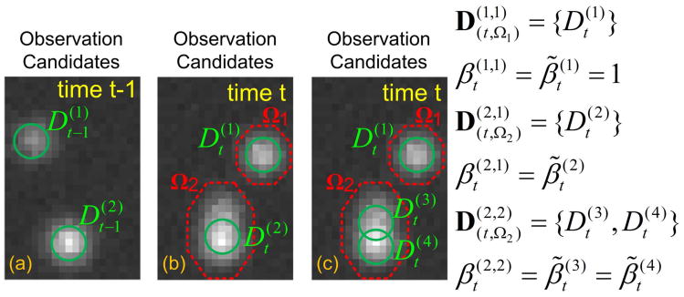
Not only multiple trajectory candidates but also multiple observation candidates are generated. In most cases, each image It can be segmented into small regions . Each sub-image I(t, Ωm) many contain one or more observations. In each image region Ωm, we try to generate many observation-sets, and each of them indexed by n, can explain the sub-image I(t, Ωm) independently. Then, we extend Eq.(4) to
| (5) |
| (6) |
| (7) |
Each observation is a candidate and has an indicator . If , the observation is selected as being true, and if , then it is rejected as a false one. Each observation-set also has an indicator . If , the observation-set is selected, and if , then it is rejected. Since the individual observations in each observation-set should be true or false all together, then the indicator of an observation-set is equal to the indicator of each observation in the set. If there is only one observation in the set, then the indicator is 1. For CCP tracking, Eq.(6) will be defined in section III-B.
The method for generating good observation-sets is not defined here, we leave it to be implemented in different applications using different strategies. By generating multiple observation candidates and finding the best candidates, the number of particles in each segmented region can be determined. Fig. 2 shows the observation candidates generated in a simple scenario, and Fig. 3 shows the relations among the indicators.
Fig. 2.
(a) Two observation candidates at time t−1. (b) Two observation candidates at time t. (c) Three observation candidates at time t. By linking the observation candidates between image frames with different combinations, we can get many trajectory candidates.
Fig. 3.
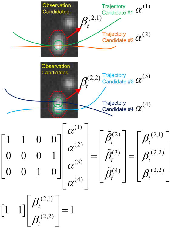
The relations among the indicators.
C. Solving the Optimization Problem
After obtaining the candidates of trajectories and observations, the only task left is to find a set of candidates as a solution that is feasible and maximizes the energy in Eq.(2). In a feasible solution, there must not exist any observation which is shared by more than one trajectory, and there must not exist any pair of observation-sets, each of which explains the same image region. The feasibility constraint on the solution ensures one to one correspondences between the selected trajectories and the selected observations at each time. Eq.(2) and its constraints can be rewritten to the matrix forms, given by
| (8) |
| (9) |
| (10) |
After integer programming is applied, the binary vector γ is obtained as the solution. γ is defined as γ = [α′, β′]′. Here ′ is vector transpose operator, and all the vectors in this paper are column-shaped. α and β are two binary vectors assembled from every unknown α(k) and every unknown respectively.
In Eq.(8), E is a vector assembled from all the corresponding and . In Eq.(9), β̃ is a vector assembled from every individual observation indicator . A is a sparse binary matrix. If the trajectory candidate k passes the observation candidate indexed by l, then A (l, k) = 1. The summation of the indicators of the trajectories that have the same observation (e.g., the one indexed by l) is equal to the indicator of that observation, which is the one-to-one mapping constraint described by Eq.(9). In Eq.(10), B is a sparse binary matrix, and 1 is a vector and all its elements are equal to 1. Eq.(10) is just the matrix form of Eq.(7). Examples of Eq.(9)&(10) are given in Fig. 3. In the implementation, only one set of binary variables is needed to represent the two types of observation indicators and .
Here, the trajectory-related hypothesis is whether a recovered trajectory is a real one, and the observation-related hypothesis is whether an observation belongs to a real particle, which is the reason the method is called multiple hypothesis based. Compared to the classical MHT framework, the extended MHT framework tests not only multiple trajectory-related hypotheses but also multiple observation-related hypotheses.
III. Applying the Framework for Tracking CCP Particles
To use the tracking framework, we need to model the properties of the CCP Particles, design particle detection methods and candidate generation methods, and define relevant energy terms. The energy is related to the dynamic models (i.e., state space models), and the energy is related to the appearance model. Since in most biological experiments only 2D imaging is performed, we restrict our discussion in 2D throughout the rest of the paper, although 3D extension is straightforward. For the sake of convenience, the two words, particle and target, are used interchangeably in this section.
A. State Space Models and Filters
We assume particle dynamics can be modeled using linear state space models [45], [46] with a certain probability distribution at each time. π(i1, i2) is the model transition probability for each particle to switch from mode (model) i1 to i2 when the current mode (model) is i1, and Σi2 π(i1, i2) = 1. Each model i has a posterior probability for each particle k, and . Each model is given as
| (11) |
| (12) |
Here, F(k) is the state transition matrix. is the external input that we use to impose constraints. W(i) is the process noise with covariance matrix Q(i) estimated from training data. H is a constant observation matrix. is the observation noise with covariance matrix provided by the detection module. Each of these noise sources is assumed to be Gaussian and independent.
We define the state of each particle k at time t as . is its position. is its intensity, and is the rate of intensity change over time. is its relative radius. We propose to use two linear state space models. For particle motion, the first model describes it as free Brownian motion because the motion is indeed random, and the second model describes it as confined motion because each particle is linked to the cell plasma membrane through its neck and can only move within a restricted region before fission [2]. For intensity variation of each particle, both models describe it as a linear process.
The matrices are given by
is a zero vector, and is related to the force that keeps the particle staying near the connection point on cell membrane (see Fig. 1) which is estimated to be the time-average position , and t1 is the starting-time of the trajectory. And, let t2 be the ending-time of the trajectory, then the lifetime of the particle is t2 − t1 + 1.
In Eq.(3) the lifetime of each particle is extended to be equal to the number of images, which is a common trick [47] to deal with target appearing and disappearing. Since the process is assumed to be Markovian, we obtain
| (13) |
To deal with particle appearing and disappearing, we set and according to particle properties. Δ is the maximum particle displacement. aap is the average intensity of the particles shortly after they appear. adp is the average intensity of the particles shortly before they disappear. Those parameters can be learned from training data. We define for t < t1 − 1, and for t > t2 + 1, which means the states are irrelevant before the particle is created and after it disappears.
To simplify the computation of the energy , we make several approximations. In the right side of Eq.(3), the second term can be ignored because observation noise level is much smaller than process noise level in our application. The element in Eq.(13) can be approximated as
| (14) |
is the estimated state given the observations up to time t. is the predicted state given the observations up to time t − 1. Q̂(i*) = HQ(i*)H′ where i* is the index of the most probable model at time t. The vector norm is defined as . We insert the H matrix in the norm to ensure that only observable features are used to evaluate the goodness of each trajectory.
For state estimation and prediction, we use the well known IMM filter [13], [23], [46], [48]. For the details of the filter we refer the reader to [46], [48]. In addition, the feasible region of the predicted observation of a particle is also estimated, which is realized by using the gating technique [23].
For model parameter estimation, labeled training data is preferred if it is available. However, since in real situations cell to cell variation is large, it is risky to use the parameters trained on previous labeled data for new data. Instead, parameters are estimated in an iterative fashion similar to the approach in [49], directly from the datasets to be analyzed: After the tracking algorithm is performed on the selected regions, parameters can be estimated from the recovered trajectories; then with the estimated parameters, tracking is performed to update the trajectories. In our application, two iterations are sufficient, and the image regions with high particle density (e.g., around cell center) are excluded before parameter estimation. In experiments, the model transition probability is set as π(1, 1) = 0.8, π(1, 2) = 0.2, π(2,1) = 0.2, π(2,2) = 0.8 for all cases. The observation noise covariance matrix is assumed to be a diagonal matrix, and each component/variance is estimated from the performance curves of the detection method obtained from simulation [43].
B. Appearance Model
To observe the particles, proteins of interest are fluorescently labeled. Particle diameter is comparable to the lateral pixel size, and the light from each particle is blurred by point spread function (PSF). As a result, the spatial distribution of the fluorescence intensities of a single particle in the xy-plane can be well modeled using a Gaussian function, which is widely studied in the literature [12], [50]. The fluorescence lights emitted from individual particles are captured by CCD camera. EM-CCD [29], [30] is widely used in high performance microscopes because it can detect light with very low intensity and almost eliminate readout noise.
Therefore, before it is captured by the camera, the 2D fluorescence signal ft(x, y) can be modeled as the sum of Gaussian mixture Gt(x, y) and background bt(x, y), given by
| (15) |
The Gaussian mixture Gt(x, y) has multiple components, i.e., . Each component corresponds to a feature/observation vector , given by
| (16) |
The image It(x, y) from the EMCCD camera is determined by the input fluorescence signal ft(x, y) and the noise sources [30]. We can approximate it as
| (17) |
| (18) |
Nt is zero-mean Gaussian noise with variance . The approximation in Eq.(17) is only used for feature estimation not for simulation. Let's assume we have obtained an observation-set in the region Ωm. Then we can calculate the energy term in Eq.(6) by using Eq.(18) and restricting (x, y) in the region.
C. Initial Particle Detection
We have developed a particle detection method [43]. Initial positions of the particles are identified in each image by using Laplacian of Gaussian (LoG) based filters. Then, image background is estimated and Gaussian mixture models are fitted to obtain the full observation vectors. For the details we refer the reader to [43]. Since the sizes of the CCP particles do not differ much and the background is almost homogeneous, and therefore the image filter based detection method is appropriate for our application [12]. We further extend the method to segment each image into regions containing particles by thresholding the filtered images. In the resulting binary images, the skeleton of each region [51] is calculated and will be used for generating observation candidates. Fig. 4 shows the detection result on a real image region.
Fig. 4.

Particle detection and image segmentation result. (a) 6 observations of particles indicated by green circles. (b) 5 segmented regions. (c) The skeletons of the regions.
D. Multiple Candidate Generation
The initial observations are obtained by using the method in section III-C. Once temporal information is available, in every image region, we try to generate multiple observation candidates. Let's suppose that target trajectory candidates up to time t − 1 have been obtained. In the image It, each segmented region Ωm intersects the predicted observation regions of some targets/particles {X(k1), X(k2), …} which is called the feasible target set. If the set has more than one targets, then we start to generate multiple observation candidates in the region Ωm.
There are two possible approaches to generate observation candidates with temporal information. The first approach is to fit Gaussian functions to the image region with different numbers. The second approach is to treat the image intensity as spatial probability distribution at each pixel, and fit probabilistic Gaussian mixture models in the image region. The second approach usually uses expectation-maximization (EM) style algorithms to do optimization, and it is relatively slow compared to the first approach. Therefore we use the first approach.
For each subset {X(kh1), X(kh2), …} of the feasible target set, if these targets do not conflict with each other, i.e., not sharing the same observation in each of the past image frames, then we find their optimal observation-set which maximizes the energy:
| (19) |
subject to (for each kh)
| (20) |
| (21) |
The first term in Eq.(19) is just calculated by using Eq.(18) and considering the pixels only in the region. The second term in Eq.(19) ensures that each estimated intensity will be close to its predicted value . Eq.(20) assumes that each radius almost does not change in a short time, i.e., equal to its predicted value . Eq.(21) ensures that each estimated position is located within a circle centered at its predicted position .
For each subset in which the targets do not conflict with each other, we find its optimal observation-set . We may get more observation candidates by keeping more than one suboptimal observation-set. For our application, the optimal observation-set is sufficient.
The candidate generation process starts with 2-element subsets of the feasible targets, and then subsets with more elements are considered. If we use exhaustive search based methods to generate candidates, the number of candidates will go up exponentially fast, but most of them will be rejected later, which is a waste of time and computation. To reduce the search space and speed up the computation, firstly, the x-y positions of the observations are restricted to be on the skeleton and the local intensity maxima of each region, and the coarse estimation is obtained. And then each observation is allowed to vary within 1 pixel to get refined result. The rationale is the observations are located with high probability on the local maxima or the skeletons. To control the process, if the energy decreases when the number of elements in the subset increases, then the process stops. The details are described in Algorithm 1.
Generating trajectory candidates is relatively straightforward, and we use four types of trajectory candidates. Let's assume that target trajectory candidates up to time t − 1 and observation candidates at time t have been obtained. A target trajectory is extended if an observation is feasible (i.e. within the predicted range) for the target. A target trajectory is terminated if there is no feasible observation for the target, or if all the feasible observations of the target are also feasible for some other targets. A candidate of new trajectory starting with an observation is created if the observation is infeasible for every target, or if the observation is feasible for some target which has other feasible observations. New candidates are also created by breaking a terminated target trajectory into several parts, if the smoothed time-intensity curve of the trajectory has some local minima that are not located at the beginning or the end. The breaking points are located at these local minima. The last type of candidates are used to prevent independent trajectories from jointing together, which is not considered in the classical MHT.
|
|
| Algorithm 1 Observation Candidate Generation in a Region |
|
|
| Input: |
| Ωm: the image region |
| Sm: the set of positions on the skeleton of the region |
| Pm: the set of positions of the local maxima in the region {X(k1), X(k2), …, X(kN)}: the set of feasible targets |
| Start: |
| n = l |
| Emax = 0 |
| For i = 2 to N |
| k = 0 |
| Step 1: try to get a new subset {X(kh1), X(kh2), …, X(khi) |
| If a new subset is available, then go to Step 2 |
| Else, go to Step 5 |
| Step 2: check the subset |
| If the subset is feasible, then go to Step 3 |
| Else, go to Step 1 |
| Step 3: n = n + 1, find the observation-set , which maximizes Eq.(19) |
| (1) Search on Sm and Pm to get initial result |
| (2) Alow the observations to vary within 1 pixel, get refined result and the energy |
| Step 4: check the observation-set |
| If , then keep it and k = k + 1 |
| Else, discard the observation-set and n = n − 1 |
| Go to Step 1 |
| Step 5: If k > 0, then Else, break the For loop |
| End |
| Output: |
| observation-sets and associated subsets of the targets |
|
|
E. Implementation of the Tracking System
The tracking system is illustrated in Fig. 5. It consists of a detection module, a trajectory module, and a decision module. The detection module generates observation candidates as described in section III-C and III-D. The trajectory module generates trajectory candidates and estimates the states of the particles. The decision module evaluates all the candidates by calculating the energy terms in Eq.(2) and selects the best set of candidates by solving the integer programing problem Eq.(8)–Eq.(10). After the initial detection results on all the images are obtained by using the detection module, the other two modules start. Once the tracking is finished, the order of the image sequence is reversed and the tracking system runs again to provide the final result. As the reader may notice, it is not mentioned how to solve the pseudo-splitting problem in section III-D. However, by tracking in the backward time direction, the problem can be solved, because a splitting event in the forward timeline is equivalent to a merging event in the reversed timeline.
Fig. 5.
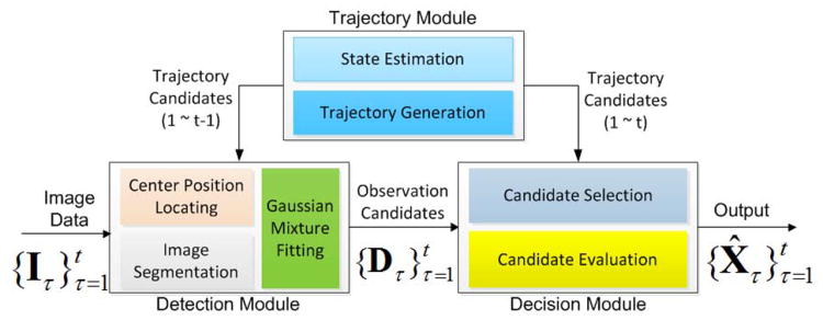
The diagram of the tracking system.
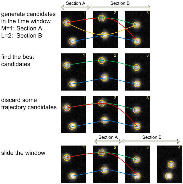
To make the tracking process efficient, we use the sliding time window technique as shown in Fig. 6. Let's assume we have a set of candidates generated in a window with length L ending at time t. The window slides with M steps (M < L), and new candidates are generated. Then, all the candidates generated in the interval [t − L + 1, t + M] are evaluated, i.e., performing integer programming to find the optimal candidates. If the window has not reached the end of the image sequence, only the candidates in the interval [t − L + 1, t − L + M] that conflict with the optimal candidates, will be discarded. If the window reaches or exceeds the end of the image sequence, only the optimal candidates will be kept.
Fig. 6.
An example to show the sliding time window technique.
IV. Experimental Results of CCP Tracking
A. Evaluation on Synthetic Data
The proposed method is evaluated using simulation with different signal to noise ratios (SNRs) and particle densities. The models in section III-A are not used in simulation because they are just linear approximations. Instead, a set of CCP trajectories are obtained from very low particle-density regions of real image data, and confirmed by expert biologists. In order to control SNRs, these trajectories are adjusted by smoothing and rescaling their time-intensity curves. To simulate a trajectory, one trajectory record is randomly chosen from that set, and then it is randomly placed on the image planes. Images are simulated by following the TIRF imaging theory [1], [52], [53], similar to the previous works [54], [55] in our group. Two major types of noises are considered in the simulation process: the Poisson (shot) noise of input photon and the excess noise generated in the EMCCD. The SNR of each dataset is defined as the average SNR of individual particles in the dataset. By varying the background noise level, the SNR of each dataset can be tuned in a large range. Since, in real images, particle density is very high around cell center and very low near cell boundary, in simulation we choose four particle densities: 0.005/pixel2, 0.006/pixel2, 0.007/pixel2, and 0.008/pixel2 to represent the densities of different regions.
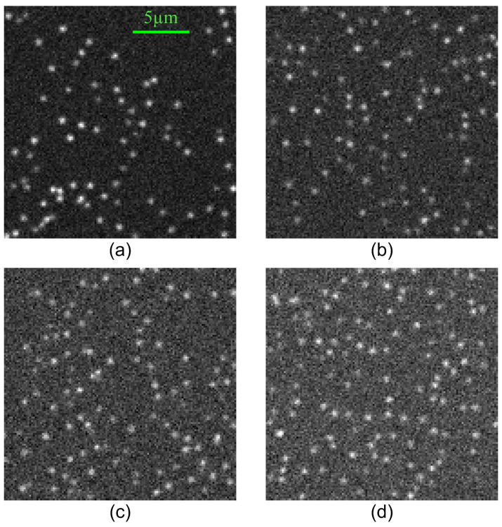
We first create noise-free datasets with different particle densities, and then we add noises at different levels to the noise-free datasets to create the final datasets. Each dataset contains 200 image frames, and the size of each image is 128 × 128 pixels (1 pixel=160nm). Particle appearing and disappearing occur almost on every frame. Examples of simulated images are shown in Fig. 7. The feature estimation accuracies of the detection module have been reported in [43] and [55]. The absolute position estimation accuracy is not very important in our application as long as the localization error is within one pixel which has been achieved by the detection module. Here, we focus on evaluating the overall performance of the tracking method.
Fig. 7.
Examples of synthetic images (128 × 128 pixel, and 1 pixel = 160 nm): (a) Density = 0.005/pixel2 and SNR = 8. (b) Density = 0.006/pixel2 and SNR = 6. (c) Density = 0.007/pixel2 and SNR = 5. (d) Density = 0.008/pixel2 and SNR = 5.
To measure tracking performance, we use Jaccard similarity to measure the goodness of the tracking result on each dataset. It is a general measurement of detection and data association accuracy, given by
| (22) |
Before the calculations, the best correspondences between the recovered trajectories and the ground truth trajectories are found by using the method in [56]. The recovered trajectories refer to the trajectories produced by a tracking algorithm. The ground truth trajectories are just the simulated trajectories. The distance threshold of matching is set to be 3 pixels, which means if the distance between two positions in two trajectories (recovered vs. ground truth) is greater than the threshold, then the two positions do not match each other. If a position (e.g., ) in a recovered trajectory corresponds to a position (e.g., ) in a ground truth trajectory, then there is a matched position in the recovered trajectory. If a position in a recovered trajectory does not correspond to any position in the ground truth trajectories, then there is an unmatched position in the recovered trajectory. If a position in a ground truth trajectory does not correspond to any position in the recovered trajectories, then there is an unmatched position in the ground truth trajectory. T P (true positive) is the number of matched positions in the recovered trajectories, and F P (false positive) is the number of unmatched positions in the recovered trajectories. F N (false negative) is the number of unmatched positions in the ground truth trajectories.
In order to calculate bio-parameters in our application, e.g., lifetime, the tracking result should contain less false trajectories and more correctly recovered trajectories, and cover the ground truth trajectories as many as possible. Therefore, Jaccard similarity is the most relevant metric for our application. In fact, Jaccard similarity is not only a general measurement of tracking accuracy, but also an approximation of the lifetime estimation accuracy:
| (23) |
Here, LT means lifetime, and GT means ground truth. If a trajectory starts at time t1 (image index) and ends at time t2, then its lifetime is t2 − t1 + 1, or (t2 −t1 + 1) × sampling interval. If the number of unmatched positions in a recovered trajectory is equal to its lifetime, then it is a false trajectory.
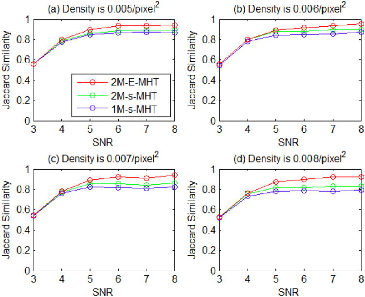
To evaluate the proposed method, we may compare it to some tracking methods in the literature. However, since different models and detection methods are used in different tracking methods for different applications, direct comparisons are very difficult and unfair. Instead, we choose three representative MHT-based methods [13], [19], [23] and equip them with the detection method described in section III-C, and particle models related to our application. The first method is based on the one in [19], and we equip it with the Brownian motion model, and we name it as 1M-s-MHT where 1M refers to the Brownian motion model, and s means simplified because it uses frame-by-frame linking. The second method is based on the one in [13], and we equip it with the CCP state models and the IMM filter described in section III-A, and we name it as 2M-s-MHT where 2M refers to the two CCP state models and s also means simplified for the same reason. The third method is based on the one in [23] which uses the same type of sliding time window, and we equip it with the CCP state models and the IMM filter, and name it as 2M-MHT. We call the proposed method as 2M-E-MHT where E means extended.
The performance curves of the methods, 2M-E-MHT, 2M-s-MHT and 1M-s-MHT, are shown in Fig. 8. To make a fair comparison, we set the size of the sliding time window in the proposed method as L = 2 and M = 1. Since the method 1M-s-MHT uses the least amount of information, it has the lowest performance. By using the CCP state models, the method 2M-s-MHT does better than the method 1M-s-MHT in some scenarios. By applying the extended MHT framework with the CCP state models, the proposed method 2M-E-MHT performs consistently better than the other two methods. As the SNR decreases, the performance of the proposed method deteriorates. Fortunately, the SNR of real data is often much higher than 4, and if some real data has very low SNR, it will be discarded as being unreliable. Examples of the recovered trajectories are illustrated in Fig. 9, which shows that wrong links and wrong detections can be prevented by using the CCP state models and the extended MHT framework. The result also implies that both the particle state models and the tracking frameworks determine the tracking accuracy.
Fig. 8.
Jaccard similarity scores of the three methods in all the scenarios.
Fig. 9.
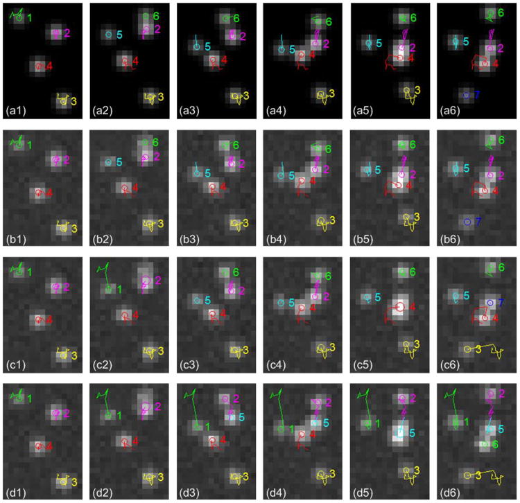
Trajectories obtained by the three methods (6 successive image frames are shown from left to right). Circles indicate center positions, and colored lines represent trajectories up to the current frame. (a1)–(a6) The ground truth trajectories on the images without noise. (b1)–(b6) Result from the proposed method 2M-E-MHT. (c1)–(c6) Result from the method 2M-s-MHT-b: trajectory 1 and 3 contain wrong links, and trajectory 2, 5, 6 and 7 are incomplete. (d1)–(d6) Result from the method 1M-s-MHT-a: trajectory 1, 2, 3 and 5 contain wrong links, and trajectory 4 and 6 are incomplete.
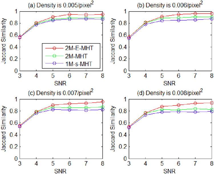
To evaluate the performance with a larger sliding time window, we set L = 5 and M = 1. We compare the proposed method 2M-E-MHT to the method 2M-MHT. The performance curves are shown in Fig. 10, and we re-plot those curves of the method 1M-s-MHT. The result shows that, by using the extended MHT framework, the proposed method does better than the method 2M-MHT when SNR is greater than 4.
Fig. 10.
Jaccard similarity scores of the three methods in all the scenarios.
To study the effect of the sliding time window in the proposed method, we vary the parameter L while keeping M = 1. The performance curves are shown in Fig. 11. The result shows that a longer window does not bring any significant benefit mostly because of the stochastic nature of the particle motion. Therefore, we use L = 2 and M = 1 as the default setting to process real data.
Fig. 11.
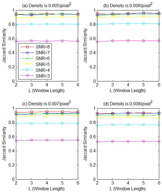
Jaccard similarity scores of the proposed method with different parameter L (window length).
B. Evaluation on Real Data
The goal is to study the effect of the molecular compound, methyl-β-cyclodextrin (MbCD) in clathrin mediated endocytosis. The plasma membrane is highly enriched in cholesterol. Plasma membrane cholesterol regulates biological processes occurring in this membrane, including endocytic events like clathrin mediated endocytosis. Indeed, clathrin mediated endocytosis was shown to be inhibited upon cholesterol extraction by methyl-β-cyclodextrin (MbCD) treatment [57], [58]. While CCPs are present after MbCD addition, as detected both by immunofluorescence for coat proteins on fixed cells and by electron microscopy, they are arrested at a shallow stage, suggesting a defect in maturation [57], which indicates that particle lifetimes should be longer after MbCD addition.
We have obtained TIRF movies of clathrin mediated endocytosis before and after MbCD addition. Wild type mouse fibroblasts were transiently transfected with GFP-tagged μ2 subunit of the clathrin adaptor protein 2 complex [59] by electroporation to visualize endocytic clathrin coats, and immediately plated at subconfluent densities onto fibronectin-coated 35mm glass bottom culture dishes (MatTek, Ashland, MA, USA). They were ready to be imaged after 24 hours. In each dish, a cell was randomly chosen as a sample of the group and then imaged. Images were acquired using a Nikon TiE inverted microscope equipped with 100 × oil objective lens (NA = 1.49). Excitation light was provided by 488nm diode-pumped solid-state lasers, coupled to the TIRF illuminator through an optical fiber. The output from the lasers was controlled by an acousto-optic tunable filter, and fluorescence signaling was acquired with an EM-CCD camera (DU-887; Andor). Acquisition was controlled by Andor iQ software. Images were sampled at 0.25 Hz with exposure times in the range of 100- to 500-ms. Cells were imaged at 37 °C for 10 minutes before the addition of MbCD to a final concentration of 10mM, and imaged for another 10 minutes.
We test the method on eight image datasets obtained by imaging four cells in four culture dishes before and after MbCD addition. Each dataset consists of about 150 image frames, and the size of an image is 512 × 512 pixels (1 pixel = 160nm), and the TIRF resolution in the xy-plane is about 200nm. After tracking, trajectories that start from the first image frame or end at the last image frame are considered to be incomplete, and discarded.
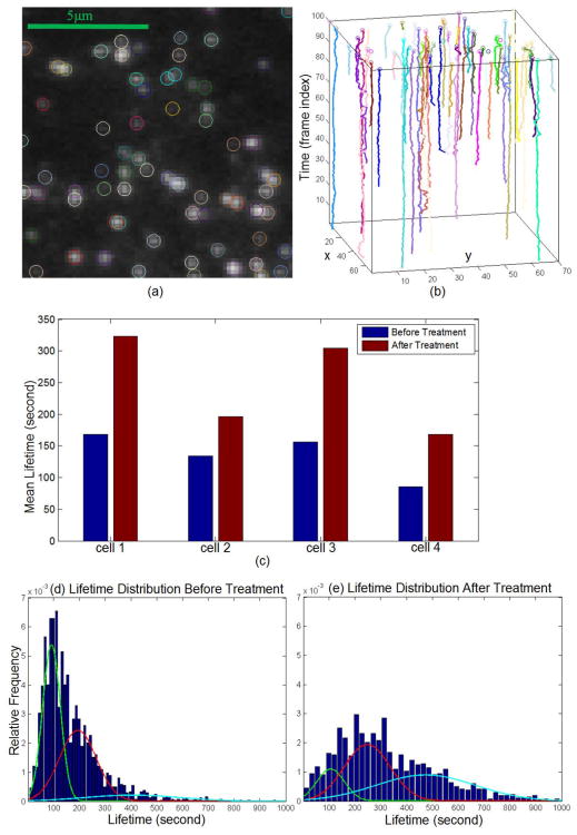
Examples of the detected particles and the recovered trajectories in an image region are shown in Fig. 12(a) and (b), respectively. As shown in Fig. 12(c), the mean lifetimes of the particles are significantly longer upon MbCD treatment (t-test: p-value < 0.001 in all the cases) which implies that MbCD significantly affected CME by prolonging particle lifetimes. On average, lifetime is increased by 82% after the treatment. To perform a subpopulation analysis as explained in [60], we plot the lifetime histograms before and after MbCD addition, and by using expectation-maximization algorithms, Gaussian mixture distribution functions are fitted to the histograms. As shown in Fig. 12(d) and (e), before the treatment, three particle subpopulations are identified with the average lifetimes of 93, 199 and 406 seconds, and after the treatment, three corresponding subpopulations are identified with the average lifetimes of 106, 248 and 474 seconds. The percentages of the three subpopulations changed from {48%, 42%, 10%} to {15%, 43%, 42%} after MbCD addition. The result suggests that different subpopulations may react differently upon the treatment which is a biological hypothesis [60].
Fig. 12.
(a) Detected particles in an image region, and colors are randomly assigned. (b) Trajectories over time, and colors are randomly assigned. (c) Mean lifetimes before and after MbCD treatment. (d) Lifetime distributions from cell #1 before MbCD treatment. (e) Lifetime distributions from cell #1 after MbCD treatment.
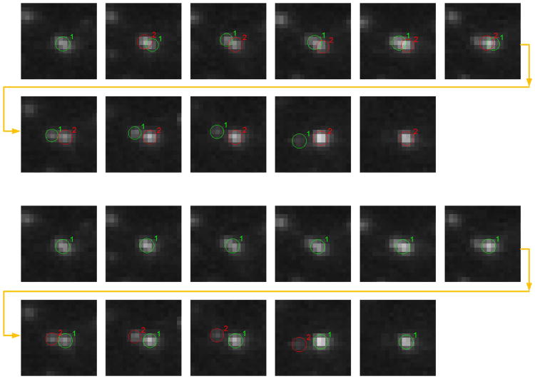
Although detailed biological analysis based on the tracking results is out of the scope of this paper, here we would like to present another type of biological analysis which is related to a kind of biological event that is not fully understood yet. It is known that during the CME process, some particles are generated almost at the same location, and such locations are called hotspots [61] in the literature. If two or more particles are created almost at the same location and coexist for a while, then their trajectories appear to be entangled on the image plane. As a result, the individual lifetimes of the particles can not be measured reliably. This uncertainty about individual lifetimes is caused by the inherent uncertainty of the data, and can not be solved by any algorithm currently, because biologists are still unable to label individual particles with different types of fluorophores. To perform lifetime analysis, the particles entangled at hotspots should be separated from the other particles. If a particle is created near another existing particle (set to be 3 pixels), and their trajectories are entangled over a few frames (set to be 2 frames), then the two particles are identified as being entangled at a hotspot. The lifetime of a hotspot can be defined to be the duration of a set of particles entangled at the same location, i.e., the duration from the time the first particle appears to the time the last particle disappears. Then we can analyze the lifetimes of hotspots in cells.
Our proposed method can automatically identify particles entangled at hotspots due to the advantage of the proposed E-MHT framework. However, since particle detection in MHT-based tracking methods is usually designed to be a completely independent module, these methods are unable to automatically identify such events. The mean lifetimes of hotspots in the cells before and after MbCD treatment are shown in Fig. 13. An example of a pair of particles entangled at a hotspot is shown in Fig. 14.
Fig. 13.
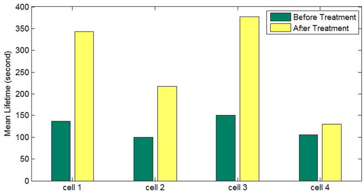
Mean lifetimes of hotspots in the cells before and after MbCD treatment, which are obtained by using our proposed method. The MHT-based methods with independent detection modules can not support such automatic analysis.
Fig. 14.
An example of a hotspot. The top sequence shows the result from our proposed method. The bottom sequence shows the result from the method 2M-MHT, and the results from the three representative MHT-based methods evaluated in section IV-A, are almost the same. The individual trajectories of the particles are unreliable due to the uncertainty of the data. Our proposed method can identify the hotspot where the two particles appear to be entangled. The MHT-based methods just find two independent particles/trajectories, and therefore can not identify them as being entangled at the hotspot.
V. Conclusion
We have proposed a particle tracking method for clathrin mediated endocytosis analysis. The classical MHT framework is extended by considering multiple observation candidates and more types of trajectory candidates, and the related optimization problem is solved by using integer programming. For CCP tracking, properties of the particles are considered in the models, and special strategies are designed for multiple candidate generation. The accuracy and robustness of the proposed method has been demonstrated by using synthetic datasets with different SNRs and particle densities. The method has been applied to analyze the real image data from the experiments to study the effect of the molecular compound, methyl-β-cyclodextrin (MbCD) in clathrin mediated exocytosis. The method can be extended for other applications by using appropriate models and detectors as suggested in [44]. We expect the method to be a good assistant for the biologists to investigate the mechanisms of clathrin mediated endocytosis and some other biological processes.
Acknowledgments
The authors thank Springer for letting them reuse some results/figures in the paper [44] published in Springer LNCS, which correspond to Fig. 1, Fig. 2(a)–(c), and Fig. 12(a) and (d) in this paper.
This work was supported in part by the Keck Foundation and in part by the NIH under Grants R37NS036251 and P30-DK45735. The associate editor coordinating the review of this manuscript and approving it for publication was Prof. Sina Farsiu.
Biographies

Liang Liang received the B.S. degree from Tsinghua University, China, in 2002, and the Ph.D. degree from Yale University, New Haven, CT, USA, in 2013.
His research interests include biomedical image analysis and computer vision. He focused on biological image analysis, including image reconstruction, object detection, and tracking.

Hongying Shen received the B.S. degree from Nanjing University, China, in 2006, and the Ph.D. degree from Yale University, New Haven, CT, USA, in 2013.
Her research interests include endocytic membrane trafficking and lipid metabolism. She focused on the mechanism how proteins and lipids components that regulates dynamics of endocytic process.

Pietro De Camilli is the Eugene Higgins Professor of cell biology and a Professor of neurobiology with Yale University, New Haven, CT, USA. He received the M.D. degree from the University of Milano in 1972 and the Postgraduate degree in medical endocrinology from the University of Pavia, Italy. He became an Investigator with the Howard Hughes Medical Institute in 1992. From 1997 to 2000, he served as a Chair of the Department of Cell Biology; and since 2005, he has been a Founding Director of the Yale Program in cellular neuroscience, neurodegeneration, and repair.
He is interested in the cell biology of neuronal synapses. His studies on synaptic vesicle dynamics have contributed to the general fields of exocytosis and endocytosis. His research has provided insight into mechanisms of membrane fission and has revealed ways through which membrane-associated proteins can generate, sense, and stabilize lipid bilayer curvature. His discovery and characterization of the role of phosphoinositide metabolism in the control of endocytosis have broad implications in the fields of phospholipid signaling and of membrane traffic. His studies of synapses have also contributed to the elucidation of pathogenetic mechanisms of human diseases.

James S. Duncan is the Ebenezer K. Hunt Professor of biomedical engineering and a Professor of diagnostic radiology and electrical engineering with Yale University, New Haven, CT, USA. He received the Ph.D. in electrical engineering from the University of Southern California, Los Angeles, in 1982.
His research and teaching efforts have been in the areas of computer vision, image processing and medical imaging, with an emphasis in biomedical image analysis. Currently, he is the Director of Undergraduate Studies and the Associate Chair of biomedical engineering and the Vice-Chair for Bioimaging Sciences research in Diagnostic Radiology. His specific research interests include the segmentation of deformable structure from 3D image data, the tracking of nonrigid motion/deformation from spatiotemporal images, and development of strategies for image-guided intervention/surgery. He has published over 220 peer-reviewed articles and has been the principal investigator on a number of peer-reviewed grants from the National Institutes of Health and the National Science Foundation. From 1973 to 1983, he was a member of the technical staff and Section Head at Hughes Aircraft Company, Electro-Optical and Data Systems Group, El Segundo, CA, USA, and joined the Yale Faculty in 1983. He is a member of Eta Kappa Nu and Sigma Xi, is a fellow of the American Institute for Medical and Biological Engineering and The MICCAI Society. He received the MICCAI 2008 Significant Researcher Award, given for his “pioneering research on Statistical and Deformable Model-Based Methods and their multiorgan-based applications.” He is on the editorial board of the Journal of Mathematical Imaging and Vision, is an Associate Editor for the IEEE Transactions on Medical Imaging and is one of the Founding Co-Editor-in-Chief of the journal Medical Image Analysis (Elsevier). He was a Fulbright Research Scholar at the Universities of Amsterdam and Utrecht, The Netherlands from 1993 to 1994. In 1997, he was Chair of the 15th international meeting on Information Processing in Medical Imaging and was the General Chair for the 2005 Meeting on Medical Image Computing and Computer-Assisted Intervention. From 1999 to 2003, he was a Charter Member of the National Institutes of Health Diagnostic Imaging Study Section, serving as its Chair from 2001 to 2003. In 2012, he was elected to the Council of Distinguished Investigators, Academy of Radiology Research.
Appendix A
The Proof
Here, we show Ê in Eq.(2) is the lower bound of the energy E in Eq.(1). For simplicity, the indicators are ignored here. We make a general assumption that is the true value of for each k. Firstly, is bounded because it can only reach its maximum when . Since the total number of targets/particles is finite, the second term in the right hand side of Eq.(3), i.e., has an upper bound ℳ. Secondly, it is obviously that log p(It|Dt) ≤ log p(It|Xt) with equality if Dt = HXt. Then:
Contributor Information
Liang Liang, Email: liang.liang@yale.edu, Department of Electrical Engineering, Yale University, New Haven, CT 06511 USA.
Hongying Shen, Email: hongying.shen@yale.edu, Department of Cell Biology, Yale University, New Haven, CT 06511 USA.
Pietro De Camilli, Email: pietro.decamilli@yale.edu, Department of Cell Biology, Yale University, New Haven, CT 06511 USA.
James S. Duncan, Email: james.duncan@yale.edu, Department of Electrical Engineering, Biomedical Engineering and Diagnostic Radiology, Yale University, New Haven, CT 06511 USA.
References
- 1.Mattheyses AL, Simon SM, Rappoport JZ. Imaging with total internal reflection fluorescence microscopy for the cell biologist. J Cell Sci. 2010 Nov;123:3621–3628. doi: 10.1242/jcs.056218. [DOI] [PMC free article] [PubMed] [Google Scholar]
- 2.Slepnev VI, Camilli PD. Accessory factors in clathrin-dependent synaptic vesicle endocytosis. Nature Rev Neurosci. 2000;1(3):161–172. doi: 10.1038/35044540. [DOI] [PubMed] [Google Scholar]
- 3.Kirchhausen T. Imaging endocytic clathrin structures in living cells. Trends Cell Biolo. 2009;20(1):596–605. doi: 10.1016/j.tcb.2009.09.002. [DOI] [PMC free article] [PubMed] [Google Scholar]
- 4.Shen H, et al. Constitutive activated Cdc42-associated kinase (Ack) phosphorylation at arrested endocytic clathrin-coated pits of cells that lack dynamin. Molecular Biol Cell. 2011;22(4):493–502. doi: 10.1091/mbc.E10-07-0637. [DOI] [PMC free article] [PubMed] [Google Scholar]
- 5.Saheki Y, Camilli PD. Synaptic vesicle endocytosis. Cold Spring Harbor Perspect Biol. 2012;4(9):1–30. doi: 10.1101/cshperspect.a005645. [DOI] [PMC free article] [PubMed] [Google Scholar]
- 6.Milosevic I, et al. Recruitment of endophilin to clathrin-coated pit necks is required for efficient vesicle uncoating after fission. Neuron. 2011;72(4):587–601. doi: 10.1016/j.neuron.2011.08.029. [DOI] [PMC free article] [PubMed] [Google Scholar]
- 7.Harold D, et al. Genome-wide association study identifies variants at CLU and PICALM associated with Alzheimer's disease, and shows evidence for additional susceptibility genes. Nature Genet. 2009;41(10):1088–1093. doi: 10.1038/ng.440. [DOI] [PMC free article] [PubMed] [Google Scholar]
- 8.Züchner S, et al. Mutations in the pleckstrin homology domain of dynamin 2 cause dominant intermediate charcot-marie-tooth disease. Nature Genet. 2005;37(3):289–294. doi: 10.1038/ng1514. [DOI] [PubMed] [Google Scholar]
- 9.Sorkin A, von Zastrow M. Endocytosis and signalling: Intertwining molecular networks. Nature Rev Molecular Cell Biol. 2009;10(9):609–622. doi: 10.1038/nrm2748. [DOI] [PMC free article] [PubMed] [Google Scholar]
- 10.Leto D, Saltiel AR. Regulation of glucose transport by insulin: Traffic control of GLUT4. Nature Rev Molecular Cell Biol. 2012;13(6):383–396. doi: 10.1038/nrm3351. [DOI] [PubMed] [Google Scholar]
- 11.Brandenburg B, Zhuang X. Virus trafficking—Learning from single-virus tracking. Nature Rev Microbiol. 2007;5(3):197–208. doi: 10.1038/nrmicro1615. [DOI] [PMC free article] [PubMed] [Google Scholar]
- 12.Smal I, Loog M, Niessen WJ, Meijering EHW. Quantitative comparison of spot detection methods in fluorescence microscopy. IEEE Trans Med Imag. 2010 Feb;29(2):282–301. doi: 10.1109/TMI.2009.2025127. [DOI] [PubMed] [Google Scholar]
- 13.Genovesio A, Liedl T, Emiliani V, Parak WJ, Coppey-Moisan M, Olivo-Marin JC. Multiple particle tracking in 3-D+t microscopy: Method and application to the tracking of endocytosed quantum dots. IEEE Trans Image Process. 2006 May;15(5):1062–1070. doi: 10.1109/tip.2006.872323. [DOI] [PubMed] [Google Scholar]
- 14.Qiu M, Lee HC, Yang G. Nanometer resolution tracking and modeling of bidirectional axonal cargo transport. Proc IEEE ISBI. 2012 Jun;:992–995. [Google Scholar]
- 15.Sage D, Neumann FR, Hediger F, Gasser SM, Unser M. Automatic tracking of individual fluorescence particles: Application to the study of chromosome dynamics. IEEE Trans Image Process. 2005 Sep;14(9):1372–1383. doi: 10.1109/tip.2005.852787. [DOI] [PubMed] [Google Scholar]
- 16.Godinez W, Lampe M, Wörz S, Müller B, Eils R, Rohr K. Deterministic and probabilistic approaches for tracking virus particles in time-lapse fluorescence microscopy image sequences. Med Image Anal. 2009;13(2):325–342. doi: 10.1016/j.media.2008.12.004. [DOI] [PubMed] [Google Scholar]
- 17.Jaiswal A, Godinez WJ, Eils R, Lehmann MJ, Rohr K. Tracking virus particles in fluorescence microscopy images using two-step multi-frame association. Proc 9th IEEE Int Symp Biomed Imaging. 2012 May;:664–667. doi: 10.1109/TIP.2015.2458174. [DOI] [PubMed] [Google Scholar]
- 18.Smal I, Draegestein K, Galjart N, Niessen WJ, Meijering EHW. Particle filtering for multiple object tracking in dynamic fluorescence microscopy images: Application to microtubule growth analysis. IEEE Trans Med Imaging. 2008 Jun;27(6):789–804. doi: 10.1109/TMI.2008.916964. [DOI] [PubMed] [Google Scholar]
- 19.Jaqaman K, et al. Robust single-particle tracking in live-cell time-lapse sequences. Nature Methods. 2008;5(8):695–702. doi: 10.1038/nmeth.1237. [DOI] [PMC free article] [PubMed] [Google Scholar]
- 20.Carter BC, Shubeita GT, Gross SP. Tracking single-particles: A user-friendly quantitative evaluation. Phys Biol. 2005;2(1):60–72. doi: 10.1088/1478-3967/2/1/008. [DOI] [PubMed] [Google Scholar]
- 21.Cheezum MK, Walker WF, Guilford WH. Quantitative comparison of algorithms for tracking single fluorescent particles. Biophys J. 2001;81(4):2378–2388. doi: 10.1016/S0006-3495(01)75884-5. [DOI] [PMC free article] [PubMed] [Google Scholar]
- 22.Kalaidzidis Y. Intracellular objects tracking. Eur J Cell Biol. 2007;86(9):569–578. doi: 10.1016/j.ejcb.2007.05.005. [DOI] [PubMed] [Google Scholar]
- 23.Feng L, Xu Y, Yang Y, Zheng X. Multiple dense particle tracking in fluorescence microscopy images based on multidimensional assignment. J Structural Biol. 2011;173(2):219–228. doi: 10.1016/j.jsb.2010.11.001. [DOI] [PubMed] [Google Scholar]
- 24.Acton ST, Ray N. Biomedical Image Analysis: Tracking. San Mateo, CA, USA: Morgan & Claypool; 2005. [Google Scholar]
- 25.Arulampalam MS, Maskell S, Gordon N, Clapp T. A tutorial on particle filters for online. nonlinear/non-Gaussian Bayesian tracking. IEEE Trans Signal Process. 2002 Feb;50(2):174–188. [Google Scholar]
- 26.Wen Q, Gao J, Luby-Phelps K. Multiple interacting subcellular structure tracking by sequential Monte Carlo method. Proc IEEE Int Conf Bioinformat Biomed. 2007 Nov;:437–442. doi: 10.1504/ijdmb.2009.026704. [DOI] [PubMed] [Google Scholar]
- 27.Greß O, Posch S. Trajectory retrieval from Monte Carlo data association samples for tracking in fluorescence microscopy images. Proc 9th IEEE Int Symp Biomed Imaging. 2012 May;:374–377. [Google Scholar]
- 28.Hue C, Cadre JPL, Pérez P. Sequential Monte Carlo methods for multiple target tracking and data fusion. IEEE Trans Signal Process. 2002 Feb;50(2):309–325. [Google Scholar]
- 29.Basden A, Haniff C, Mackay C. Photon counting strategies with low light level CCDs. Monthly Notices R Astronomical Soc. 2003;345(3):985–991. [Google Scholar]
- 30.Robbins MS, Hadwen BJ. The noise performance of electron multiplying charge-coupled devices. IEEE Trans Electron Devices. 2003 May;50(5):1227–1232. [Google Scholar]
- 31.Reid DB. An algorithm for tracking multiple targets. IEEE Trans Autom Control. 1979 Dec;24(6):843–854. [Google Scholar]
- 32.Chenouard N, Bloch I, Olivo-Marin JC. Multiple hypothesis tracking in microscopy images. Proc IEEE Int Symp Biomed Imaging, From Nano Macro. 2009 Jul;:1346–1349. [Google Scholar]
- 33.Yang G, Matov A, Danuser G. Reliable tracking of large-scale dense particle motion for fluorescent live cell imaging. Proc IEEE Comput Soc Conf Comput Vis Pattern Recognit Workshops. 2005 Jun;:130–138. [Google Scholar]
- 34.Poore AB. Some assignment problems arising from multiple target tracking. Math Comput Model. 2006;43(9–10):1074–1091. [Google Scholar]
- 35.Shafique K, Shah M. A noniterative greedy algorithm for multi-frame point correspondence. IEEE Trans Pattern Anal Mach Intell. 2005 Jan;27(1):51–65. doi: 10.1109/TPAMI.2005.1. [DOI] [PubMed] [Google Scholar]
- 36.Al-Kofahi O, Radke RJ, Goderie SK, Shen Q, Temple S, Roysam B. Automated cell lineage construction: A rapid method to analyze clonal development established with murine neural progenitor cells. Cell Cycle. 2006;5(3):327–335. doi: 10.4161/cc.5.3.2426. [DOI] [PubMed] [Google Scholar]
- 37.Padfield D, Rittscher J, Roysamb B. Coupled minimum-cost flow cell tracking for high-throughput quantitative analysis. Medical Image Anal. 2011;15(4):650–668. doi: 10.1016/j.media.2010.07.006. [DOI] [PubMed] [Google Scholar]
- 38.Thomann D, Rines DR, Sorger PK, Danuser G. Automatic fluorescent tag detection in 3D with super-resolution: Application to the analysis of chromosome movement. J Microscopy. 2002;208(1):49–64. doi: 10.1046/j.1365-2818.2002.01066.x. [DOI] [PubMed] [Google Scholar]
- 39.Xu R, W D., II Survey of clustering algorithms. IEEE Trans Neural Netw. 2005 May;16(3):645–678. doi: 10.1109/TNN.2005.845141. [DOI] [PubMed] [Google Scholar]
- 40.Figueiredo MA, Jain AK. Unsupervised learning of finite mixture models. IEEE Trans Pattern Anal Mach Intell. 2002 Mar;24(3):1–16. [Google Scholar]
- 41.Genovesio A, Olivo-Marin JC. Split and merge data association filter for dense multi-target tracking. Proc 17th Int Conf Pattern Recognit. 2004 Aug;:677–680. [Google Scholar]
- 42.Liang L, Shen H, Camilli PD, Duncan JS. Tracking clathrin coated pits with a multiple hypothesis based method. Med Image Comput Comput Assist Intervent. 2010 Jan;13:315–322. doi: 10.1007/978-3-642-15745-5_39. [DOI] [PMC free article] [PubMed] [Google Scholar]
- 43.Liang L, Xu Y, Shen H, Camilli PD, Toomre D, Duncan JS. Automatic detection of subcellular particles in fluorescence microscopy via feature clustering and Bayesian analysis. Proc IEEE Workshop Math Methods Biomed Image Anal. 2012 Jan;:161–166. [Google Scholar]
- 44.Liang L, Shen H, Rompolas P, Greco V, Camilli PD, Duncan JS. A multiple hypothesis based method for particle tracking and its extension for cell segmentation. Proc 23rd Int Conf Inf Process Med Imaging. 2013:98–109. doi: 10.1007/978-3-642-38868-2_9. [DOI] [PMC free article] [PubMed] [Google Scholar]
- 45.Li XR, Jilkov VP. Survey of maneuvering target tracking. Part I. Dynamic models. IEEE Trans Aerosp Electron Syst. 2003 Oct;39(4):1333–1364. [Google Scholar]
- 46.Li XR, Jilkov VP. Survey of maneuvering target tracking. Part V. Multiple-model methods. IEEE Trans Aerosp Electron Syst. 2005 Jan;41(4):1255–1321. [Google Scholar]
- 47.Smith K, Carleton A, Lepetit V. General constraints for batch multiple-target tracking applied to large-scale videomicroscopy. Proc IEEE Conf Comput Vis Pattern Recognit. 2008 Jun;:1–8. [Google Scholar]
- 48.Blom HA, Bar-Shalom Y. The interacting multiple model algorithm for systems with Markovian switching coefficients. IEEE Trans Autom Control. 1988 Aug;33(8):780–783. [Google Scholar]
- 49.Li K, Chen M, Kanade T, Miller E, Weiss L, Campbell P. Cell population tracking and lineage construction with spatiotemporal context. Med Image Anal. 2008 Oct;12(5):546–566. doi: 10.1016/j.media.2008.06.001. [DOI] [PMC free article] [PubMed] [Google Scholar]
- 50.Zhang B, Zerubia J, Olivo-Marin JC. Gaussian approximations of fluorescence microscope point-spread function models. Appl Opt. 2007;46(10):1819–1829. doi: 10.1364/ao.46.001819. [DOI] [PubMed] [Google Scholar]
- 51.Kong TY, Rosenfeld A. Topological Algorithms for Digital Image Processing. New York, NY, USA: Elsevier; 1996. [Google Scholar]
- 52.Stock K, Sailer R, Strauss WSL, Lyttek M, Steiner R, Schneckenburger H. Variable-angle total internal reflection fluorescence microscopy (VA-TIRFM): Realization and application of a compact illumination device. J Microscopy. 2003;211(1):19–29. doi: 10.1046/j.1365-2818.2003.01200.x. [DOI] [PubMed] [Google Scholar]
- 53.Rohrbach A. Observing secretory granules with a multiangle evanescent wave microscope. Biophys J. 2000;78(5):2641–2654. doi: 10.1016/S0006-3495(00)76808-1. [DOI] [PMC free article] [PubMed] [Google Scholar]
- 54.Yang Q, Karpikov A, Toomre D, Duncan JS. 3-D reconstruction of microtubules from multi-angle total internal reflection fluorescence microscopy using Bayesian framework. IEEE Trans Image Process. 2011 Aug;20(8):2248–2259. doi: 10.1109/TIP.2011.2114359. [DOI] [PubMed] [Google Scholar]
- 55.Liang L, Shen H, Xu Y, Camilli PD, Toomre D, Duncan JS. A Bayesian method for 3D estimation of subcellular particle features in multi-angle TIRF microscopy. Proc 9th IEEE Int Symp Biomed Imaging. 2012 May;:984–987. [Google Scholar]
- 56.Kasturi R, et al. Framework for performance evaluation of face, text, and vehicle detection and tracking in video: Data, metrics, and protocol. IEEE Trans Pattern Anal Mach Intell. 2009 Feb;31(2):319–336. doi: 10.1109/TPAMI.2008.57. [DOI] [PubMed] [Google Scholar]
- 57.Rodal S, Skretting G, Garred O, Vilhardt F, van Deurs B, Sandvig K. Extraction of cholesterol with methyl-beta-cyclodextrin perturbs formation of clathrin-coated endocytic vesicles. MolBiol Cell. 1999;10(4):961–974. doi: 10.1091/mbc.10.4.961. [DOI] [PMC free article] [PubMed] [Google Scholar]
- 58.Subtil A, Gaidarov I, Kobylarz K, Lampson M, Keen J, McGraw T. Acute cholesterol depletion inhibits clathrin-coated pit budding. Proc Nat Acad Sci United States Amer. 1999;96(12):6775–6780. doi: 10.1073/pnas.96.12.6775. [DOI] [PMC free article] [PubMed] [Google Scholar]
- 59.Zoncu R, et al. Loss of endocytic clathrin-coated pits upon acute depletion of phosphatidylinositol 4,5-bisphosphate. Proc Nat Acad Sci United States Amer. 2007;104(10):3793–3798. doi: 10.1073/pnas.0611733104. [DOI] [PMC free article] [PubMed] [Google Scholar]
- 60.Loerke D, et al. Cargo and dynamin regulate clathrin-coated pit maturation. PLoS Biol. 2009;7(3):e1000057. doi: 10.1371/journal.pbio.1000057. [DOI] [PMC free article] [PubMed] [Google Scholar]
- 61.Saffarian S, Cocucci E, Kirchhausen T. Distinct dynamics of endocytic clathrin-coated pits and coated plaques. PLoS Biol. 2009;7(9):1–18. doi: 10.1371/journal.pbio.1000191. [DOI] [PMC free article] [PubMed] [Google Scholar]


