Principal Component Analysis as a Tool for Library Design: A Case Study Investigating Natural Products, Brand-Name Drugs, Natural Product-Like Libraries, and Drug-Like Libraries

Abstract

Principal component analysis (PCA) is a useful tool in the design and planning of chemical libraries. PCA can be used to reveal differences in structural and physicochemical parameters between various classes of compounds by displaying them in a convenient graphical format. Herein, we demonstrate the use of PCA to gain insight into structural features that differentiate natural products, synthetic drugs, natural product-like libraries, and drug-like libraries, and show how the results can be used to guide library design.

1 Introduction

Principal component analysis (PCA) is a mathematical method for dimensionality reduction that allows for multidimensional datasets to be visualized using two- or three-dimensional plots with minimal loss of information [1, 2]. When applied in the context of diversity-oriented synthesis, PCA is primarily used to visualize similarities and differences within collections of compounds based on structural and physicochemical parameters, and can be leveraged in library design [3]. Molecular weight, stereocenters, rotatable bonds, hydrophobicity, and aqueous solubility are a few examples of parameters commonly included in such analyses. Herein, we selected 20 structural and physicochemical parameters for analysis based on previously identified correlations of these parameters with oral bioavailability, cell permeability, solubility, and binding selectivity, as well as their ability to distinguish synthetic drugs from natural products (vide infra). Each compound in our analysis is represented as a 20-dimensional vector defined by the structural and physicochemical parameters. PCA rotates these vectors onto a new set of orthogonal axes called principal components, in which the variance retained from the original data is maximized on each successive principal component. As such, the three-dimensional plot we show in this example retains 75 % of the variance from the full 20-dimensional dataset.

PCA can also be used to guide the design of chemical libraries. This is important in drug discovery because current drugs are limited in both structure and function. For example, current small-molecule drugs address only about 1 % of the protein targets encoded in the human genome [4], and half of those target only four protein classes: rhodopsin-like G-protein receptors, nuclear receptors, and voltage- and ligand-gated ion channels. In contrast, natural products are known to target a broader range of protein classes and have led to the majority of antibacterials (65 %) and anticancer drugs (75 %) [5]. Therefore, novel libraries of compounds that share the structural features of natural products are attractive for the discovery of lead compounds to evaluate new therapeutic targets.

Along these lines, many macrocycle and medium-ring-containing natural products have compelling biological activities. This key cyclic framework presents functional groups to biological targets in appropriate pharmacophoric conformations [6–8]. Compared to their corresponding linear congeners, macrocycles can provide increased binding affinity [9], improved bioavailability [10], and, in some cases, enhanced cell permeability [11], which are desirable pharmacological properties in the development of new drugs.

However, despite these attractive features of macrocycles and medium rings, they remain severely underexploited in current drug and probe discovery efforts [12, 13], due to challenges associated with their synthesis. To address the underrepresentation of these compounds, we have sought to circumvent the inherent limitations of classical cyclization-based strategies for macrocycle and medium-ring synthesis by developing alternative ring-expansion approaches that are tolerant of a broad range of substitution patterns and functional groups. We recently developed two such methods (Fig. 1) [12, 13], both of which can be employed on gram scale, provide products bearing handles for further diversification, and are transferable to parallel synthesis platforms.

Fig. 1.

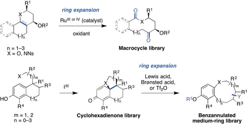
Recently developed routes to natural product-like macrocycle and medium-ring libraries using ring expansion strategies

Herein, we describe the use of PCA to assess how libraries of compounds produced using these synthetic routes compare to natural products and what structural and physicochemical parameters distinguish them from synthetic drugs and drug-like libraries. The information harnessed from PCA can also direct downstream modifications of a scaffold to obtain molecules that are more characteristic of a targeted class, such as natural products.

In this example, we show that compounds appearing in the proximity of the drug-like region of the PCA plot can be modified to have greater natural product-like properties by addressing several influential structural and physicochemical parameters. The relative contributions of structural and physicochemical parameters to each principal component (PC) axis are obtained from the loading data and loading plots produced from PCA. In the analysis presented herein, the number of oxygen atoms, hydrogen bond donors, and hydrogen bond acceptors are among the most influential parameters for PC1. Stereochemical density (the number of stereocenters normalized to molecular weight) and the fraction of sp³-hybridized carbons are large contributors to PC2. We further demonstrate that these structural and physicochemical parameters can be addressed by chemical modifications of our library members to increase their natural product-like character. Subsequent analysis of these modified compounds in PCA demonstrates their increased penetration into natural product-like regions of the plot. This work illustrates how insights gleaned from PCA can be used in the planning of chemical libraries to probe targeted areas of chemical space.

2 Materials

This analysis requires the use of several software packages that are either commonly available in chemistry labs or freely available for download. The following software and versions were used for this protocol:

1. Mac OS 10.5.8 or Windows 7 (procedure described for Mac OS with specific changes for Windows 7 users indicated).

2. CS ChemBioDraw Ultra 12.0.3 (CambridgeSoft).

3. Microsoft Office 2008.

4. Instant JChem 5.3.8 (ChemAxon, free Academic License available).

5. Virtual Computational Chemistry (VCC) Laboratory: http://www.vcclab.org/lab/alogps/start.html (requires a JAVA-enabled browser).

6. R 2.9.2 (open-source R Project for Statistical Computing, available from http://www.r-project.org).

3 Methods

3.1 Calculation of Physicochemical Parameters

1. Obtain SMILES codes for all of the compounds to be included in the PCA (see ^{Notes 1} and ²). SMILES codes for known compounds can be obtained from PubChem (http://pubchem.ncbi.nlm.nih.gov/) or other online resources. For new compounds, SMILES codes can be generated using ChemBioDraw (see ^{Note 3}).

2. Create a new MS Excel file containing one column for compound names (Column A) and one column for SMILES codes (Column B) (see ^{Note 4}). Do not include a header row. Group the compounds by compound class (such as Drugs, Natural Products). Save the MS Excel file as a Text (tab delimited) (.txt) file that will be used in Subheading 3.1, step 4. Delete the compound names column and save an additional .txt file that contains only SMILES codes, which will be used later will be used later for batch processing (Subheading 3.1, step 7).

3. Using Instant JChem, open a new project (File > New Project), and click on “Next” (see ^{Note 5}). Enter a project name and then click on “Finish”.

4. From Instant JChem, import the MS Excel file containing the compound names and SMILES codes by selecting File > Import File, and then click on “Next” (see ^{Note 6}). Click on the folder icon next to the “File to import” field, and then navigate to and select the .txt file containing compound names and SMILES codes. Under “File Format” choose “Delineated text files (*.csv, *.tab, *.txt)”, and then click on “Open”. After Instant JChem has finished scanning the file and indicated the number of fields found, click on “Next”. The “Field details” panel gives a summary of the fields to be imported from the text file. The structure, molecular weight, molecular formula, and compound names of each entry are displayed by default (see ^{Note 7}). The “Monitor import” window will give a summary of the imported data (see ^{Note 8}). Once fully processed, click on “Finish”.

5. Use Instant JChem to determine values for physicochemical properties by selecting Data > New Chemical Term Field. Use the “Expression” drop-down menu to choose preset chemical terms (see ^{Notes 9} and ¹⁰). Enter an appropriate Name for the column and then click on “Finish” (Fig. 2). For this example, we selected the following 16 terms (Instant JChem input syntax follows each description) (see ^{Notes 11} and ¹²):

   • Molecular weight (MW): mass()
   • N atom count (N): atomCount(“7”)
   • O atom count (O): atomCount(“8”)
   • H-bond donor count (HBD): donorCount()
   • H-bond acceptor (HBA): acceptorCount()
   • Rotatable bond count (RotB): rotatableBondCount()
   • Stereocenter count (nStereo): chiralCenterCount()
   • Topological polar surface area (tPSA): PSA()
   • Number of rings (Rings): ringCount()
   • Aromatic ring count (RngAr): aromaticRingCount()
   • Ring system count (RngSys): ringSystemCount()
   • Size of largest ring (RngLg): largestRingSize()
   • Fraction of sp³-hybridized carbons (Fsp3): count(filter(‘atno()==6 && connections()==4’))/atomCount(“6”)
   • n-Octanol/water partition coefficient at pH = 7.4 (LogD): logd(‘7.4’)
   • van der Waals surface area (VWSA): vanDerWaalsSurfaceArea()
   • Relative polar surface area (relPSA): PSA()/vanDerWaals SurfaceArea()

6. Export the table of physicochemical parameters calculated in Instant JChem to an MS Excel file (.xls) by selecting File > Export to File. In the “Specify details” window, click on the purple folder to the right of the “File” field. Name the file and define the file format as “Microsoft Office Excel Workbook (*xls)”. The following window gives the user an option to remove or rearrange columns in the exported file (see ^{Note 13}). The “Monitor progress” window summarizes the export process. When complete, click on “Finish”. Open the .xls file containing these physicochemical parameters in MS Excel; additional physicochemical parameters will be added later (Subheading 3.1, steps 8 and 9).

7. The following two physicochemical values are calculated using the VCC Lab Website (http://www.vcclab.org/lab/alogps/start.html) (see ^{Notes 12} and ¹⁴):

   • n-Octanol/water partition coefficient alt (ALOGPs)
     Tetko’s logS aqueous solubility (ALOGpS)

   To calculate ALOGPs and ALOGpS from the website’s window, choose “Upload file” and select “Smiles—SMILES file—default” from the drop-down menu and click on “Proceed with file uploading” (Fig. 3). Click on “Choose file” and select the .txt file consisting of SMILES codes only that was created in Subheading 3.1, step 2. Click on “Upload file” and a new pop-up window should be displayed that states “Your file “yourfile.txt” was uploaded successfully.” Close the pop-up window displaying this message and a new window will open that is entitled “results.txt”. Copy the text from this results window and paste it into a new MS Excel file.

8. In the MS Excel sheet/tab that contains the physicochemical parameters calculated by Instant JChem (Subheading 3.1, step 6), add two new columns labeled “ALOGPs” and “ALOGpS.” Copy the “logP” and “logS” data columns calculated by the VCC Lab website, and paste them into the “ALOGPs” and “ALOGpS” columns, respectively. Close the MS Excel file that contains only the VCC Lab data.

9. The remaining two physicochemical parameters are calculated in MS Excel (see ^{Note 12}):

   • nStereo ÷ MW, stereochemical density (nStMW)
   • Rings ÷ RingSys, ring complexity (RRSys)
   Create two new columns in the MS Excel file that contains the other physicochemical values. For the nStMW and RRSys columns, set the column’s formula according to its respective equation (Fig. 4):

   • nStMW = [column for nStereo]/[column for MW]
   • RRSys = IF([column for RingsSys] = 0,0,[column for Rings]/[column for RingSys]) (see ^{Note 15}).
   • All of the physicochemical parameters needed for this PCA are now in the MS Excel file.

Fig. 2.

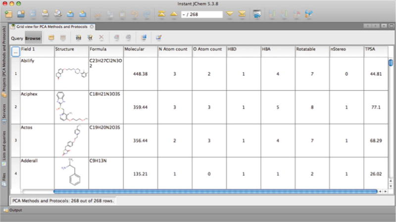
Instant JChem table showing selected chemical terms (physicochemical parameters) used for PCA

Fig. 3.

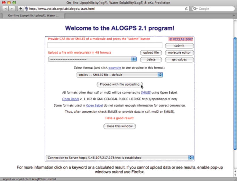
Uploading SMILES codes to calculate ALOGpS and ALOGPs at the VCC Lab Website

Fig. 4.

Final physicochemical parameters calculated in MS Excel, with the RRsys calculation in cell T2 and the referenced cells M2 and 02 highlighted as an example

3.2 Principal Component Analysis

1. In the MS Excel file containing the compound names and physicochemical parameters that was created in Subheading 3.1, verify that the compounds are grouped by compound class (such as Drugs, Natural Products), and insert a new row below each group. Each new row will represent the average compound for a given class. Accordingly, name each new row based on the category it will represent, for example “AVG Drug”. For these new rows, fill the cells associated with structural and physicochemical parameter values using the “AVERAGE” function to the left of the cell formula field and select the appropriate cells. Similarly, add two new rows below the last compound and calculate the mean (“AVERAGE”) of each physicochemical parameter for the entire dataset (all compounds), as well as the standard deviation of each parameter using the “STDEV” function. Name the MS Excel sheet/tab “Raw”.

2. Create a new sheet/tab within the same MS Excel file, naming it “Norm” to contain mean normalized values of the physicochemical parameters. Copy the compound names from the row header and physicochemical descriptors from the column header of the “Raw” sheet/tab and paste them into this “Norm” sheet/tab. Fill each standardized physicochemical parameter cell with the Normval value calculated using the equation

   Normval = ([val] – [column mean])/[column standard deviation]

   where “val” is the value from the corresponding cell in the “Raw” sheet/tab. The number format (Format > Cells…) should be set to four decimal places. Save the MS Excel file. Now, save only the “Norm” sheet/tab as “Data.txt” (Text-Tab Delimited) on the Desktop (Mac). Close the MS Excel file and discard the changes to the file format.

3. Launch the “R” open-source computing package and run the following PCA commands (at the command prompt “R>”) (see ^{Note 16}):

   • R > read.table(“~/Desktop/Data.txt”) – > a
   • R > prcomp(a) – > b
   • R > summary(b)

   This command gives a table showing the distribution of variance from the full dataset on each principal component (Fig. 5). PCA generates as many principal components as there are parameters, but importantly, the majority of variance is represented in the first few components (see refs. 1, 2 for further discussion on PCA and variance). In this example, the first three principal components (PC1–PC3) retain 75 % of the variance from the 20-dimensional dataset. As such, PC1–PC3 can be used to construct a set of two-dimensional plots that will allow the visualization of the data in a more intuitive manner while still retaining the majority of the information from the full dataset. We will therefore focus our remaining analysis on PC1–PC3.

4. To obtain loading information for each structural and physicochemical parameter, continue PCA with the following command in “R”:

   • R > b

   The resulting table can be copied into MS Excel for convenient access (see ^{Note 17}) (Fig. 6). The loading data will become useful for directing future library design and will be discussed in Subheading 3.3.

5. Obtain loading plots in “R” using the following command:

   • R > biplot(b, choices = c(1, 2), col = c(“gray”, “red”))

   The plot produced illustrates loading data of structural and physicochemical parameters for PC1 vs. PC2 (see ^{Notes 18} and ¹⁹) (Fig. 7). Save the loading plot and name it appropriately (see ^{Note 20}).

6. Generate loading plots of PC1 vs. PC3 and PC3 vs. PC2, using the following commands (and saving each loading plot):

   • R > biplot(b, choices = c(1, 3), col = c(“gray”, “red”))
   • R > biplot(b, choices = c(3, 2), col = c(“gray”, “red”))

   These loading plots give insight into the structural and physicochemical parameters that most distinguish a set of compounds by visually displaying each physicochemical parameter’s influence on where a compound will appear in the final PCA plots. This information is also valuable to the planning of future libraries and is discussed in Subheading 3.3.

7. In “R”, use the following commands to obtain the rotated PCA data (scores) and save the output as a text file (see ^{Note 21}):

   • R > b$x – > c
   • R > write.table(c, “~/Desktop/scores.txt”, sep = “\t”)

8. Open the MS Excel file that contains the “Raw” and “Norm” sheets/tabs (Subheading 3.2, step 2), and create a new sheet/tab within that MS Excel file, naming it “PCA”. To transfer the scores data obtained from “R” to MS Excel, first open the scores.txt file in a text editor. At the beginning of the document, add a column header such as “Compound” followed by a tab (Fig. 8). Next, copy all of the text in the file and paste it into the MS Excel sheet/tab named “PCA”. Change the number format (Format > Cells…) of the PCA cells to three decimal places.

9. In MS Excel, plot PC1 vs. PC2 from the “PCA” sheet/tab by selecting the columns and clicking on the “Chart Wizard” icon in the Standard Toolbar (View > Toolbars > Standard). Under “Standard Types” choose “Scatter XY” and click on “Next”. Enter series information (e.g., Drugs, Natural Products) under the “Series” tab and fill the X- and Y-values data fields with corresponding range for each series (for example PC1 data for X-values and PC2 data for Y-values). When done entering the series information, click on “Next”. Enter a title for the plot and labels for the axes and then click on “Next.” Select “As object in PCA” and click on “Finish” (see ^{Note 22}).

10. Follow a procedure similar to that described in Subheading 3.2, step 9, to generate plots for PC1 vs. PC3 and PC3 vs. PC2 using the data from the appropriate columns.

11. Copy the plots produced in MS Excel and use MS PowerPoint or graphical editing software to add colored ovals that encompass the majority of data points for a given class of compounds (Fig. 9).

Fig. 5.

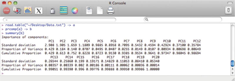
“R” output showing the variance retained in each successive principal component of the PCA

Fig. 6.

Coefficients of each parameter used for PC1–PC3, highlighting those of the greatest magnitude

Fig. 7.

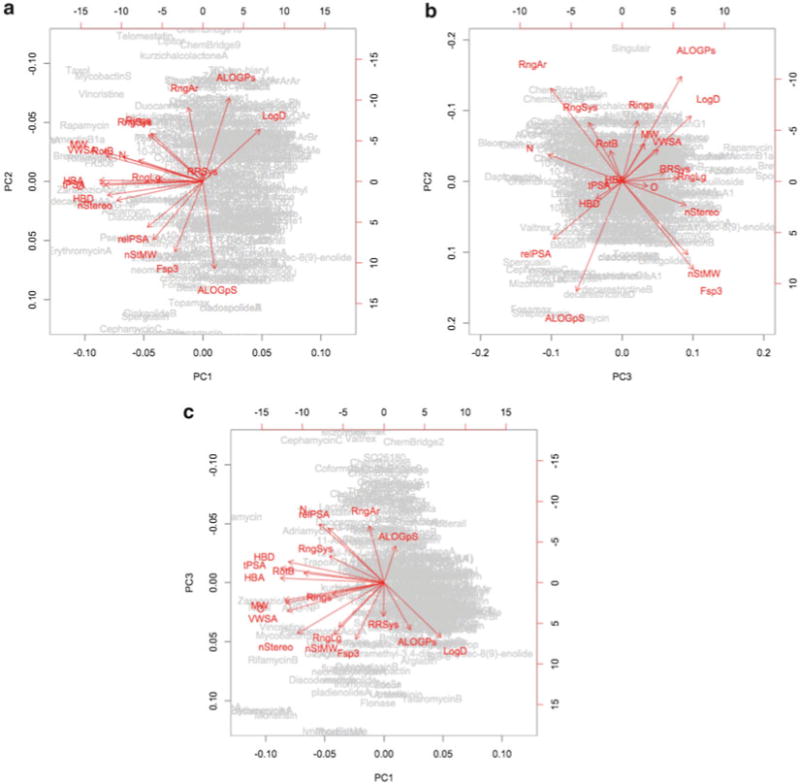
Loading plots from PCA: (a) PC1 vs. PC2, (b) PC2 vs. PC3, (c) PC1 vs. PC 3

Fig. 8.

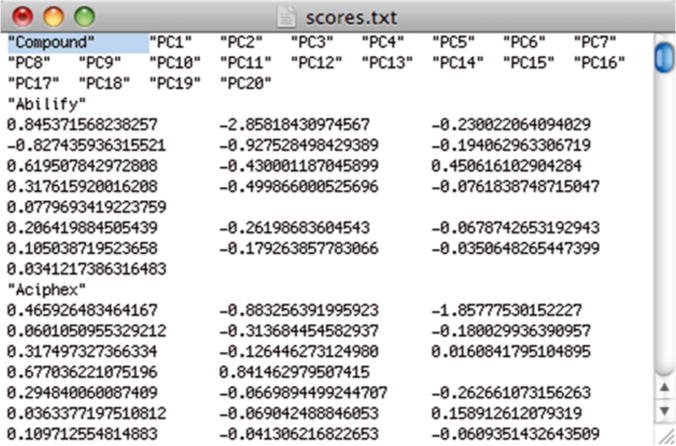
Modified PCA scores.txt file including a header for compound names

Fig. 9.

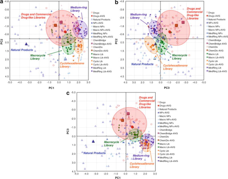
Completed PCA plots: (a) PC1 vs. PC2, (b) PC2 vs. PC3, (c) PC1 vs. PC 3

3.3 Using PCA to Guide Library Design

1. Examine the PCA plots together with the loading plots to identify structural and physicochemical parameters that determine where a particular compound or a collection of compounds appears on the PCA plot. For example, many natural products appear to the left (negative PC1) of the library members in the PC1 vs. PC2 plot (Fig. 9). The corresponding loading plot (Fig. 7) indicates that HBA, tPSA, and O are all major components of PC1. Recalling that each PC axis is a linear combination of structural and physicochemical parameters, Note that the coefficients for each parameter used for a given PC axis were also obtained in Subheading 3.2, step 4 (Fig. 6). This table provides more quantitative information regarding the parameters that have the greatest impact on the location of a compound with respect to each PC axis.

2. Consider the structural and physicochemical parameters that are the most important in differentiating a collection of compounds from the targeted region of chemical space. In this example, O, HBD, HBA, tPSA, nStereo, aqueous solubility, and Fsp³ are among the most influential in distinguishing our library compounds from natural products. The introduction of additional oxygen atoms and additional stereocenters to our library compounds would likely lead to more natural product-like compounds. A dihydroxylation of the olefins contained in our medium-ring library members would address all of the parameters mentioned above and should result in compounds that are shifted towards natural products in our PCA plots. Leveraging this information, we proceed with the dihydroxylation of multiple medium-ring compounds to produce a collection of PCA-directed derivatives of our initial medium-ring library.

3. Include the collection of modified compounds in a new analysis to evaluate the effectiveness of the PCA-directed modifications in targeting the desired region of the plot (Fig. 10). In this example, our diol products have structural and physicochemical parameters that are more consistent with natural products compared to their parent olefins, and as a result, the compounds are shifted towards natural products in all of the PCA plots. Reiterate this process as necessary to provide a library with the desired structural and physicochemical properties.

Fig. 10.

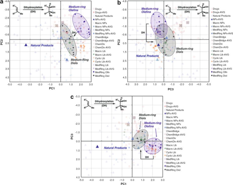
Completed PCA plots: (a) PC1 vs. PC2, (b) PC2 vs. PC3, (c) PC1 vs. PC 3. DH = dihydroxylation

References

- 1.Jolliffe IT. Principal component analysis. Springer; New York, NY: 2002. [Google Scholar]
- 2.Jackson JE. A user’s guide to principal components. Wiley; Hoboken, NJ: 2003. [Google Scholar]
- 3.Akella LB, DeCaprio D. Cheminformatics approaches to analyze diversity in compound screening libraries. Curr Opin Chem Biol. 2010;14:325–330. doi: 10.1016/j.cbpa.2010.03.017. [DOI] [PubMed] [Google Scholar]
- 4.Overington JP, Al-Lazikani B, Hopkins AL. How many drug targets are there? Nat Rev Drug Discov. 2006;5:993–996. doi: 10.1038/nrd2199. [DOI] [PubMed] [Google Scholar]
- 5.Newman DJ, Cragg GM. Natural products as sources of new drugs over the 30 years from 1981 to 2010. J Nat Prod. 2012;75:311–335. doi: 10.1021/np200906s. [DOI] [PMC free article] [PubMed] [Google Scholar]
- 6.Sánchez-Pedregal VM, et al. The tubulin- bound conformation of discoder-molide derived by NMR studies in solution supports a common pharmacophore model for epothilone and discodermolide. Angew Chem Int Ed. 2006;45:7388–7394. doi: 10.1002/anie.200602793. [DOI] [PubMed] [Google Scholar]
- 7.Canales A, et al. The bound conformation of microtubule-stabilizing agents: NMR insights into the bioactive 3D structure of discodermolide and dictyostatin. Chem Eur J. 2008;14:7557–7569. doi: 10.1002/chem.200800039. [DOI] [PubMed] [Google Scholar]
- 8.Knust J, Hoffmann RW. Synthesis and conformational analysis of macrocyclic dilactones mimicking the pharmacophore of aplysiatoxin. Helv Chim Acta. 2003;86:1871–1893. [Google Scholar]
- 9.Khan AR, et al. Lowering the entropic barrier for binding conformationally flexible inhibitors to enzymes. Biochemistry. 1998;37:16839–16845. doi: 10.1021/bi9821364. [DOI] [PubMed] [Google Scholar]
- 10.Veber DF, et al. Molecular properties that influence the oral bioavailability of drug candidates. J Med Chem. 2002;45:2615–2623. doi: 10.1021/jm020017n. [DOI] [PubMed] [Google Scholar]
- 11.Rezai T, et al. Testing the conformational hypothesis of passive membrane permeability using synthetic cyclic peptide diastereomers. J Am Chem Soc. 2007;128:2510–2511. doi: 10.1021/ja0563455. [DOI] [PubMed] [Google Scholar]
- 12.Kopp F, et al. A diversity-oriented synthesis approach to macrocycles via oxidative ring expansion. Nat Chem Biol. 2012;8:358–365. doi: 10.1038/nchembio.911. [DOI] [PMC free article] [PubMed] [Google Scholar]
- 13.Bauer RA, Wenderski TA, Tan DS. Biomimetic diversity-oriented synthesis of benzannulated medium rings via ring expansion. Nat Chem Biol. 2013;9:21–29. doi: 10.1038/nchembio.1130. [DOI] [PMC free article] [PubMed] [Google Scholar]
- 14.Lipinski CA, et al. Experimental and computational approaches to estimate solubility and permeability in drug discovery and development settings. Adv Drug Deliv Rev. 1997;23:3–25. doi: 10.1016/s0169-409x(00)00129-0. [DOI] [PubMed] [Google Scholar]
- 15.Tetko IV, et al. Estimation of aqueous solubility of chemical compounds using E-state indices. J Chem Inf Comput Sci. 2001;41:1488–1493. doi: 10.1021/ci000392t. [DOI] [PubMed] [Google Scholar]
- 16.Feher M, Schmidt JM. Property distributions: differences between drugs, natural products, and molecules from combinatorial chemistry. J Chem Inf Comput Sci. 2003;43:218–227. doi: 10.1021/ci0200467. [DOI] [PubMed] [Google Scholar]
- 17.Lovering F, Bikker J, Humblet C. Escaping from flatland: increasing saturations as an approach to improving clinical success. J Med Chem. 2009;52:6752–6756. doi: 10.1021/jm901241e. [DOI] [PubMed] [Google Scholar]
- 18.Clemons PA, et al. Small molecules of different origins have distinct distributions of structural complexity that correlate with protein-binding profiles. Proc Natl Acad Sci U S A. 2010;107:18787–18792. doi: 10.1073/pnas.1012741107. [DOI] [PMC free article] [PubMed] [Google Scholar]
- 19.O’Shea R, Moser HM. Physicochemical properties of antibacterial compounds: implications for drug discovery. J Med Chem. 2008;51:2871–2878. doi: 10.1021/jm700967e. [DOI] [PubMed] [Google Scholar]
- 20.McGrath NA, Brichacek M, Njardarson JT. A graphical journey of innovative organic architectures that have improved our lives. J Chem Educ. 2010;87:1348–1349. Also see also: Njardarson Group—Top top-selling drugs Pharmaceuticals poster; http://cbc.arizona.edu/njardarson/group/top-pharmaceuticals-poster. [Google Scholar]