Delay Differential Analysis of Time Series

Abstract

Nonlinear dynamical system analysis based on embedding theory has been used for modeling and prediction, but it also has applications to signal detection and classification of time series. An embedding creates a multidimensional geometrical object from a single time series. Traditionally either delay or derivative embeddings have been used. The delay embedding is composed of delayed versions of the signal, and the derivative embedding is composed of successive derivatives of the signal. The delay embedding has been extended to nonuniform embeddings to take multiple timescales into account. Both embeddings provide information on the underlying dynamical system without having direct access to all the system variables. Delay differential analysis is based on functional embeddings, a combination of the derivative embedding with nonuniform delay embeddings. Small delay differential equation (DDE) models that best represent relevant dynamic features of time series data are selected from a pool of candidate models for detection or classification.

We show that the properties of DDEs support spectral analysis in the time domain where nonlinear correlation functions are used to detect frequencies, frequency and phase couplings, and bispectra. These can be efficiently computed with short time windows and are robust to noise. For frequency analysis, this framework is a multivariate extension of discrete Fourier transform (DFT), and for higher-order spectra, it is a linear and multivariate alternative to multidimensional fast Fourier transform of multidimensional correlations. This method can be applied to short or sparse time series and can be extended to cross-trial and cross-channel spectra if multiple short data segments of the same experiment are available. Together, this time-domain toolbox provides higher temporal resolution, increased frequency and phase coupling information, and it allows an easy and straightforward implementation of higher-order spectra across time compared with frequency-based methods such as the DFT and cross-spectral analysis.

1 Introduction

Delay differential analysis (DDA) uses delay differential equations (DDE) to reveal dynamical information from time series. A DDE unfolds timescales and couplings between those timescales. In nonlinear time series analysis, an embedding converts a single time series into a multidimensional object in an embedding space that reveals valuable information about the dynamics of the system without having direct access to all the system’s variables (Whitney, 1936; Packard, Crutchfield, Farmer, & Shaw, 1980; Takens, 1981; Sauer, Yorke, & Casdagli, 1991). A DDE is a functional embedding, an extension of a nonuniform embedding with linear or nonlinear functions of the time series. DDA therefore connects concepts of nonlinear dynamics with frequency analysis and higher-order statistics.

A Fourier series decomposes periodic functions or periodic signals into the sum of a (possibly infinite) set of simple oscillating functions (Fourier, 1822). The Fourier transform F(f) of the function f (t) has many applications in physics and engineering and is referred to as frequency domain and time-domain representations, respectively. The relationship between frequency analysis and the analysis of frequency or phase couplings in the time domain is poorly understood (see Hjorth, 1970; Chan & Langford, 1982; Raghuveer & Nikias, 1985, 1986; Stankovic, 1994).

This study introduces spectral DDE methods and applies them to simulated data. In a companion paper (Lainscsek, Hernandez, Poizner, & Sejnowski, 2015), the methods are applied to electroencephalography (EEG) data.

The letter is organized as follows. In section 2, DDA is introduced as a nonlinear time series classification tool. In section 3, functional embeddings serve as a link between nonlinear dynamics and traditional frequency analysis and higher-order statistics. The time-domain spectrum (TDS) and the time-domain bispectrum (TDB) are introduced. These are extended in section 4 to sparse data and in section 5 to the cross-trial spectrogram (CTS) and the cross-trial bispectrogram (CTB). The results are compared to traditional wavelet analysis. The conclusion in section 6 compares the complementary strength and weakness of time domain and frequency domain approaches to pattern detection and classification of time series.

2 DDA as a Nonlinear Classification Tool

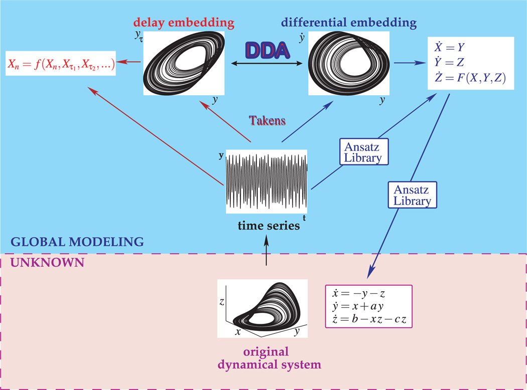
Figure 1 illustrates the connections of DDA to nonlinear dynamics and global modeling. In nonlinear time series analysis, a single variable measurement (the blue box in Figure 1) comes from an unknown nonlinear dynamical system (pink box in Figure 1). In Figure 1 the Rössler system (Rössler, 1976) is used for illustration. A general existence theorem for embeddings in an Euclidean space was given by Whitney (1936). A generic map from an n-dimensional manifold to a 2n + 1 dimensional Euclidean space is an embedding. Whitney’s theorem implies that each state can be identified uniquely by a vector of 2n + 1 measurements, thereby reconstructing the phase space. This theorem is the basis for the embedding theorems of Packard et al. (1980) and Takens (1981) for reconstruction of an attractor from single time series measurements. Takens proved that instead of 2n + 1 generic signals, the time-delayed versions [y(t), y(t − τ), y(t − 2τ), …, y(t − nτ)] or the successive derivatives of one generic signal would suffice to embed the n-dimensional manifold. Although the reconstruction preserves the invariant dynamical properties of the dynamical system, the embedding theorems provide no tool to reconstruct the original dynamical system in the original phase space from the single measurement or the embedding.

Figure 1.

Delay differential analysis (DDA) and global modeling.

The Ansatz Library is a tool to reconstruct a general system from a single measurement that contains the original dynamical system as a subset (Lainscsek, 1999, 2011; Lainscsek, Letellier, & Gorodnitsky, 2003; Lainscsek, Letellier, & Schürrer, 2001). For example, for the Rössler system (Röossler, 1976),

$$ẋ=a_{1,2}y+a_{1,3}z$$

$$ẏ=a_{2,1}x+a_{2,2}y$$

$$ż=a_{3,0}+a_{3,3}z+a_{3,6}xz,$$ (2.1)

the standard form (or the functional form of the differential embedding) is

$$Ẋ=Y,$$

$$Ẏ=Z,$$

$$Ż=F(X,Y,Z),$$ (2.2)

where X = x₂ and its successive derivatives define the new state-space variables X, Y, and Z. The function F(X, Y, Z) is explicitly

$$F(X,Y,Z)={\alpha }_1+X{\alpha }_2+X^2{\alpha }_3+Y{\alpha }_4+XY{\alpha }_5+Y^2{\alpha }_6+Z{\alpha }_7+XZ{\alpha }_8+YZ{\alpha }_9.$$ (2.3)

When we use the relations between the coordinates α_r of the differential embedding and the coordinates a_i,* the model of the Rössler system becomes

$${\dot{\phi }}_x=d^2\frac{1}{b}{a}_{1,2}y+d^3\frac{1}{b}\frac{1}{c}{a}_{1,3}{\phi }_z,$$

$$ẏ=b{a}_{2,1}{\phi }_x+d{a}_{2,2}y,$$

$${\dot{\phi }}_z=c{a}_{3,0}+d{a}_{3,3}{\phi }_z+b{a}_{3,6}{\phi }_x{\phi }_z,$$ (2.4)

where the functions φ_x = φ_x(x, z) and φ_z = φ_z(x, z) are generic linear independent functions of x and z (see Lainscsek et al., 2003, and Lainscsek, 2011, for details). The parameters b and c specify the structure of the parameter space a_i,* and d is an additional time-scaling parameter.

Such a reconstruction is possible only for simple dynamic systems with no noise and can be seen as the theoretical limit for global modeling. It also shows that measurements from the same dynamical system on different timescales (and consequently frequency shifted) can be identified as belonging to the same dynamical system. Further, the time-scaling parameter can be reconstructed as a separate parameter. This is consistent with Takens’s theorem, which does not specify the sampling rate.

Since real-world data are noisy and generally originate from highly complex dynamical systems, global modeling from data is in general not feasible. Often it is sufficient to detect dynamical differences between data classes and quantify the difference. DDA can distinguish between heart conditions in EKG (electrocardiography) data (Lainscsek & Sejnowski, 2013) and EEG data between Parkinson’s patients and control subjects (Lainscsek, Weyhenmeyer, Hernandez, Poizner, & Sejnowski, 2013). Dynamical differences can be detected and analyzed by combining derivative embeddings with delay embeddings as functional embeddings in the DDA framework.

DDA in the time domain can be related to frequency analysis as shown in the next section. In linear DDEs (Falbo, 1995), the estimated parameters and delays of a DDE relate to the frequencies of a signal, and in nonlinear DDEs, the estimated parameters are connected to higher-order statistical moments.

3 Functional Embedding as a Connection Between Nonlinear Dynamics and Frequency Analysis

3.1 Linear DDE and Frequency Analysis

Lainscsek & Sejnowski (2013) show that the linear DDE (Falbo, 1995),

$$ẋ=a{x}_{\tau },$$ (3.1)

where x_τ = x(t − τ), can be used to detect frequencies in the time domain: equation 3.1 with a harmonic signal with one frequency, x(t) = A cos(ωt + φ) can be written as

$$-aA\text{cos}(\omega (t-\tau )+\phi )-A\omega \text{sin}(t\omega +\phi )=0$$

$$\text{sin}(\omega t)(-aA\text{cos}(\phi )\text{sin}(\tau \omega )+aA\text{sin}(\phi )\text{cos}(\tau \omega )-A\omega \text{cos}(\phi ))+\text{cos}(\omega t)(-aA\text{sin}(\phi )\text{sin}(\tau \omega )-aA\text{cos}(\phi )\text{cos}(\tau \omega )-A\omega \text{sin}(\phi ))=0.$$ (3.2)

This equation has the solutions

$$\tau =\frac{(2n-1)\pi }{2\omega }\stackrel{\omega =2\pi f}{=}\frac{2n-1}{4f},a={(-1)}^n\omega ,n\in \mathbb{N}.$$ (3.3)

This means that the delays are inversely proportional to the frequency f and the coefficient a is directly proportional to the frequency. For linear DDEs,

$$ẋ=\sum _{k=1}^N{a}_k{x}_{{\tau }_k},$$ (3.4)

a special solution is a harmonic signal with 2N − 1 frequencies,

$$x(t)=\sum _{k=1}^{2N-1}{A}_k\text{cos}({\omega }_{k}t+{\phi }_k),$$ (3.5)

and

$${\tau }_i=\frac{\pi (2n-1)}{2{\omega }_j},n\in \mathbb{N},$$ (3.6)

where all delays τ_i are related to one of the frequencies. The expressions for the coefficients a are more complicated than in equation 3.3, and each of the coefficients a depends on all the frequencies in the signal.

Equation 3.1 can be expanded as a Yule-Walker equation (Yule, 1927;Walker, 1931; Boashash, 1995; Kadtke & Kremliovsky, 1999), $ẋx_{\tau }=a{x}_{\tau }^2$. Applying the expectation operator $\langle F(t)\rangle \equiv {\text{lim}}_{T\to \infty }(\frac{1}{T}{\int }_0^{T}F(t)\mathrm{d}\mathrm{t})$, we get

$$a=\frac{\langle ẋx_{\tau }\rangle }{\langle x_{\tau }^2\rangle }=\frac{\langle ẋx_{\tau }\rangle }{\langle x^2\rangle }.$$ (3.7)

For a harmonic signal with one frequency (this is a special solution of the linear DDE in equation 3.1; see Falbo, 1995, for details), x(t) = A cos(ωt + φ). This becomes:

$$\langle ẋx_{\tau }\rangle =-\frac{1}{2}\omega A^2\text{sin}(\omega \tau )$$

$$\Rightarrow a=-\omega \text{sin}(\omega \tau )$$ (3.8)

$$\langle x^2\rangle =\frac{1}{2}{A}^2$$

and for sin(ωτ) = ±1 the special solutions for a and τ are

$$\tau =\frac{(2n-1)\pi }{2\omega }\stackrel{\omega =2\pi f}{=}\frac{2n-1}{4f},a={(-1)}^n\omega ,$$ (3.9)

the same as in equation 3.3. For DDEs without explicit analytical solutions, Yule-Walker equations can be applied.

The numerator in equation 3.7 can be rewritten as delay derivatives of the autocorrelation function in the case of a bounded stationary signal,

$$\langle ẋx_{\tau }\rangle =\underset{T\to \infty }{\text{lim}}\frac{1}{T}{\int }_0^Tẋx_{\tau }dt=\underset{T\to \infty }{\text{lim}}\frac{1}{T}{[x{x}_{\tau }]}_0^T-\underset{T\to \infty }{\text{lim}}\frac{1}{T}{\int }_0^{T}x\frac{d{x}_{\tau }}{dt}dt==\underset{T\to \infty }{\text{lim}}\frac{1}{T}{\int }_0^{T}x\frac{d{x}_{\tau }}{d\tau }dt=\frac{d}{d\tau }\langle x{x}_{\tau }\rangle ;$$ (3.10)

therefore,

$$a=\frac{\langle ẋx_{\tau }\rangle }{\langle x^2\rangle }=\frac{\frac{d}{d\tau }\langle x{x}_{\tau }\rangle }{\langle x^2\rangle }.$$ (3.11)

Thus, the numerator in equation 3.11 is the delay derivative of the autocorrelation function 〈x x_τ〉. For a harmonic signal $x(t)={\sum }_{k=1}^N{A}_k\text{cos}({\omega }_{k}t+{\phi }_k)$ with N frequencies, it is $\langle x{x}_{\tau }\rangle =\frac{1}{2}{\sum }_{k=1}^N{A}_k^2\text{cos}({\omega }_k\tau )$ and is used for pitch detection (Boersma, 1993; Roads & Curtis, 1996).

The denominator 〈x²〉 will be used as frequency detector in the following way: Consider a signal

$$x(t)=\underset{𝒮}{\underbrace{\sum _{i=1}^N{A}_i\text{cos}({\omega }_{i}t+{\phi }_i)}}+\underset{𝒫}{\underbrace{D\text{cos}(\mathrm{\Omega }t+\varphi )}},$$ (3.12)

where 𝒮 is the signal under investigation and 𝒫 = D cos(Ωt + ϕ) is a probe signal. The expectation value $\langle x^2\rangle ={\text{lim}}_{T\to \infty }\frac{1}{T}{\int }_0^T{x}^2\mathrm{d}\mathrm{t}$ can be written in the form

$$\langle x^2\rangle =\langle {(𝒮+𝒫)}^2\rangle =\langle {𝒮}^2\rangle +2\langle 𝒮𝒫\rangle +\langle {𝒫}^2\rangle ,$$

$$\langle {𝒮}^2\rangle =\frac{1}{2}\sum _{i=1}^N{A}_i^2,$$

$$\langle {𝒫}^2\rangle =\frac{1}{2}{D}^2,$$

$$\langle 𝒮𝒫\rangle =\{\begin{array}{c}0\hfill \\ A_{i}D\text{cos}({\phi }_i-\varphi )\hfill \end{array}\text{for}\begin{array}{c}{\omega }_i\ne \mathrm{\Omega }\hfill \\ {\omega }_i=\mathrm{\Omega }\hfill \end{array}.$$ (3.13)

The term 〈𝒮𝒫〉 = 〈𝒮 D cos(Ωt + ϕ)〉 combines ℛ = 〈𝒮 cos(Ωt)〉 and ℐ = 〈𝒮 sin(Ωt)〉 used in discrete frequency analysis.

3.1.1 Time Domain Spectrum

Let the amplitude of the probe signal be D = 1 (arbitrary parameter). Then one way to define the time domain spectrum (TDS) is

$$L(\mathrm{\Omega })=\underset{\varphi }{\text{max}}(\langle x^2\rangle -\langle {𝒮}^2\rangle -\frac{1}{2}).$$ (3.14)

L(Ω) is zero for frequencies Ω that are not part of the signal 𝒮 and equal to the amplitude A_i of a frequency $f_i=\frac{{\omega }_i}{2\pi }$ if Ω = ω_i, which follows directly from $\langle x^2\rangle =\langle {𝒮}^2\rangle +\frac{1}{2}+A_i\text{cos}({\phi }_i-\varphi )$. The amplitude A_i is always positive, and cos(φ_i − ϕ) ranges between −1 and 1 with a maximum when ϕ = φ_i. For a given signal 𝒮, we loop over a range of ϕ values between 0 and 2π and take the maximal value of $\langle x^2\rangle -\langle {𝒮}^2\rangle -\frac{1}{2}=A_i$. The value ϕ that maximizes cos(φ_i − ϕ) is then equal to the phase φ_i. Therefore, this simultaneously detects the amplitudes A_i and their phases φ_i in a signal. This method can detect frequencies and couplings only at lower than half the sampling rate since $\mathrm{\Omega }=\frac{2\pi f}{f_s}$, where f_s is the sampling rate, in cos(Ωt + ϕ) with the time t given in time steps needs to be smaller than π. This is the same as the Nyquist frequency limit for traditional methods (Nyquist, 1928).

3.1.2 Comparison to the Goertzel Algorithm and Discrete Frequency Analysis

In discrete frequency analysis for a signal $𝒮(t)={\sum }_{i=1}^N{A}_i\text{cos}({\omega }_{i}t+{\phi }_i)$, the expectation values ℛ = 〈𝒮 cos(Ωt)〉 and ℐ = 〈𝒮 sin(Ωt)〉 are computed. ℛ and ℐ are nonzero only if Ω is contained in the signal. The amplitude of that frequency is then $A_i\stackrel{\mathrm{\Omega }={\omega }_i}{=}4\sqrt{{ℛ}^2+{ℐ}^2}$, and the phase is ${\phi }_i={\text{tan}}^{-1}\frac{ℐ}{ℛ}$. The Goertzel algorithm (Goertzel, 1958; Jacobsen & Lyons, 2003) is the numerical implementation of this principle and gives the same results as the computation of the TDS.

The TDS L(Ω) differs from discrete frequency analysis in two ways. First, D cos(Ωt + ϕ) is multiplied with the signal 𝒮 instead of cos(Ωt). Second, only 〈𝒮𝒫〉 = 〈𝒮 D cos(Ωt + ϕ)〉 is computed instead of ℛ = 〈𝒮 cos(Ωt)〉 and ℐ = 〈𝒮 sin(Ωt)〉. Amplitudes and phases are extracted from 〈𝒮𝒫〉 instead of $A_i\stackrel{\mathrm{\Omega }={\omega }_i}{=}2\sqrt{{ℛ}^2+{ℐ}^2}$ and ${\phi }_i={\text{tan}}^{-1}\frac{ℐ}{ℛ}$. An advantage of L(Ω) is that it can be more easily expanded to the computation of higher-order spectra (e.g., the bispectrum).

3.2 Nonlinear DDE and Bispectral Analysis

3.2.1 Quadratic Phase and Frequency Couplings

Frequency components do not always appear completely independent of one another. Nonlinear interactions of frequencies and their phases (e.g., quadratic phase coupling) cannot be detected by a power spectrum—the Fourier transform of the autocorrelation function (second-order cumulant)—since phase relationships and frequency couplings of signals are lost. Such couplings are usually detected by bispectral analysis (Tukey, 1953; Kolmogorov & Rozanov, 1960;Leonov & Shiryeav, 1959; Rosenblatt & Van Ness, 1965; Brillinger & Rosenblatt, 1967; Swami, 2003; Mendel, 1991; Fackrell & McLaughlin, 1995). The bispectrum or bispectral density is the Fourier transform of the third-order cumulant (bicorrelation function).

Consider the signal x(t) = A₁ cos(ω₁t + φ₁) + A₂ cos(ω₂t + φ₂), which is passed through a quadratic nonlinear system h(t) = bx²(t) where b is a nonzero constant. The output of the system will include the harmonic components: (2ω₁, 2φ₁), (2ω₂, 2φ₂), (ω₁ + ω₂, φ₁ + φ₂), and (ω₁ − ω₂, φ₁ − φ₂). These phase relations are called quadratic phase coupling (QPC) in general and quadratic frequency coupling (QFC) when the phases are zero (φ₁ = φ₂ = 0). For the signal x(t) = cos(ω₁t) + cos(ω₂t) + cos(ω₃t), QFC occurs when ω₃ is a multiple of one of the frequencies or of the sum or difference of the two frequencies.

The third-order cumulant is C₃(τ₁, τ₂) = 〈x(t)x(t − τ₁)x(t − τ₂)〉, and the traditional bispectrum is the double Fourier transform of C₃,

$$B_x(f_1,f_2)={ℱ}^{\star }(f_1+f_2)ℱ(f_1)ℱ(f_2),$$ (3.15)

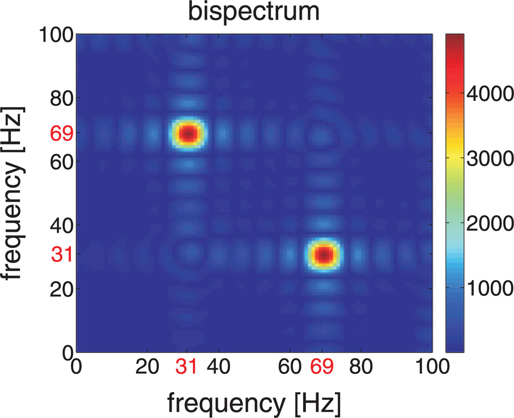
where ℱ(f) is the Fourier transform of x(t). An example is given in Figure 2.

Figure 2.

Bispectrum magnitude (see equation 3.15) for the signal $𝒮={\sum }_{i=1}^3{A}_i\text{cos}({\omega }_{i}t+{\phi }_i)+\text{cos}(({\omega }_1+{\omega }_3)t+({\phi }_1+{\phi }_3))$ with the frequencies, amplitudes, and phases listed in Table 1.

3.2.2 Nonlinear DDE

The simplest nonlinear DDE,

$$ẋ=a{x}_{\tau }^2,$$ (3.16)

where x_τ = x(t − τ), extends linear spectral analysis to quadratic coupling analysis or bispectral analysis. This equation can be solved in the same way as the linear DDE:

$$a=\frac{\langle ẋx_{\tau }^2\rangle }{\langle x_{\tau }^4\rangle }=\frac{\langle ẋx_{\tau }^2\rangle }{\langle x^4\rangle }.$$ (3.17)

For a harmonic signal with three frequencies x(t) = A₁ cos(ω₁ t + φ₁) + A₂ cos(ω₂ t + φ₂) + A₃ cos(ω₃ t + φ₃), the coefficient a is nonzero only if there is quadratic coupling between the frequencies: ω₃ = ω₁ ± ω₂, 2ω₁, 2ω₂, $\frac{{\omega }_1}{2}$, or $\frac{{\omega }_2}{2}$. Only the numerator $\langle ẋx_{\tau }^2\rangle$ contains quadratic coupling information and can be rewritten for a bounded stationary signal:

$$\langle ẋx_{\tau }^2\rangle =\underset{T\to \infty }{\text{lim}}\frac{1}{T}{\int }_0^Tẋx_{\tau }^{2}dt=\underset{T\to \infty }{\text{lim}}\frac{1}{T}{[x{x}_{\tau }^2]}_0^T-\underset{T\to \infty }{\text{lim}}\frac{1}{T}{\int }_0^{T}x\frac{d{x}_{\tau }^2}{dt}dt==\underset{T\to \infty }{\text{lim}}\frac{1}{T}{\int }_0^{T}x\frac{d{x}_{\tau }^2}{d\tau }dt=\frac{d}{d\tau }\langle x{x}_{\tau }^2\rangle .$$ (3.18)

The denominator in equation 3.17 is a constant independent of up to quadratic couplings in the signal. Therefore equation 3.17 can be rewritten as

$$a\langle x^4\rangle =\langle ẋx_{\tau }^2\rangle$$

$$\frac{d}{d\tau }\langle x{x}_{\tau }^2\rangle =\text{const}.$$ (3.19)

For $x(t)={\sum }_{i=1}^{\infty }{A}_i\text{cos}({\omega }_{i}t+{\phi }_i)+A_{j,k}\text{cos}(({\omega }_j+{\omega }_k)t+{\phi }_j+{\phi }_k)$, the expectation value is

$$\langle x{x}_{\tau }^2\rangle =\frac{1}{2}{A}_j{A}_k{A}_{j,k}(\text{cos}({\omega }_j\tau )+\text{cos}({\omega }_k\tau )+\text{cos}(({\omega }_j+{\omega }_k)\tau )).$$ (3.20)

Therefore, $\langle x{x}_{\tau }^2\rangle$ is zero for a signal without QFC (A_j,k = 0) and nonzero if there is QFC in the signal. Without loss of generality, the delay τ can be set to zero in equation 3.20 and $\langle x{x}_{\tau }^2\rangle \stackrel{\tau =0}{=}\langle x^3\rangle =\frac{3}{2}{A}_j{A}_k{A}_{j,k^{·}}\langle x^3\rangle$, and the coefficient a of the nonlinear DDE in equation 3.16 is then nonzero only if QFC is present in the signal (A_j,k ≠ 0) and can be used as a bispectral detector. 〈x³〉 can detect the presence or absence of QFC but not the frequencies involved. To determine the frequencies, the time domain bispectrum is introduced.

3.2.3 Time Domain Bispectrum

To determine the frequencies of QFC, consider a signal

$$x(t)=𝒮+𝒫,$$

$$𝒮=\sum _{i=1}^N{A}_i\text{cos}({\omega }_{i}t+{\phi }_i)+A_{j,k}\text{cos}(({\omega }_j+{\omega }_k)t+({\phi }_j+{\phi }_k)),$$

$$𝒫=D\text{cos}(\mathrm{\Omega }t+\varphi ),$$ (3.21)

where 𝒮 is the signal under investigation and 𝒫 = D cos(Ωt + ϕ) is a probe signal. The frequencies f_j and f_k are coupled. 〈x³〉 is then

$$\langle x^3\rangle =\langle {𝒮}^3\rangle +3\langle {𝒮}^2𝒫\rangle +3\langle 𝒮{𝒫}^2\rangle +\langle {𝒫}^3\rangle ,$$

$$\langle {𝒮}^3\rangle =\frac{3}{2}{A}_{j,k}{A}_j{A}_k,$$

$$\langle {𝒮}^2𝒫\rangle =\{\begin{array}{cc}\frac{1}{2}{A}_j{A}_{k}D\text{cos}(\varphi -{\phi }_j\mp {\phi }_k)\hfill & \mathrm{\Omega }={\omega }_j\pm {\omega }_k\hfill \\ \frac{1}{2}{A}_k{A}_{j,k}D\text{cos}(\varphi -{\phi }_j)\hfill & \mathrm{\Omega }={\omega }_j\hfill \\ \frac{1}{4}{A}_i^{2}D\text{cos}(\varphi -2{\phi }_i)\hfill & \mathrm{\Omega }=2{\omega }_i\hfill \\ 0\hfill & \mathrm{\Omega }\text{otherwise}\hfill \end{array},$$

$$\langle 𝒮{𝒫}^2\rangle =\{\begin{array}{cc}\frac{1}{4}{A}_i{D}^2\text{cos}(2\varphi -{\phi }_i)\hfill & \mathrm{\Omega }=\frac{{\omega }_i}{2}\hfill \\ 0\hfill & \mathrm{\Omega }\text{otherwise}\hfill \end{array},$$

$$\langle {𝒫}^3\rangle =0.$$ (3.22)

The term 〈𝒮 𝒫²〉 is nonzero only when Ω̃ = 2Ω = ω_i. It therefore can be used as an alternative definition of the time domain spectrum TDS in equation 3.14:

$$L(\tilde{\mathrm{\Omega }})=\underset{\varphi }{\text{max}}\langle 𝒮{𝒫}^2\rangle .$$ (3.23)

To define the time domain bispectrum (TDB), we set in our analysis D = 1:

$$B(\mathrm{\Omega })=L(\tilde{\mathrm{\Omega }})\cdot \underset{\varphi }{\text{max}}\langle {𝒮}^2𝒫\rangle .$$ (3.24)

The expression max 〈𝒮² 𝒫〉 is zero for frequencies Ω that are not coupled and non-zero according to equation 3.22 for the coupling frequencies ω_j ± ω_k, ω_j, ω_k, and 2ω_i. To get only a nonzero expression for ω_j + ω_k, ω_j, and ω_k, we use L(Ω̃) in equation 3.24 to filter out 2ω_i.

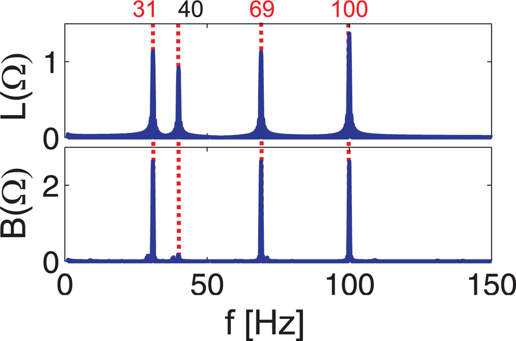
Note that unlike the bispectrum, which is a function of two frequencies (see Figure 2), the TDB is a function of a single frequency. In Figure 3, the TDB is shown for the same signal used to illustrate the traditional bispectrum in Figure 2. Note that the 40 Hz component, which is not coupled, is absent in both the TBS and the bispectrum but is present in the TDS.

Figure 3.

Time domain spectrum TDS L(Ω) and time domain bispectrum TDB B(Ω) for the signal $𝒮={\sum }_{i=1}^3{A}_i\text{cos}({\omega }_{i}t+{\phi }_i)+\text{cos}(({\omega }_1+{\omega }_3)t+({\phi }_1+{\phi }_3))$ with the frequencies, amplitudes, and phases listed in Table 1.

3.3 General Nonlinear DDE as Generalized Nonlinear Spectral Tool

Combining linear and nonlinear terms in a DDE makes all coefficients nonlinear. If we, for example, combine the DDEs of sections 3.1 and 3.2,

$$ẋ=a_1{x}_{\tau }+a_2{x}_{\tau }^2,$$ (3.25)

the solution can be written as

$$a_1=\frac{\langle x_{\tau }^4\rangle \langle x_{\tau }ẋ\rangle -\langle x_{\tau }^3\rangle \langle x_{\tau }^2ẋ\rangle }{\langle x_{\tau }^2\rangle \langle x_{\tau }^4\rangle -{\langle x_{\tau }^3\rangle }^2}=\frac{\langle x^4\rangle \frac{d}{d\tau }\langle x_{\tau }x\rangle -\langle x^3\rangle \frac{d}{d\tau }\langle x_{\tau }^{2}x\rangle }{\langle x^2\rangle \langle x^4\rangle -{\langle x^3\rangle }^2},$$

$$a_2=\frac{\langle x_{\tau }^2\rangle \langle x_{\tau }^2ẋ\rangle -\langle x_{\tau }^3\rangle \langle x_{\tau }ẋ\rangle }{\langle x_{\tau }^2\rangle \langle x_{\tau }^4\rangle -{\langle x_{\tau }^3\rangle }^2}=\frac{\langle x^2\rangle \frac{d}{d\tau }\langle x_{\tau }^{2}x\rangle -\langle x^3\rangle \frac{d}{d\tau }\langle x_{\tau }x\rangle }{\langle x^2\rangle \langle x^4\rangle -{\langle x^3\rangle }^2}.$$ (3.26)

The coefficient a₁ as well as the coefficient a₂ contain both linear and nonlinear statistical moments. The moments and coefficients for combinations of sinusoids are given in Table 2 with and without couplings.

Table 2.

Moments and Coefficients of Equations 3.25 and 3.26.

	Couplings Present	No Couplings
	$x(t)={\sum }_{k=1}^N{A}_k\text{cos}({\omega }_{k}t+{\phi }_k)+{\sum }_{i=1}^N{\sum }_{j=i+1}^N(A_{i,j}\text{cos}(({\omega }_i+{\omega }_j)t+({\phi }_i+{\phi }_j)))$	$x(t)={\sum }_{k=1}^N{A}_k\text{cos}({\omega }_{k}t+{\phi }_k)$
〈x2〉	Const.	Const.
〈x3〉	Const.	0
〈x4〉	Const.	Const.
〈xτ x〉	f (ωi, j, k, τ)	f (ωk, τ)
$\langle x_{\tau }^{2}x\rangle$	f (ωi, j, k, τ)	0
a1	f (ωi, j, k, τ)	f (ωk, τ)
a2	f (ωi, j, k, τ)	0

Note: The coefficient a₂ is nonzero only if QFC is present in the data.

3.3.1 Example 1: Data with No Couplings

To explore the properties of equation 3.26, we start with a harmonic signal with four independent frequencies and no couplings:

$$x(t)=\sum _{k=1}^4{A}_k\text{cos}({\omega }_{k}t+{\phi }_k).$$ (3.27)

Using equation 3.26, we get for the two coefficients,

$$a_1=\frac{3}{16}(A^{(1)}+4A_2^2{A}_3^2+4A_4^2{A}_3^2+4A_2^2{A}_4^2)\sum _{k=1}^4{A}_k^2{\omega }_k\text{sin}\left(\tau {\omega }_k\right),$$

$$a_2=0,$$ (3.28)

where $A^{(1)}=A_1^4+A_2^4+A_3^4+A_4^4+4A_1^2(A_2^2+A_3^2+A_4^2)$. The nonlinear coefficient a₂ vanishes in this case.

3.3.2 Example 2: Data with Couplings

Replace the fourth term in equation 3.27 with a coupling frequency,

$$x(t)=\sum _{k=1}^3{A}_k\text{cos}({\omega }_{k}t)+A_4\text{cos}(({\omega }_2+{\omega }_3)t+({\phi }_2+{\phi }_3)).$$ (3.29)

The two coefficients are:

$$a_1=\frac{3}{16}((A^{(1)}+4A_2^2{A}_3^2+4A_4^2{A}_3^2+4A_2^2{A}_4^2)A_1^2{\omega }_1\text{sin}(\tau {\omega }_1)+(4A_2^2{A}_3^2+A^{(1)})(A_2^2{\omega }_2\text{sin}(\tau {\omega }_2)+A_3^2{\omega }_3\text{sin}(\tau {\omega }_3))+4A_4^2(A_2^4{\omega }_2\text{sin}(\tau {\omega }_2)+A_3^4{\omega }_3\text{sin}(\tau {\omega }_3))+A_4^2({\omega }_2+{\omega }_3)(4A_2^2{A}_4^2+4A_3^2{A}_4^2+A^{(1)})(\text{sin}(\tau {\omega }_2)\text{cos}(\tau {\omega }_3)+\text{sin}(\tau {\omega }_3)\text{cos}(\tau {\omega }_2)),$$

$$a_2=\frac{1}{4}{A}^{(2)}(-3A_1^2{\omega }_1\text{sin}(\tau {\omega }_1)+(A_1^2-2A_2^2+A_3^2+A_4^2){\omega }_2\text{sin}(\tau {\omega }_2)+(A_1^2+A_2^2-2A_3^2+A_4^2){\omega }_3\text{sin}(\tau {\omega }_3)+(A_1^2+A_2^2+A_3^2-2A_4^2)({\omega }_2+{\omega }_3)(\text{sin}(\tau {\omega }_2)\text{cos}(\tau {\omega }_3)+\text{sin}(\tau {\omega }_3)\text{cos}(\tau {\omega }_2))),$$ (3.30)

where $A^{(1)}=A_1^4+A_2^4+A_3^4+A_4^4+4A_1^2(A_2^2+A_3^2+A_4^2)$ and A⁽²⁾ = A₂A₃A₄.

Equation 3.25 is therefore a QFC detector. For any signal without QFC, the coefficient a₂ will vanish. The detection of nonlinear couplings in the data is important in underwater acoustics (Nikias & Raghuver, 1987).

4 Sparse Data

Real-world data often contain data segments that cannot be used for the analysis, such as artifacts in electroencephalography (EEG) data. Equation 3.14 can nonetheless be used even when many data points are missing. For a sparse signal x(T), where T is the vector of times for which the signal is good, the probe signal cos(ΩT + ϕ) can be used to detect the spectrum or any higher-order spectra. Equation 3.12 can be modified as

$$x(T)=\underset{𝒮}{\underbrace{\sum _{i=1}^N{A}_i\text{cos}({\omega }_{i}T+{\phi }_i)}}+\underset{𝒫}{\underbrace{\text{cos}(\mathrm{\Omega }T+\varphi )}},$$ (4.1)

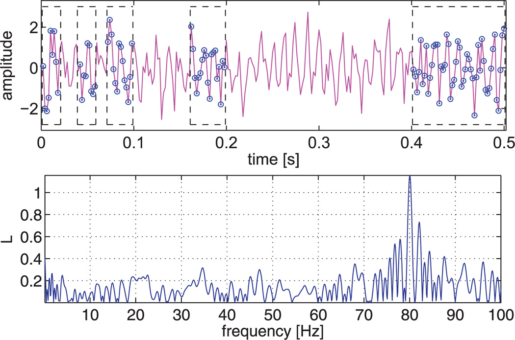
where T is a sparse time vector. The upper plot in Figure 4 shows an example where only a few data points of a signal were used. Those data and their time points were then used to compute the TDS using equation 3.14. The TDS for these sparse data is shown in the lower plot of Figure 4. Note that the sparse data have to satisfy the restrictions of the Nyquist theorem (Nyquist, 1928). Equation 3.24 can be used for the bispectrum of sparse data in the same way.

Figure 4.

Frequency detection from sparse data. Only 101 data points circled from a signal 𝒮 = cos(2π ft) with f = 80 Hz and a sampling rate of 500 Hz and added white noise (SNR = 0 dB) (upper plot) were used to detect the frequency f (lower plot).

5 Cross-Trial Spectrogram and Bispectrogram

The same method can be used when very short segments of data need to be analyzed and there are multiple trials of the same experiment, as in event-related potential (ERP) analysis (Davis, 1939; Davis & Davis, 1936;Sutton, Braren, Zubin, & John, 1965; Luck, 2014). There are two different ways to define a cross-trial spectrogram (CTS). The first assumes that there is cross-trial phase coherence; the second does not.

5.1 Phase Coherence Across Trials

The first method assumes phase coherence across trials. Consider a signal x₁(T₁), x₂(T₂), …, x_n(T_n) where all time series x_i(T_i) are centered around the same event (e.g., a stimulus S for EEG data). Then all time vectors T_i can be considered equal and the signal can be concatenated into a single vector, x₁(T), x₂(T), …, x_n (T); L_i(Ω) is computed for this single vector. For a short data window that would be too short for spectral analysis, the data of all trials can be combined and the spectrum can be computed by using a probe signal with a time vector that consists of n repetitions of the time vector T for n data segments. In this manner, a cross-trial spectrogram can be computed by using short sliding windows when there is some phase coherence in the relevant frequencies.

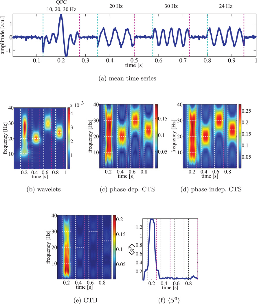
To test this, we generated a signal 𝒮_i = 𝒲_i +Y_i, where 𝒲 is white noise andY_i are short-phase coherent (phases varied in a range from0 to π for each trial) data segments of 150 ms (t =[126, 279] ms, [350, 500] ms, [576, 726] ms, and [800, 950] ms). The frequencies in the first segment are 10, 20, and 30 Hz (QFC); the single frequencies in the following three segments are 20, 30, and 24 Hz, respectively. Twenty-one second data segments (i = 1, 2, …, 20) at a sampling rate of 500 Hz were generated to simulate data from repeated trials in an experiment.

Figure 5a shows the mean signal of these 20 trials. Sliding windows of 100 ms (50 data points) with a window shift of 10 ms (5 data points) were used to compute the CTS in Figure 5c. This CTS was compared with traditional Morlet wavelet analysis (Mallat, 2008) in Figure 5b.

Figure 5.

Cross-trial spectrogram (CTS) of phase-coherent simulated data with white noise. Four segments of noisy short signals of 10, 20, 24, and 30 Hz with some phase coherence added to the data. Horizontal white dashed lines indicate frequencies present in each segment. (a) Mean over the 20 trials. (b)Wavelet spectrogram. (c) Phase-dependent CTS. (d) Phase-independent CTS. (e) Bispectrogram CTB. (f) bispectral detector $\overline{|\langle S^3\rangle |}$.

In a companion paper (Lainscsek et al., 2015), we apply this method to EEG data.

5.2 No Phase Coherence Across Trials

The second cross-trial method does not assume phase coherence across trials and is defined by computing L_i(Ω) in equation 3.14 for each trial using sliding windows and then averaging over the 20 spectra L_i(Ω) (i = 1, 2, …, 20).

Figure 5c shows the CTS assuming phase coherence in the signal, and Figure 5d shows the phase-independent CTS. All three methods identified the frequencies correctly, and both CTS methods produce similar results (the correlation coefficient between Figures 5c and 5d is 0.96).

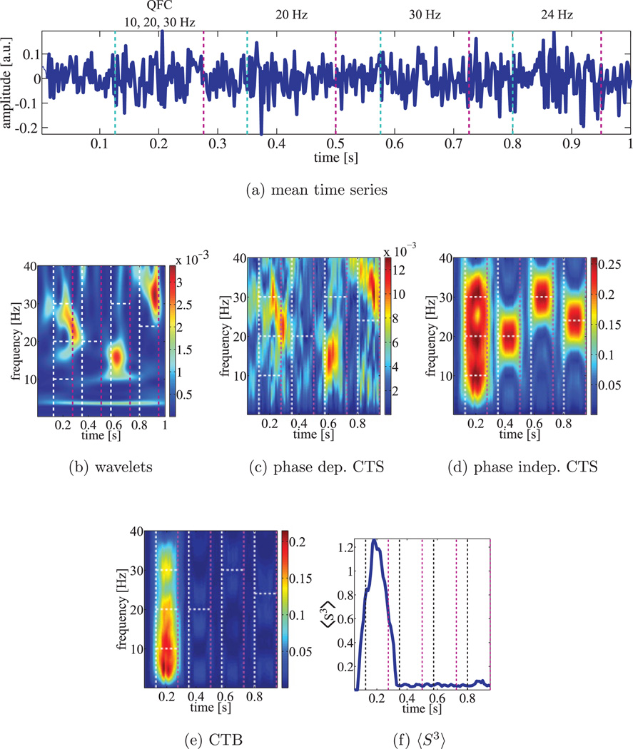
The same experiment was repeated for completely phase-randomized data segments Y_i. Figure 6a shows the mean of the data, Figure 6b the traditional Morlet wavelet analysis, Figure 6c the CTS assuming phase coherence, and Figure 6d the phase-independent CTS. Only the phase-independent CTS can identify the frequencies correctly. The correlation coefficient between Figures 6c and 6d drops to 0.15. Therefore, the correlation coefficient between the phase-dependent CTS and the phase independent CTS can be used to quantify the amount of phase coherence.

Figure 6.

Cross-trial spectrogram (CTS) of nonphase-coherent simulated data with white noise. Four segments of noisy short signals of 10, 20, 24, and 30 Hz with no phase coherence added to the data. (a) The mean over the 20 trials. (b) The wavelet spectrogram. (c) The phase-dependent CTS. (d) The phase-independent CTS. (e) The bispectrogram CTB. (f) The bispectral detector $\overline{|\langle S^3\rangle |}$.

If multiple channels are available, data from different channels or different trials can be combined. Such cross-trial spectra are different from the cross-spectral density (Bracewell, 1965; Papoulis, 1962) based on the cross-correlation between two signals.

Since the TDB in equation 3.24 is a function of a single frequency (one-dimensional plot instead of a two-dimensional plot for the traditional bispectrum), the TDB bispectrogram can be obtained in the same way as a spectrogram. The single-trial, cross-trial, or cross-channel TDS (or spectrogram) can be extended to a single-trial, cross-trial, or cross-channel bispectrogram (CTB) by replacing L(Ω) with B(Ω). The bispectral detector 〈S³〉 in Figures 5f and 6f indicates the presence of QFC in the first data segment, and CTB in Figures 5e and 6e show couplings in the first data segment with the three coupled frequencies 10, 20, and 30 Hz (10 + 20 = 30) present. There is no frequency coupling in other data segments.

6 Discussion

Delay differential analysis is a nonlinear dynamical time series classification and detection tool based on embedding theory. It combines aspects of delay and differential embeddings in the form of delay differential equations (DDEs), which can detect distinguishing dynamical information in data. We focused here on the connection between traditional frequency analysis and linear DDEs and between higher-order statistics and nonlinear DDEs.

We introduced a new set of time domain tools to analyze the frequency content and frequency coupling in signals: the time domain spectrum(TDS), the time domain bispectrum (TDB), the time domain cross-trial (or cross-channel) spectrogram (CTS), and the time domain cross-trial (or cross-channel) bispectrogram (CTB). In addition, the CTS has a phase-dependent and a phase-independent realization.

These new time domain methods are complementary to traditional frequency domain methods and have several advantages:

• Because these new DDA spectral methods use time itself as a variable, they can be applied cross-trial and on sparse data.

• DDA can be applied to short data segments and therefore has an improved time resolution compared with the fast Fourier transform, which was developed to be computationally fast on longer time series.

• Because some numerical components of $\frac{1}{f}$ noise are not present, the new time domain spectrogram introduced here does not need normalization across frequencies. The sources of $\frac{1}{f}$ noise will be discussed elsewhere.

• DDA is noise insensitive (Lainscsek, Weyhenmeyer et al. (2013)). Short data segments from the Rössler system with a signal-to-noise ratio between 10 dB and −5 dB (more noise than data) were well separated. This separation was also correlated to the dynamical bifurcation parameter and generalized well to new data.

• DDA can discriminate dynamical differences in data classes using a small set of features, thus avoiding overfitting. With DDA, only five features are sufficient for many applications, whereas traditional methods often rely on many more features. The goal is not to achieve the most predictive model but the most discriminative model.

• Higher-order nonlinearities are intrinsically included in DDA, in comparison with nonlinear extensions of spectral analysis, which are not straightforward and are complicated.

There are many applications of DDA, including classification of electrocardiograms (Lainscsek & Sejnowski, 2013), electroencephalograms (Lainscsek, Hernandez, Weyhenmeyer, Sejnowski, & Poizner, 2013), speech (Gorodnitsky&Lainscsek, 2004), and sonar time series (Lainscsek & Gorodnitsky, 2003).

Table 1.

Frequencies f_i, Amplitudes A_i, and Phases φ_i for the Numerical Experiments Shown in Figures 2 and 3.

i	fi	Ai	φi
1	31	1.14	0.53
2	40	0.92	1.14
3	69	1.13	0.09

References

- Boashash B. Higher-order statistical signal processing. Hoboken, NJ: Wiley; 1995. [Google Scholar]
- Boersma P. Accurate short-term analysis of the fundamental frequency and the harmonics-to-noise ratio of a sampled sound. Proceedings 17 of the Institute of Phonetic Sciences, University of Amsterdam. 1993:97–110. [Google Scholar]
- Bracewell R. The Fourier transform and its applications. New York: McGraw-Hill; 1965. [Google Scholar]
- Brillinger D, Rosenblatt M. Asymptotic theory of estimates of kth order spectra. In: Harris B, editor. Spectral analysis of time series. Hoboken, NJ: Wiley; 1967. pp. 153–188. [DOI] [PMC free article] [PubMed] [Google Scholar]
- Chan Y, Langford R. Spectral estimation via the high-order Yule-Walker equations. IEEE Transactions on Acoustics, Speech and Signal Processing. 1982;30(5):689–698. [Google Scholar]
- Davis H, Davis P. Action potentials of the brain: In normal persons and in normal states of cerebral activity. Archives of Neurology and Psychiatry. 1936;36(6):1214–1224. [Google Scholar]
- Davis PA. Effects of acoustic stimuli on the waking human brain. Journal of Neurophysiology. 1939;2(6):494–499. [Google Scholar]
- Fackrell J, McLaughlin S. Quadratic phase coupling detection using higher order statistics. Proceedings of the IEE Colloquium on Higher Order Statistics. 1995:9. N.p. [Google Scholar]
- Falbo CE. Proceedings of the Joint Meeting of the Northern and Southern California Sections of the MAA. San Luis Obispo, CA: 1995. Analytic and numerical solutions to the delay differential equation y′ (t) = αy(t − δ) N.p. [Google Scholar]
- Fourier J. Théorie analytique de la chaleur. Paris: Chez Firmin Didot; 1822. [Google Scholar]
- Goertzel G. An algorithm for the evaluation of finite trigonometric series. American Mathematical Monthly. 1958;65(1):34–35. [Google Scholar]
- Gorodnitsky I, Lainscsek C. Machine emotional intelligence: A novel method for spoken affect analysis. In: Triesch J, Jebara T, editors. Proc. Intern. Conf. on Development and Learning ICDL 2004. San Diego, CA: UCSD Institute for Neural Computation; 2004. [Google Scholar]
- Hjorth B. EEG analysis based on time domain properties. Electroencephalography and Clinical Neurophysiology. 1970;29(3):306–310. doi: 10.1016/0013-4694(70)90143-4. [DOI] [PubMed] [Google Scholar]
- Jacobsen E, Lyons R. The sliding DFT. IEEE Signal Processing Magazine. 2003;20(2):74–80. [Google Scholar]
- Kadtke J, Kremliovsky M. Estimating dynamical models using generalized correlation functions. Physics Letters A. 1999;260(3–4):203–208. [Google Scholar]
- Kolmogorov A, Rozanov Y. On strong mixing conditions for gaussian processes. Theor. Prob. Appl. 1960;5:204–208. [Google Scholar]
- Lainscsek C. Doctoral dissertation. Technische Universität Graz; 1999. Identification and global modeling of nonlinear dynamical systems. [Google Scholar]
- Lainscsek C. Nonuniqueness of global modeling and time scaling. Phys. Rev. E. 2011;84:046205. doi: 10.1103/PhysRevE.84.046205. [DOI] [PubMed] [Google Scholar]
- Lainscsek C, Gorodnitsky I. Oceans 2003: Celebrating the past … Teaming toward the future. Vol. 2. Piscataway, NJ: Marine Technology Society/IEEE; 2003. Characterization of various fluids in cylinders from dolphin sonar data in the interval domain; pp. 629–632. [Google Scholar]
- Lainscsek C, Hernandez ME, Poizner H, Sejnowski TJ. Delay differential analysis of electroencephalographic data. Neural Computation. 2015;27(3):615–627. doi: 10.1162/NECO_a_00656. [DOI] [PMC free article] [PubMed] [Google Scholar]
- Lainscsek C, Hernandez ME, Weyhenmeyer J, Sejnowski TJ, Poizner H. Non-linear dynamical analysis of EEG time series distinguishes patients with Parkinson’s disease from healthy individuals. Frontiers in Neurology. 2013;4(200) doi: 10.3389/fneur.2013.00200. [DOI] [PMC free article] [PubMed] [Google Scholar]
- Lainscsek C, Letellier C, Gorodnitsky I. Global modeling of the Rössler system from the z-variable. Physics Letters A. 2003;314:409–427. [Google Scholar]
- Lainscsek C, Letellier C, Schürrer F. Ansatz library for global modeling using a structure selection. Physical Review E. 2001;64:016206. doi: 10.1103/PhysRevE.64.016206. [DOI] [PubMed] [Google Scholar]
- Lainscsek C, Sejnowski T. Electrocardiogram classification using delay differential equations. Chaos. 2013;23(2):023132. doi: 10.1063/1.4811544. [DOI] [PMC free article] [PubMed] [Google Scholar]
- Lainscsek C, Weyhenmeyer J, Hernandez M, Poizner H, Sejnowski T. Non-linear dynamical classification of short time series of the Rössler system in high noise regimes. Frontiers in Neurology. 2013;4(182) doi: 10.3389/fneur.2013.00182. [DOI] [PMC free article] [PubMed] [Google Scholar]
- Leonov V, Shiryeav A. On a method of calculation of semi-invariants. Theor. Prob. Appl. 1959;4:319–329. [Google Scholar]
- Luck S. An introduction to the event-related potential technique. 2nd ed. Cambridge, MA: MIT Press; 2014. [Google Scholar]
- Mallat S. A wavelet tour of signal processing: The sparse way. 3rd ed. Orlando, FL: Academic Press; 2008. [Google Scholar]
- Mendel J. Tutorial on higher-order statistics (spectra) in signal processing and system theory: Theoretical results and some applications. Proc. IEEE. 1991;79:278–305. [Google Scholar]
- Nikias C, Raghuver M. Bispectrum estimation: A digital signal processing framework. Proc. IEEE. 1987;75:869–891. [Google Scholar]
- Nyquist H. Certain topics in telegraph transmission theory. Trans. AIEE. 1928;47:617–644. [Google Scholar]
- Packard NH, Crutchfield JP, Farmer JD, Shaw RS. Geometry from a time series. Phys. Rev. Lett. 1980;45:712. [Google Scholar]
- Papoulis A. The Fourier integral and its applications. New York: McGraw-Hill; 1962. [Google Scholar]
- Raghuveer M, Nikias C. Bispectrum estimation: A parametric approach. IEEE Transactions on Acoustics, Speech and Signal Processing. 1985;33(5):1213–1230. [Google Scholar]
- Raghuveer MR, Nikias CL. Bispectrum estimation via AR modeling. Signal Processing. 1986;10(1):35–48. [Google Scholar]
- Roads C. Computer music tutorial. Cambridge, MA: MIT Press; 1996. [Google Scholar]
- Rosenblatt M, Van Ness J. Estimation of the bispectrum. Annals of Mathematical Statistics. 1965;36:1120–1136. [Google Scholar]
- Rössler OE. An equation for continous chaos. Physics Letters A. 1976;57:397. [Google Scholar]
- Sauer T, Yorke JA, Casdagli M. Embedology. Journal of Statistical Physics. 1991;65:579. [Google Scholar]
- Stankovic L. A method for time-frequency analysis. IEEE Transactions on Signal Processing. 1994;42:225–229. [Google Scholar]
- Sutton S, Braren M, Zubin J, John ER. Evoked-potential correlates of stimulus uncertainty. Science. 1965;150(3700):1187–1188. doi: 10.1126/science.150.3700.1187. [DOI] [PubMed] [Google Scholar]
- Swami A. HOSA—higher order spectral analysis toolbox. Natick, MA: Matlab; 2003. [Google Scholar]
- Takens F. Detecting strange attractors in turbulence. In: Rand DA, Young L-S, editors. Lecture Notes in Mathematics. Vol. 898. Berlin: Springer; 1981. pp. 366–381. Dynamical systems and turbulence, Warwick 1980. [Google Scholar]
- Tukey J. The spectral representation and transformation properties of the higher moments of stationary time series. In: Brillinger D, editor. The collected works of John W. Tukey. Vol. 1. Belmont, CA: Wadsworth; 1953. pp. 165–184. [Google Scholar]
- Walker G. On periodicity in series of related terms. Proceedings of the Royal Society of London, Ser. A. 1931;131:518–532. [Google Scholar]
- Whitney Differentiable manifolds. Ann. Math. 1936;37:645–680. [Google Scholar]
- Yule G. On a method of investigating periodicities in disturbed series, with special reference to Wolfer’s sunspot numbers. Philosophical Transactions of the Royal Society of London, Ser. A. 1927;226:267–298. [Google Scholar]