Improved DTI of the optic nerve using multishot 2-D navigated acquisitions

Abstract

Purpose

A diffusion-weighted multishot EPI approach combined with SENSE and a 2-D navigated motion correction was investigated as an alternative to conventional single-shot counterpart to obtain optic nerve images at higher spatial resolution with reduced artifacts.

Methods

Fifteen healthy volunteers were enrolled, and six underwent a repeated acquisition at least 2 weeks after the initial scan session to address reproducibility. Both single-shot and multishot DTI studies of the human optic nerve were performed with matched scan time. Effect of subject motions were corrected using 2-D phase navigator during multishot image reconstruction. Tensor-derived indices from proposed multishot were compared against conventional single-shot approach. Image resolution difference, right-left optic nerve asymmetry and test-retest reproducibility were also assessed.

Results

In vivo results of acquired multishot images and quantitative maps of diffusion properties of the optic nerve showed significantly reduced image artifacts such as distortions and blurring, and the derived diffusion indices were comparable to those from other studies. Singles-shot scans presented larger variability between right and left optic nerves than multishot scans. Multishot scans also presented smaller variations across scans at different time points when compared with single-shot counterparts.

Conclusion

Multishot technique has considerable potential for providing improved information on optic nerve pathology and may also be translated to higher fields.

Introduction

The human optic nerve is a small (<3mm) white matter bundle that exits the globe and courses posteriorly to the optic chiasm, sits inside layers of cerebrospinal fluid, meninges, fat, muscle and bone and proximal to four large sinuses. Among others, a prevalent condition affecting the optic nerve is optic neuritis (ON), an acute inflammation of the optic nerve that has been implicated in the development of multiple sclerosis (MS) (1). Importantly, small lesions in the optic nerve may result in blurred vision, decreased visual acuity, decreased color vision, and central and segmental scotomas, which can be transient or permanent. Radiologically, abnormal MRI appearance of the optic nerves is not always specific for demyelination or axonal loss (2,3) and may not always correlate with the degree of visual dysfunction or permanence of disability. Thus attention has turned to developing quantitative methods such as Magnetization Transfer (MT) (4-7) and Diffusion Weighted Imaging (DWI) (8-21). DWI has been used to study the optic nerve, partly because of its increased specificity over conventional MRI (22,23). For example, diffusion anisotropy derived from diffusion tensor imaging (DTI) can reveal microstructural detail of white matter fibers. Although diffusion MRI has largely been limited to the brain (23-25), the optic nerve is a pure white matter structure and well suited for evaluation by diffusion MRI and may provide novel information about ON and diseases such as MS (11). Recently, studies have reported correlations between the calculated indices of diffusion and visual function (14,15,26), e.g., high/low contrast visual acuity, and optical coherence tomography (OCT) measures (retinal nerve fiber layer thickness) (15,27).

A limitation of optic nerve diffusion-weighted MRI is the utilization of single-shot (ssh) echo-planar imaging (EPI) sequences. While ssh-EPI readouts can generate images within a fraction of a second and are relatively insensitive to subject motion (28), they can often lead to significant artifacts such as geometric distortions, signal losses and blurring. These are especially severe in regions of large susceptibility variations such as near the sinuses. Most problematic, however, is that high spatial resolution is desirable for optic nerve assessment, which, in ssh-EPI, requires longer echo-trains that exacerbate image artifacts and increased number of acquisitions to provide reasonable signal-to-noise ratio (SNR). One approach to improve resolution and SNR is to employ higher B₀ field strengths, but artifacts arising from susceptibility variations scale with B₀. Consequently, conventional ssh-EPI struggles to produce DTI data of sufficiently high quality and spatial resolution for assessment of the human optic nerve in vivo. Alternative methods have challenged these limitations, e.g., CO-ZOOM (contiguous-slice zonally oblique multislice) (9) or reduced field-of-view (12,14,21) acquisitions which reduce the number of phase-encoding lines and thus the overall echo train length. Sensitivity encoding (SENSE) (29) and the use of B₀ field maps have also been used to reduce geometric distortions (17). Cardiac gating has been used to suppress pulsatile brain motion and applied to the optic nerve (13,21). Other pulse sequences such as spin-echo (11) and non-Carr-Purcell-Meiboom-Gill FSE, have been suggested for reducing susceptibility-induced artifacts (8). Unwanted CSF and fat signals also may be suppressed to reduce artifacts such as an inversion recovery preparation (9,10,17,19,20) for CSF suppression, or spectral-spatial excitation pulses (10,19,20), spectral presaturation with inversion recovery (SPIR) (17) or slice-selective gradient reversal techniques (21) for fat reduction. Outer volume suppression technique has also been used to nullify signals other than optic nerve and proximal regions (8). It should be pointed out, however, that some of these advanced methods may still suffer from reduced SNR, residual EPI distortions and blurring, high specific absorption rate (SAR), limited slice coverage and relatively long acquisition time.

We propose a different approach to mitigate some of the adverse effects of single-shot methods, which is to use a multishot (msh) EPI readout for diffusion-weighted (DW) acquisitions, which reduces the echo-train length and provides the opportunity for higher SNR and spatial resolution. However, msh-EPI, when combined with diffusion weighting, suffer from phase inconsistencies caused by bulk tissue motion between shots (30,31). The phase inconsistency generates severe ghosting in the reconstructed DW images unless it is properly compensated. To this end, 1-D navigator-echo corrections have been successfully employed (30,31). Higher dimension corrections, e.g., in 2-D (32-38) or even 3-D (39,40), are used primarily for brain studies. We investigated a DW msh-EPI approach combined with parallel imaging (SENSE) and a 2-D navigator as an alternative to ssh-EPI DW acquisitions to obtain DW images at higher spatial resolution, with reduced artifacts, for the human optic nerve (41). The use of a msh-DTI approach for optic nerve imaging has been suggested (15,42), but, to the best of our knowledge, this is the first published study to utilize msh-EPI with parallel imaging and 2-D navigated DW motion correction strategy to provide high resolution, reproducible DTI-derived indices for the human optic nerve in vivo.

Methods

Data acquisition

This study was approved by the local institutional review board, and prior to acquisition, signed, informed consent was obtained. Fifteen healthy volunteers (six male, nine female, mean age 29.6 ± 13.9 years) were enrolled. Six volunteers also underwent a repeated acquisition at least 2 weeks after the initial scan to address reproducibility. All acquisitions were obtained with a 3T Philips Achieva MRI scanner (Philips Healthcare, Best, The Netherlands) using a body coil for transmission and an 8 channel SENSE head coil for reception. All scans were performed without ocular fixation. Fast, T2-weighted turbo spin echo acquisitions were obtained in coronal, transverse and sagittal orientations (< 1 minute each) to optimally view the course of the optic nerves. The the anatomical images were utilized to set optimal slice position and angulation for all DWI scans. Short (about 1 minute) msh DW images were acquired with one non-DW and DW images to verify appropriate fat-suppression, shimming and visualization of optic nerve. Multishot- and ssh-DTI images were then acquired with common imaging parameters: FOV 100×100 mm², SENSE factor R=2, 12 oblique coronal slices, diffusion weighting b-value = 500 s/mm² and 15 non-coplanar diffusion-encoding gradient orientations. Partial Fourier acquisition was implemented in all ssh-DTI acquisitions (factor = 0.7) to further reduce echo-train length (13 for msh-DTI and 35 for ssh-DTI). Other imaging parameters, such as nominal resolution, TR/TE for image- and navigator-echoes, number of acquisitions averaged (N_avg), number of shots (N_shot) and scan time, are given in Table 1. Note that ssh-DTI 1.25 × 3 (in-plane × slice thickness) mm³ data were not used for analyses due to significant image distortions and blurring. Both ssh-DTI and msh-DTI images were interpolated to achieve a reconstructed in-plane resolution of 0.39 mm². As msh-DTI acquisitions require longer scan times than ssh-EPI acquisitions, we chose to match the scan time rather than the N_avg. Therefore, all DTI acquisitions were obtained in similar scan times of about 8 min (Table 1). To remove signals from the lateral aspect of the FOV, outer volume suppression was used and orbital fat was suppressed using frequency-selective prepulse (SPIR) before every excitation pulse. Separate coil reference scans and static field maps were acquired (< 2 minutes each) for offline msh-DTI image reconstruction (41).

Table 1. Other imaging parameters specific to acquisition methods.

	voxel size (mm3)†	TR / TE (ms)‡	Navg	Nshot	scan time (min:sec)
ssh	1.5 × 1.5 × 3	2359 / 38	10	1	7:09
msh	1.5 × 1.5 × 3	1932 / (64,93)	8	2	7:22
	1.25 × 1.25 × 3	1947 / (67,98)	5	3	7:29
	1.25 × 1.25 × 2	2073 / (66,97)	5	3	7:47

^†readout × phase-encoding × slice

^‡TE (image-echo, navigator-echo) for multishot acquisitions

For msh-DTI acquisitions, a DW msh dual spin-echo EPI pulse sequence was used as in (41). Both the image-echo and navigator-echo acquisitions were SENSE accelerated, but the image-echo k-space traversal was further accelerated using interleaved msh-EPI providing actual k-space undersampling per shot as N_shot × R. Combining parallel imaging and msh-EPI readouts, the acquisition bandwidth per voxel and echo-train per shot were improved while the effects of eddy-currents, blurring and susceptibility-induced image distortions were minimized. After a second refocusing pulse, a prephasing gradient was used with constant amplitude to acquire the same segment of navigator-echo k-space for every shot as described in (41). For smooth k-space magnitude and phase modulations, echo time shifting was applied (43,44). All msh-DTI images were reconstructed using the approach in (41).

Data Analysis

From the reconstructed DW images, the diffusion tensor was estimated and the parallel (λ_⊥), perpendicular (λ_⊥) and mean diffusivity (MD), and fractional anisotropy (FA) were calculated. The calculation of the diffusion tensor and estimates of the DTI-derived indices were performed in Matlab (MathWorks, Natick, MA) using the standard formalism (22,45). For ROI placement, the MD, FA and non-DW images were viewed side by side by a trained rater (BED). Similar to (15), ROIs were drawn in MIPAV on the MD image for each eye and slice along intraorbital optic nerve segment where the nerve was clearly visible (46). The MD was chosen as in (15), because, of the calculated indices, it possessed the maximal visual contrast between CSF and the optic nerve. Each ROI was then exported to MATLAB (MathWorks Inc., Natick, MA) for further statistical analyses.

Statistical Analysis

As the number of voxels per ROI, slice, and volunteer may vary, we performed statistical evaluation using two methods. First, we calculated the weighted average and standard deviation (SD) of each DTI-derived index:

$$\begin{array}{l}\mathit{\text{Mean}}=\sum _{i,j}{w}_{ij}{x}_{ij}=\overline{X}\hfill \\ SD=\sqrt{\sum _{i,j}{w}_{ij}{(\overline{X}-x_{ij})}^2}\hfill \\ w_{ij}=\frac{n_{ij}}{N},\sum _{i,j}{w}_{ij}=1\hfill \end{array}$$ [1]

where the subscripted indices i and j are for i^th slice and j^th subject, w is the weighting factor (proportion of the total voxel number), N is the total number of voxels (across all slices and subjects) in the cohort examined, n is the number of voxels, and X̄ is the mean value across all slices and subjects for each acquisition. As this approach does not capture the potential for nested variance structures, or asymmetric number of voxels between eyes, and may potentially underestimate the variance, we also computed the mean absolute difference (MAD) of all possible left and right optic nerve voxel pairs drawn from an empirically determined distribution (below). If there are n voxels in the right and m voxels in the left optic nerve for a single subject, then the MAD is given by [2]:

$$\mathit{\text{MAD}}=\left(\frac{1}{mn}\right)\sum _{k=1}^m\sum _{l=1}^n|h_k(\mathit{\text{Left}})-h_1(\mathit{\text{Right}})|$$ [2]

h_k(Left) denotes a measure (e.g. FA) on the k^th voxel in the left optic nerve and similarly, h_l(Right) denotes the same measure (e.g. FA) on the l^th voxel of the right optic nerve. The distribution of data for each DTI-index was empirically constructed via bootstrap with 3000 iterations. For each iteration, the subject-level DTI-index data were resampled with replacement and then the empirical 95% confidence interval of the MAD for each index of interest was computed and examined for statistical significance. Therefore for each technique (ssh vs. msh) a single MAD was computed and the difference in MAD between techniques was assessed using a Wilcoxon signed-rank test. Analyses involving multiple statistical comparisons were corrected using a false discovery rate (FDR) threshold of 0.05.

We compared the msh-DTI to ssh-DTI in three ways: 1) evidence for asymmetry between right and left optic nerves using both weighted and MAD analyses, 2) significant differences of msh-DTI-derived indices across resolutions using weighted analyses exclusively, and 3) reproducibility of the diffusion-derived metrics of interest using weighted and MAD analyses.

Cross-sectional analysis

(1) Each DTI-derived index of each acquisition scheme was evaluated for differences between eyes (assuming both eyes in healthy volunteers should be statistically equivalent). An unpaired t-test (accounting for weighting, (47)) was used to ascertain whether or not the mean (over slices and volunteers) quantity of interest derived from the right and left optic nerves were statistically equivalent. Additionally, to strictly compare msh-DTI and ssh-DTI at the same resolutions (1.5 × 1.5 × 3mm³) we studied differences in the MAD for each index of interest. We assume in healthy volunteers that no differences should exist for each DTI-derived index between left and right optic nerves and a low MAD indicates a greater symmetry between right and left optic nerves for a given DTI index and acquisition strategy (msh vs. ssh). Comparing across techniques (msh-DTI and ssh-DTI) we calculated the δMAD% as the difference in the MAD values for each technique relative to the MAD for the ssh-DTI acquisition as in [3]:

$$\mathrm{\Delta }\mathit{\text{MAD}}\%=\frac{\mathit{\text{MAD}}(\mathit{\text{msh}})-\mathit{\text{MAD}}(\mathit{\text{ssh}})}{\mathit{\text{MAD}}(\mathit{\text{ssh}})}\times 100$$ [3]

A negative δMAD% indicates a lower MAD (msh-DTI) compared to MAD (ssh-DTI) and the δMAD% is an estimate of the relative improvement (or worsening) of our msh-DTI relative to the gold standard ssh-DTI. The 95% confidence interval for the MAD from each technique was calculated and an overlap indicates no evidence for statistically significant differences (at the α = 0.05 level) in the right-left optic nerve symmetry across techniques for each DTI-derived index.

(2) We also compared the msh-DTI-derived indices across resolutions to determine if resolution plays a role in the consistency of the derived index of interest. Thus, to compare across resolutions using only msh-DTI, the weighted mean index value for each eye from each participant entered into a weighted t-test. A significance threshold of α = 0.05 was imposed.

Test-retest reliability

(3) For each optic nerve, the DTI-derived indices from each of two time points were compared in three ways. Prior to statistical analysis, the weighted mean (over slices) value for each metric was calculated for each person (N = 6) and visit. First, Bland-Altman (48) analysis was performed to calculate whether the differences between the two time points were significantly different from 0 (i.e. if the 95% confidence interval of the difference between two raters does not encompass 0) for each MRI quantity as well as the limits of agreement (LOA), which can be used to assess whether a particular difference is outside the expected range. It should be pointed out that each person contributes one value to the Bland-Altman analysis per time point, the weighted mean value of the DTI-derived index of interest, where the weighted mean was calculated across both eyes and all slices where the optic nerve was visible. Secondly, a Wilcoxon signed-rank test was performed to investigate, at the α = 0.05 level, whether there was an observable difference in the median values between the two time points. To assess the relative magnitude of variability over the two scan sessions, and to provide data to drive future sample size calculations, we calculated the normalized Bland-Altman difference; where D̄₁₂ is the average of the differences between scan 1 and scan 2 for the index of interest, and M is the average value across both scans as in [4]:

$$D_{BA}=\frac{\left|{\overline{D}}_{12}\right|}{M}\times 100$$ [4]

Lastly, we employed a MAD analysis of repeated data. To fully utilize the data and to circumvent the instability of estimation based on bootstrap analyses with small sample sizes, we assumed that the indices derived from one eye are exchangeable and homogeneous which is plausible for healthy volunteers. This assumption allows us to perform subject- and voxel-level resampling. In this case, the MAD was calculated from repeated data (for msh-DTI and ssh-DTI at 1.5 × 1.5 × 3mm³) rather than across eyes for one time point and a lower MAD for a technique can be interpreted as a higher degree of reproducibility. Similarly, the δMAD% is calculated and presented as the percent reduction in repeated-data variability of the msh-DTI compared to the ssh-DTI. Overlap of the 95% confidence interval for the MAD is reason not to reject the null hypothesis (at α = 0.05 level) that variation in the data derived from each time point are not different.

Results

Figure 1 shows the impact of navigator-based motion correction on msh-DW and non-DW images acquired at 1.25 × 3 mm³ (in-plane×slice thickness). Figure 1a shows optic nerves (arrow, dark core) clearly disambiguated from the CSF and largely free from artifacts on the non-DW image with msh-DTI. In the DW msh-DTI image (Fig.1b) without correcting for motion-induced phase variations between shots, the optic nerves are not visible and significant ghosting can be appreciated. However, using 2-D navigated motion correction, the DW image in Fig. 1c clearly shows both nerves (arrows).

Figure 1.

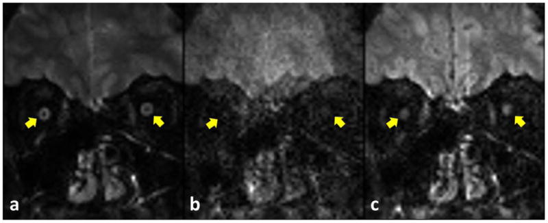
Multishot images (1.25×3 mm³) of non-DW (a) and 500 s/mm² (b,c) before (b) and after (c) motion-induced phase correction using 2-D navigator. Images without (b) and with (c) correction were reconstructed using the same NSA. The positions near subject's left and right optic nerves are marked as right and left yellow arrows in each figure, respectively.

Figure 2 and 3 compares the images obtained with the ssh- (Figs.2 and 3 a, b) and msh-DTI (Figs.2 and 3 c,d,e,f) images of the retrobulbar (Fig.2) and intraorbital (Fig.3) optic nerve for non-DW (Figs.2 and 3 a,c,e) and DW images at b=500 s/mm² (Figs.2 and 3 b,d,f) at 1.5 × 3 mm³ (Figs.2 and 3 a,b,c,d) and 1.25 × 3 mm³ (Figs.2 and 3 e,f) resolution, respectively. The size differences between optic nerve segments can be appreciated between different resolutions, and the conspicuity of the optic nerve is visibly greater in msh-DTI acquisitions than the ssh for both the b=500 s/mm² and the non-DW acquisitions. Also, little geometric distortion and blurring is appreciated in the msh DW (d,f) and non-DW (c,e) scans near the ocular muscles, and inferior brain tissue. Note that larger partial volume effects are seen in msh with 1.5 mm² vs. 1.25 mm², but geometric distortions are substantially smaller compared to single-shot counterparts.

Figure 2.

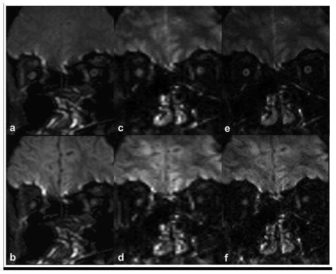
Comparison between ssh-DTI (a,b) and msh-DTI (c,d,e,f) images for retrobulbar optic nerve regions for non-DW (a,c,e) and DW (b,d,f) acquisitions. Acquisition voxels are 1.5×3 mm³ (a,b,c,d) and 1.25×3 mm³ (e,f) for ssh-DTI (a,b) and msh-DTI (c,d,e,f) acquisitions.

Figure 3.

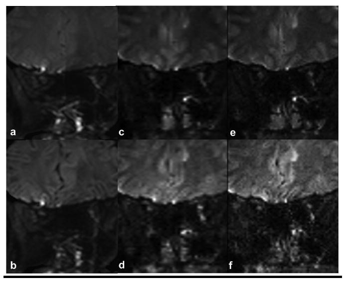
Comparison between ssh-DTI (a,b) and msh-DTI (c,d,e,f) images for intraorbital optic nerve regions for non-DW (a,c,e) and DW (b,d,f) acquisitions. Acquisition voxels are 1.5×3 mm³ (a,b,c,d) and 1.25×3 mm³ (e,f) for ssh-DTI (a,b) and msh-DTI (c,d,e,f) acquisitions.

Figure 4 presents DTI-derived maps (FA, MD, λ_⊥ and λ_⊥) from ssh- and msh-DTI (1.25 × 2 mm³) for both optic nerves. The ssh-DTI maps show significant geometric distortions and blurring in both nerves and signal asymmetry across nerves, whereas msh-DTI results show consistent bilateral nerve morphology and better contrast between the nerve and CSF than ssh counterparts. Both optic nerves are clearly delineated in all msh-DTI-derived maps, and showed lower (MD, λ_⊥ and λ_⊥) and higher (FA) values compared to surrounding CSF. In the msh FA map, the right optic nerve is a bright isolated spot, whereas the left optic nerve is less clear. In the ssh images, the right optic nerve is poorly resolved due to distortions, blurring and partial voluming with CSF, whereas the left optic nerve shows relatively clear FA and MD contrast and smaller image distortions. In general, ssh-DTI maps show poorer or similar contrasts in all DTI-derived maps compared with msh-DTI.

Figure 4.

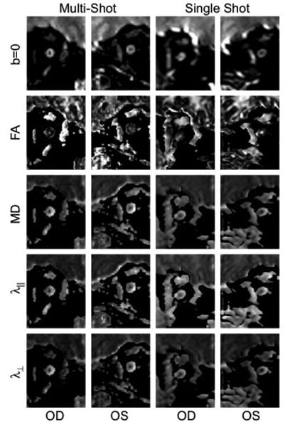
Maps of FA, MD, λ_∥ and λ_⊥ for the right and left optic nerves from each of representative msh-DTI (left two columns) and ssh-DTI (right two columns) acquisitions with 1.25×3 mm³ and 1.5×3 mm³ voxels for msh-DTI and ssh-DTI, respectively.

Quantitative DTI-derived Indices

Table 2 presents the descriptive (2a) and inferential (2b) statistics of the DTI-derived indices, across acquisition methods and voxel sizes for each eye. When comparing ssh-DTI and msh-DTI indices at 1.5 &times 3mm³ resolution, the average (over right and left) FA is lower, and the diffusivities higher in msh-DTI indices. However, for exclusively msh-DTI, at increasing resolution, the FA increases while the diffusivities decrease, potentially from reduced partial volume effects.

Table 2. Mean ± standard deviation of diffusion indices across methods for each (right and left) optic nerves.

	FA		†MD		†λ⊥		†λ⊥
Method	Right	Left	Right	Left	Right	Left	Right	Left
ssh 1.5 × 1.5 × 3mm3	0.52 ± 0.13	0.62 ± 0.15	1.09 ± 0.32	0.87 ± 0.37	1.74 ± 0.43	1.48 ± 0.45	0.76 ± 0.3	0.56 ± 0.35
msh 1.5 × 1.5 × 3mm3	0.54 ± 0.11	0.51 ± 0.11	1.35 ± 0.42	1.44 ± 0.39	2.17 ± 0.58	2.28 ± 0.54	0.94 ± 0.37	1.03 ± 0.36
msh 1.25 × 1.25 × 3mm3	0.63 ± 0.13	0.59 ± 0.13	1.14 ± 0.48	1.22 ± 0.47	1.99 ± 0.73	2.06 ± 0.7	0.73 ± 0.41	0.81 ± 0.42
msh 1.25 × 1.25 × 2mm3	0.64 ± 0.13	0.62 ± 0.15	1.11 ± 0.44	1.27 ± 0.44	1.96 ± 0.65	2.17 ± 0.64	0.69 ± 0.37	0.82 ± 0.4

^†μm²/ms scale

Since we studied only healthy volunteers, we do not expect an appreciable asymmetry between optic nerves. However, for ssh acquisition, all DTI-derived indices are significantly different between left and right optic nerves (weighted t-test, p-values: FA<0.001, MD=0.002, λ_⊥=0.003, λ_⊥=0.004). For msh-DTI, small differences were noted between right and left optic nerves, even over different voxel sizes (p-values from 0.3 to 0.4 for 1.5 × 1.5 × 3 mm³, 0.07 to 0.6 for 1.25 × 1.25 × 3 mm³ and 0.02 to 0.2 for 1.25 × 1.25 × 2 mm³) with the only significant difference being MD at 1.25 × 1.25 × 2 mm³ (p=0.02).

We also compared the impact of resolution on the mean values of the msh DTI-derived indices. All DTI-derived indices are statistically different (at α = 0.05) between in-plane resolutions of 1.5 mm² and 1.25 mm² (p-values: FA < 0.001, MD < 0.001, λ_⊥< 0.001, λ_⊥ = 0.03), yet no significant differences were observed between msh-DTI acquisitions with 2 and 3 mm slice thickness for in-plane resolution=1.25 mm. This suggests that higher in-plane resolution decreases the impact of partial volume with surrounding CSF regions more so than slice thickness.

We next compared ssh-DTI to msh-DTI acquisitions at matched resolutions in two ways. First, we examined the weighted means of each index over both eyes. At 1.5 × 1.5 × 3 mm³, all DTI-derived indices significantly depended on technique (between ssh- and msh p-values: FA = 0.02, MD < 0.001, λ_⊥< 0.001, λ_⊥ < 0.001). We hypothesize that this is likely due to blurring, geometric distortion and variation across eyes seen in the ssh method and indicates that the descriptive statistics may be dependent on optic nerve orientation in the ssh case (see Discussion). A source of error can arise from nested variance and the utilization of a weighted mean may overestimate the impact of technique. Therefore, we also compared resolution-matched ssh-DTI and msh-DTI-derived indices using the MAD statistical framework. Briefly, we report the MAD (mean absolute difference between the right and left optic nerves drawn from an empirically determined distribution), the 95% CI for MAD, and the δMAD%, which is the relative difference between the ssh-DTI and msh-DTI MAD value (note a negative value indicates improved MAD in the msh-DTI case compared to the ssh). Table 3 shows the MAD analysis, which, at the α = 0.05 level, there is no statistical evidence that the disparity between the right and left optic nerves is significant. One can loosely claim that there is no difference in the mean values of the two methods to draw an analogy to ANOVA. However, that the MAD is reduced in the msh-DTI acquisition compared to the ssh-DTI acquisition presents an improvement in the δMAD% of about 3% (λ_⊥) up to 17% (FA) indicating that across eyes, msh-DTI outperforms the ssh-DTI.

Table 3. MAD between left and right optic nerves at the initial time point. Also the 95% CI (MAD) and the relative improvement (−) or worsening (+) of msh-DTI vs. ssh-DTI techniques for each of the DTI-derived indices.

		FA			MD (μm2/ms)
Method	MAD	95%CI	δMAD%	MAD (×10−1)	95%CI (×10−1)	δMAD%
ssh 1.5×1.5×3mm3	0.18	(0.15, 0.2)	−16.7	4.2	(3.5, 5.1)	−14.3
msh 1.5×1.5×3mm3	0.15	(0.13, 0.17)		3.6	(3.1, 4.0)

		λ⊥ (μm2/ms)			λ⊥ (μm2/ms)
Method	MAD (×10−1)	95%CI (×10−1)	δMAD%	MAD (×10−1)	95%CI (×10−1)	δMAD%
ssh 1.5×1.5×3m×3	5.4	(4.0, 6.6)	−13.0	3.9	(3.3, 4.4)	−2.6
msh 1.5×1.5×3mm3	4.7	(4.1, 5.2)		3.8	(3.2, 4.3)

Reproducibility

In addition to comparison of indices across resolutions, we consider the reproducibility of the technique over time and an estimate of the robustness to voxel placement. The latter is critical for understanding the impact that such a technique can have in the clinic when manual ROIs are drawn for every patient/time. We compared each method across two time points using Bland-Altman and Wilcoxon signed-rank tests for each acquisition and resolution. Details of these analyses can be found in Table 4. The absolute mean differences (|D̄₁₂|) of the indices between two visits (Scan 1 and 2 in Table 4) are all small, and, additionally, Wilcoxon signed-rank tests demonstrate no statistically significant differences in the index mean values across visits for all acquisitions. Comparing msh-DTI 1.25 × 2 mm³ with the ssh-DTI 1.5 × 3 mm³ acquisitions, each msh DTI-derived index has a lower D_BA compared to ssh-DTI. For each 1.25 × 2 mm³ the D_BA remains below 10% indicating a high degree of reliability. However, the msh-DTI acquisition with 1.5 × 3mm³ and 1.25 × 3 mm³ voxels show larger D_BA than ssh-DTI for FA (1.5 × 3mm³) and λ_⊥ (1.25 × 3mm³).

Table 4. Reproducibility results from Bland-Altman and Wilcoxon signed-rank test.

		voxel (mm)	mean ± std†		D̄12†	95% CI (D) †	LOA†	p-value‡	DBA (%)
			Scan 1	Scan 2
FA	ssh	1.5 × 1.5 × 3	0.52 ± 0.08	0.54 ± 0.07	-0.03	(−0.17, 0.12)	(−0.26, 0.20)	0.81	5.49
	msh	1.5 × 1.5 × 3	0.54 ± 0.07	0.47 ± 0.13	0.08	(−0.03, 0.19)	(−0.10, 0.26)	0.13	15.65
		1.25 × 1.25 × 3	0.59 ± 0.09	0.61 ± 0.05	-0.02	(−0.13, 0.08)	(−0.22, 0.18)	0.69	3.55
		1.25 × 1.25 × 2	0.62 ± 0.05	0.62 ± 0.05	0.01	(−0.08, 0.06)	(−0.14, 0.12)	0.81	1.21
MD	ssh	1.5 × 1.5 × 3	1.20 ± 0.26	1.0 ± 0.23	0.21	(−0.25, 0.66)	(−0.52, 0.94)	0.31	18.94
	msh	1.5 × 1.5 × 3	1.53 ±0.43	1.51 ± 0.37	0.02	(−0.38, 0.42)	(−0.62, 0.66)	0.88	1.41
		1.25 × 1.25 × 3	1.53 ± 0.42	1.26 ± 0.31	0.27	(−0.07, 0.61)	(−0.39, 0.93)	0.09	19.15
		1.25 × 1.25 × 2	1.31 ± 0.32	1.41 ± 0.34	-0.09	(−0.39, 0.20)	(−0.67, 0.48)	0.44	6.98
λ⊥	ssh	1.5 × 1.5 × 3	1.9 ± 0.41	1.60 ±0.32	0.31	(−0.45, 1.08)	(−0.92, 1.54)	0.44	17.87
	msh	1.5 × 1.5 × 3	2.51 ± 0.59	2.38 ± 0.61	0.12	(−0.51, 0.75)	(−0.89, 1.14)	0.63	5.03
		1.25 × 1.25 × 3	2.5 ± 0.55	2.15 ± 0.52	0.36	(−0.23, 0.94)	(−0.77, 1.49)	0.16	15.47
		1.25 × 1.25 × 2	2.23 ± 0.42	2.39 ± 0.6	-0.16	(−0.67, 0.36)	(−1.15, 0.84)	0.56	6.77
λ⊥	ssh	1.5 × 1.5 × 3	0.85 ± 0.22	0.7 ± 0.19	0.16	(−0.17, 0.49)	(−0.37, 0.69)	0.44	20.15
	msh	1.5 × 1.5 × 3	1.05 ± 0.36	1.07 ± 0.28	-0.03	(−0.51, 0.75)	(−0.50, 0.44)	0.88	2.71
		1.25 × 1.25 × 3	1.04 ± 0.38	0.82 ± 0.21	0.21	(−0.08, 0.51)	(−0.35, 0.78)	0.06	22.91
		1.25 × 1.25 × 2	0.85 ± 0.27	0.92 ± 0.22	-0.06	(−0.27, 0.14)	(−0.45, 0.32)	0.56	7.25

^†μm²/ms scale

^‡Wilcoxon signed-rank test

When comparing msh- and ssh- at matched resolution, the msh D_BA is lower for all diffusivities (not FA) coarsely indicating a smaller variability across acquisitions when using msh-DTI acquisitions. However, as with cross-sectional analyses, we may have overestimated the differences due to nested variance and thus assessed MAD analyses between time points for matched resolutions as described in the methods. In this case, the MAD is the difference between time 1 and time 2 for either optic nerve as they are assumed to be interchangeable (c.f. methods). In Table 5, all derived indices except λ_⊥, shows msh- MAD is lower than ssh-, but there is no statistical evidence at the α = 0.05 level that the reproducibility is significantly different between the two techniques. It should be pointed out, however, that the δMAD% is improved (negative δMAD%) in the msh-DTI case compared to the ssh-DTI case (∼30-40% decrease) for indices except msh λ_⊥ which performs approximately 10% poorer than the ssh-DTI. To summarize the data presented in Table 2 and Table 4, figure 5 presents boxplot comparing diffusion indices for right (R) and left (L) optic nerve asymmetry (Fig 5a) and test (v1) and retest (v2) reproducibility (Fig5b) for each diffusion index. It should be pointed out, that the box-plot demonstrates the median, intra-quartile range and outliers of each index rather than the weighted mean over slices as is presented in the tables. It is important to present the box-plot data in this manner to demonstrate the impact of comparing the weighted contributions of each person on the summary statistics.

Table 5. MAD between initial and follow up exam. Data selected from a distribution that contains only the right eye, but assumed to be exchangeable and homogeneous. Also the 95% CI (MAD) and the relative improvement (−) or worsening (+) of msh-DTI compared to ssh-DTI techniques for each of the DTI-derived indices.

		FA			MD (μm2/ms)
Method	MAD	95%CI	δMAD%	MAD (×10−1)	95%CI (×10−1)	δMAD%
ssh 1.5×1.5×3mm3	0.21	(0.15, 0.32)	-28.6	5.1	(2.8, 8.1)	−31.4
msh 1.5×1.5×3mm3	0.15	(0.11,0.17)		3.5	(2.0, 5.1)

		λ⊥ (μm2/ms)			λ⊥ (μm2/ms)?
Method	MAD (×10−1)	95%CI (×10−1)	δMAD%	MAD (×10−1)	95%CI (×10-1)	δMAD%
ssh 1.5×1.5×3mm3	5.1	(3.1, 6.9)	9.8	5.3	(3.0, 9.0)	−37.7
msh 1.5×1.5×3mm3	5.6	(3.9, 6.9)		3.3	(3.2, 4.6)

Figure 5.

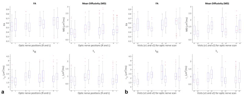
Boxplot comparing diffusion indices for right (R) and left (L) optic nerve asymmetry (a) and test (v1) and retest (v2) reproducibility (b) for each of diffusion indices.

Discussion and Conclusions

We implemented a DW msh EPI with SENSE and 2-D navigated motion correction to study the human optic nerve in vivo. DTI-derived indices of FA, MD, λ_∥ and λ_⊥ were acquired and compared between conventional ssh-DTI and msh-DTI approaches. When visually compared at the same resolution, msh-DTI provides much less geometric distortions and blurring effects compared to conventional ssh-EPI approaches. The descriptive statistics indicate that DTI-derived indices are consistent with previous reports on healthy volunteers. For example, Chabert et al.(8) reported FA values ranging from 0.39 to 0.56, MD: 0.8 to 1.3 μm²/ms (MD) and Wheeler-Kingshott et al.(20) presented FA values of 0.57 to 0.64 and MD: 1.17 to 1.27 μm²/ms, where our study shows FA ranges from 0.51 to 0.64 and MD from 0.87 to 1.44 μm²/ms (see Fig. 6 in Techavipoo et al. (17) for values from other studies). Interestingly, asymmetry between left and right optic nerves are not significant in Techavipoo et al. (17) even before the correction of susceptibility-induced distortions using field mapping, though the values from the right optic nerve tended to be lower than the left. This can be attributed to ocular fixation during scanning, larger number (32 vs. 15) of diffusion-encoding directions and CSF suppression. Although we chose less constrained imaging conditions for our subjects in anticipation of clinical implementation and comparison across techniques, assessing the impact of adapting such techniques for msh- and ssh-techniques is necessary. The main benefit, however, is the ability to improve optic nerve DTI by reducing EPI artifacts for optic nerve DW imaging at higher resolution. Because the msh-DTI methods are time limited, not the echo-train length, it is conceivable to extend this approach to 1 mm or less in-plane resolution with little impact from EPI-related artifacts.

All DTI- derived indices were significantly asymmetric in ssh-DTI scans, but not in the msh-DTI comparisons across eyes. This suggests that msh-DTI acquisitions may be more robust than ssh-DTI for bilateral comparisons of optic nerves, and more reliable for unilateral acquisitions. Additionally, we showed that the test-retest reproducibility was not significantly different across time points for all acquisitions, which agrees with previous ssh-DTI literature. Although msh-DTI acquisitions resulted in generally lower D_BA than ssh-DTI acquisitions, we observed minor exceptions in msh-DTI. This is not surprising due to the greater sensitivity of msh-DTI methods: i.e. a blurry image is often more reproducible than a sharp image due to the sensitivity to borders and ROI placement. It is a bit unfair to compare reproducibility of ssh-DTI to msh-DTI at different resolutions due to the impact of SNR, CNR, and general blurring in ssh-DTI acquisitions. When considering matched resolution, there is approximately a 30% reduction in the scan-to-scan variability in the msh-DTI compared to the ssh-DTI. Visually, msh-DTI acquisitions showed superior image quality and optic nerve conspicuity when compared to ssh-DTI. It should be noted that low CNR and poor resolution may lead to greater scan-rescan reliability and future statistical studies could derive statistical models that penalize scans with poor resolution and/or CNR.

We chose to compare scans with an equal scan time unit rather than adjusting angular resolution of diffusion gradients which can adversely impact the fidelity of the derived indices (49). Therefore, ssh-DTI scans were acquired with more signal acquisitions (N_avg) than the msh-DTI scans to match the scan time, e.g., N_avg = 10 (1.5 × 3 mm³) for ssh-DTI vs. N_avg = 8 (1.5 × 3 mm³) and N_avg = 5 (1.25 mm²) for msh-DTI. Although increasing N_avg can increase SNR, EPI-related artifacts cannot be reduced unless the EPI echo-train length is reduced. With the developed acquisition and reconstruction methods, DTI scans were performed with higher phase-encoding bandwidth (ssh=34 Hz vs. msh=91 Hz) and shorter echo-trains (52 in ref. (12) and 48 in ref. (21)) than conventional ssh-DTI, and, hence, clearer optic nerve images can be appreciated and image distortion, blurring and eddy-current effects are significantly mitigated.

The msh-DTI imaging sequence only acquires a segment of k-space for each excitation, and k-space is filled over multiple TR periods. When the diffusion gradients are on, gross subject or physiological motions can generate additional phase in the DW signal, proportional to the magnitude of motion or the gradient. The phase variation depends on the orientations of the axis of rotation and the applied diffusion gradient. Therefore, more than a 1-D navigator is required for correction of motion-induced phase errors typical in msh-DTI acquisitions. In this study a 2-D navigator-echo was acquired using additional EPI readout for more accurate corrections of in-plane phase variations. The use of 2-D navigators for phase correction has been effective even for the correction of nonlinear motion-induced phases, e.g., nonlinear brain motion by cardiac pulsation (36).

A major difficulty in optic nerve imaging is rapid, random eye motion which affects the position/orientation of the optic nerve. Although ssh-DTI can acquire an image within a fraction of second, effects between acquisitions for different diffusion gradient orientations and averaging (50). Although the optic nerve is visually more conspicuous in msh non-DW and DW images than in ssh-DTI images (Figs. 2 and 3), larger, uncompensated motion effects hamper msh-DTI more so than ssh-DTI. Previous literature shows that averaging a large number of acquisitions (> 40) can reduce the effect of motion and is effective for localization of the optic nerve when the ZOOM technique is used (10,19,20). In our current study, five to eight acquisitions were averaged for msh-DTI scans (10 for ssh-DTI) to cover 12 slices (36 mm with 3 mm slice thickness) with 15 diffusion-weighting gradients. These scan parameters provided high-quality msh non-DW and DW images within clinically acceptable scan time (< 8 min) with reduced Nyquist violation in msh scans (≥ 4 acquisitions for averaging (51)), extended coverage along the optic nerve (36 mm (42)) and reduced variation in DTI-derived indices (>> 6 directions (52)). Although the scan time constraint in the presence of other scan parameters allowed relatively short msh TRs (∼ 2 s), there was no significant visual impact on msh non-DW and DW images (Figs. 1, 2 and 3) and derived indices (Fig. 4). Note that the left optic nerve appears less clear than the right in msh-DTI FA map. This may be due to eye motion and/or a partial volume effect from postero-medially running optic nerve geometry, because the effect is manifested in the left optic nerve diffusivity maps where the nasal-lateral aspect of the left optic nerve region appears darker than medial aspect.

It should be noted that this study was designed to image both optic nerves simultaneously for comparisons with conventional acquisition methodology. The optic nerve does not follow a straight path, and in most subjects the intraorbital optic nerves courses oblique to the imaging plane. In addition, uncontrolled eye movement without ocular fixation and uncompensated CSF signal may affect DTI measurements as well as major white matter tracts (53,54) depending on the amount of eye motion, nerve angulations and slice thicknesses. The results may suggest that increased through-plane partial volume effects are more detrimental in tissue-CSF than tissue-tissue boundaries. One potential way to mitigate through-plane partial volume would be to study each optic nerve individually and set the imaging planes as coronal (or sagittal/axial) to each nerve, or perform CSF suppression. Also notable is the reduction of water signal intensity by RF pulses (SPIR or SPAIR) or gradient inversion. This unwanted suppression of water signals, especially, can cause extra signal loss resulting in errors in quantitative DTI analysis. Future studies could include a study of appropriate tissue and CSF suppression techniques for msh-DTI.

The cohort tested were all healthy volunteers. The next step is to evaluate if msh-DTI can provide a viable alternative to ssh-DTI for studies of optic nerve pathologies. We suspect higher resolution would be necessary in such cases which is feasible with msh-DTI. Lastly, purpose designed and higher channel receive coils could improve upon the optic nerve methodology presented here with a conventional 8-channel SENSE head coil.

List of Symbols

i

Italic i

j

Italic j

k

Italic k

R

Italic R

References

- 1.Balcer LJ. Clinical practice. Optic neuritis. New Engl J Med. 2006;354:1273–1280. doi: 10.1056/NEJMcp053247. [DOI] [PubMed] [Google Scholar]
- 2.Hickman SJ, Miszkiel KA, Plant GT, Miller DH. The optic nerve sheath on MRI in acute optic neuritis. Neuroradiology. 2005;47:51–55. doi: 10.1007/s00234-004-1308-x. [DOI] [PubMed] [Google Scholar]
- 3.Kupersmith MJ, Alban T, Zeiffer B, Lefton D. Contrast-enhanced MRI in acute optic neuritis: relationship to visual performance. Brain. 2002;125:812–822. doi: 10.1093/brain/awf087. [DOI] [PubMed] [Google Scholar]
- 4.Boorstein JM, Moonis G, Boorstein SM, Patel YP, Culler AS. Optic neuritis: imaging with magnetization transfer. AJR American journal of roentgenology. 1997;169:1709–1712. doi: 10.2214/ajr.169.6.9393194. [DOI] [PubMed] [Google Scholar]
- 5.Dousset V, Grossman RI, Ramer KN, Schnall MD, Young LH, Gonzalez-Scarano F, Lavi E, Cohen JA. Experimental allergic encephalomyelitis and multiple sclerosis: lesion characterization with magnetization transfer imaging. Radiology. 1992;182:483–491. doi: 10.1148/radiology.182.2.1732968. [DOI] [PubMed] [Google Scholar]
- 6.Hickman SJ, Toosy AT, Jones SJ, Altmann DR, Miszkiel KA, MacManus DG, Barker GJ, Plant GT, Thompson AJ, Miller DH. Serial magnetization transfer imaging in acute optic neuritis. Brain. 2004;127:692–700. doi: 10.1093/brain/awh076. [DOI] [PubMed] [Google Scholar]
- 7.Schmierer K, Scaravilli F, Altmann DR, Barker GJ, Miller DH. Magnetization transfer ratio and myelin in postmortem multiple sclerosis brain. Annals of Neurology. 2004;56:407–415. doi: 10.1002/ana.20202. [DOI] [PubMed] [Google Scholar]
- 8.Chabert S, Molko N, Cointepas Y, Le Roux P, Le Bihan D. Diffusion tensor imaging of the human optic nerve using a non-CPMG fast spin echo sequence. J Magn Reson Imaging. 2005;22:307–310. doi: 10.1002/jmri.20383. [DOI] [PubMed] [Google Scholar]
- 9.Dowell NG, Jenkins TM, Ciccarelli O, Miller DH, Wheeler-Kingshott CA. Contiguous-slice zonally oblique multislice (CO-ZOOM) diffusion tensor imaging: examples of in vivo spinal cord and optic nerve applications. J Magn Reson Imaging. 2009;29:454–460. doi: 10.1002/jmri.21656. [DOI] [PubMed] [Google Scholar]
- 10.Hickman SJ, Wheeler-Kingshott CA, Jones SJ, Miszkiel KA, Barker GJ, Plant GT, Miller DH. Optic nerve diffusion measurement from diffusion-weighted imaging in optic neuritis. AJNR Am J Neuroradiol. 2005;26:951–956. [PMC free article] [PubMed] [Google Scholar]
- 11.Iwasawa T, Matoba H, Ogi A, Kurihara H, Saito K, Yoshida T, Matsubara S, Nozaki A. Diffusion-weighted imaging of the human optic nerve: a new approach to evaluate optic neuritis in multiple sclerosis. Magn Reson Med. 1997;38:484–491. doi: 10.1002/mrm.1910380317. [DOI] [PubMed] [Google Scholar]
- 12.Kim SE, Jeong EK, Kim TH, Hadley JR, Minagla E, Anderson J, Parker DL. In Vivo Diffusion Tensor Imaging of Human Optic Nerve Using 2D Interleaved Inner Volume Technique on 3T System. Proceedings of the 16th Annual Meeting of ISMRM; Toronto, Canada. 2008. p. 1815. [Google Scholar]
- 13.Naismith RT, Xu J, Snyder A, Benzinger T, Shimony J, Trinkaus K, Cross AH, Song SK. Axial Diffusivity in Acute and Isolated Optic Neuritis. Proceedings of the 16th Annual Meeting of ISMRM; Toronto, Canada. 2008. p. 3392. [Google Scholar]
- 14.Naismith RT, Xu J, Tutlam NT, Snyder A, Benzinger T, Shimony J, Shepherd J, Trinkaus K, Cross AH, Song SK. Disability in optic neuritis correlates with diffusion tensor-derived directional diffusivities. Neurology. 2009;72:589–594. doi: 10.1212/01.wnl.0000335766.22758.cd. [DOI] [PMC free article] [PubMed] [Google Scholar]
- 15.Smith SA, Williams ZR, Ratchford JN, Newsome SD, Farrell SK, Farrell JA, Gifford A, Miller NR, van Zijl PC, Calabresi PA, Reich DS. Diffusion tensor imaging of the optic nerve in multiple sclerosis: association with retinal damage and visual disability. AJNR American journal of neuroradiology. 2011;32:1662–1668. doi: 10.3174/ajnr.A2574. [DOI] [PMC free article] [PubMed] [Google Scholar]
- 16.Sun HH, Wang D, Zhang QJ, Bai ZL, He P. Magnetic resonance diffusion tensor imaging of optic nerve and optic radiation in healthy adults at 3T. International journal of ophthalmology. 2013;6:868–872. doi: 10.3980/j.issn.2222-3959.2013.06.22. [DOI] [PMC free article] [PubMed] [Google Scholar]
- 17.Techavipoo U, Okai AF, Lackey J, Shi J, Dresner MA, Leist TP, Lai S. Toward a practical protocol for human optic nerve DTI with EPI geometric distortion correction. J Magn Reson Imaging. 2009;30:699–707. doi: 10.1002/jmri.21836. [DOI] [PubMed] [Google Scholar]
- 18.van der Walt A, Kolbe SC, Wang YE, Klistorner A, Shuey N, Ahmadi G, Paine M, Marriott M, Mitchell P, Egan GF, Butzkueven H, Kilpatrick TJ. Optic nerve diffusion tensor imaging after acute optic neuritis predicts axonal and visual outcomes. PLoS One. 2013;8:e83825. doi: 10.1371/journal.pone.0083825. [DOI] [PMC free article] [PubMed] [Google Scholar]
- 19.Wheeler-Kingshott CA, Parker GJ, Symms MR, Hickman SJ, Tofts PS, Miller DH, Barker GJ. ADC mapping of the human optic nerve: increased resolution, coverage, and reliability with CSF-suppressed ZOOM-EPI. Magn Reson Med. 2002;47:24–31. doi: 10.1002/mrm.10016. [DOI] [PubMed] [Google Scholar]
- 20.Wheeler-Kingshott CA, Trip SA, Symms MR, Parker GJ, Barker GJ, Miller DH. In vivo diffusion tensor imaging of the human optic nerve: pilot study in normal controls. Magn Reson Med. 2006;56:446–451. doi: 10.1002/mrm.20964. [DOI] [PubMed] [Google Scholar]
- 21.Xu JG, Naismith RT, Trinkaus KM, Cross AH, Song SK. Towards Accurate In Vivo Diffusion Measurement in Human Optic Nerve. Proceedings of the 15th Annual Meeting of ISMRM; Berlin, Germany. 2007. p. 11. [Google Scholar]
- 22.Basser PJ, Mattiello J, LeBihan D. Estimation of the effective self-diffusion tensor from the NMR spin echo. J Magn Reson B. 1994;103:247–254. doi: 10.1006/jmrb.1994.1037. [DOI] [PubMed] [Google Scholar]
- 23.Moseley ME, Cohen Y, Kucharczyk J, Mintorovitch J, Asgari HS, Wendland MF, Tsuruda J, Norman D. Diffusion-weighted MR imaging of anisotropic water diffusion in cat central nervous system. Radiology. 1990;176:439–445. doi: 10.1148/radiology.176.2.2367658. [DOI] [PubMed] [Google Scholar]
- 24.Basser PJ, Pierpaoli C. Microstructural and physiological features of tissues elucidated by quantitative-diffusion-tensor MRI. Journal of magnetic resonance Series B. 1996;111:209–219. doi: 10.1006/jmrb.1996.0086. [DOI] [PubMed] [Google Scholar]
- 25.Le Bihan D, Breton E, Lallemand D, Grenier P, Cabanis E, Laval-Jeantet M. MR Imaging of Intravoxel Incoherent Motions: Application to Diffusion and Perfusion in Neurologic Disorders. Radiology. 1986;161:401–407. doi: 10.1148/radiology.161.2.3763909. [DOI] [PubMed] [Google Scholar]
- 26.Trip SA, Wheeler-Kingshott C, Jones SJ, Li WY, Barker GJ, Thompson AJ, Plant GT, Miller DH. Optic nerve diffusion tensor imaging in optic neuritis. Neuroimage. 2006;30:498–505. doi: 10.1016/j.neuroimage.2005.09.024. [DOI] [PubMed] [Google Scholar]
- 27.Frohman EM, Fujimoto JG, Frohman TC, Calabresi PA, Cutter G, Balcer LJ. Optical coherence tomography: a window into the mechanisms of multiple sclerosis. Nat Clin Pract Neurol. 2008;4:664–675. doi: 10.1038/ncpneuro0950. [DOI] [PMC free article] [PubMed] [Google Scholar]
- 28.Turner R, Le Bihan D. Single-shot diffusion imaging at 2.0 tesla. J Magn Reson. 1990;86:445–452. [Google Scholar]
- 29.Pruessmann KP, Weiger M, Scheidegger MB, Boesiger P. SENSE: sensitivity encoding for fast MRI. Magn Reson Med. 1999;42:952–962. [PubMed] [Google Scholar]
- 30.Anderson AW, Gore JC. Analysis and correction of motion artifacts in diffusion weighted imaging. Magn Reson Med. 1994;32:379–387. doi: 10.1002/mrm.1910320313. [DOI] [PubMed] [Google Scholar]
- 31.Ordidge RJ, Helpern JA, Qing ZX, Knight RA, Nagesh V. Correction of motional artifacts in diffusion-weighted MR images using navigator echoes. Magn Reson Imaging. 1994;12:455–460. doi: 10.1016/0730-725x(94)92539-9. [DOI] [PubMed] [Google Scholar]
- 32.Atkinson D, Counsell S, Hajnal JV, Batchelor PG, Hill DL, Larkman DJ. Nonlinear phase correction of navigated multi-coil diffusion images. Magn Reson Med. 2006;56:1135–1139. doi: 10.1002/mrm.21046. [DOI] [PubMed] [Google Scholar]
- 33.Butts K, Pauly J, de Crespigny A, Moseley M. Isotropic diffusion-weighted and spiral-navigated interleaved EPI for routine imaging of acute stroke. Magn Reson Med. 1997;38:741–749. doi: 10.1002/mrm.1910380510. [DOI] [PubMed] [Google Scholar]
- 34.Liu C, Bammer R, Kim DH, Moseley ME. Self-navigated interleaved spiral (SNAILS): application to high-resolution diffusion tensor imaging. Magn Reson Med. 2004;52:1388–1396. doi: 10.1002/mrm.20288. [DOI] [PubMed] [Google Scholar]
- 35.Liu C, Moseley ME, Bammer R. Simultaneous phase correction and SENSE reconstruction for navigated multi-shot DWI with non-cartesian k-space sampling. Magn Reson Med. 2005;54:1412–1422. doi: 10.1002/mrm.20706. [DOI] [PubMed] [Google Scholar]
- 36.Miller KL, Pauly JM. Nonlinear phase correction for navigated diffusion imaging. Magn Reson Med. 2003;50:343–353. doi: 10.1002/mrm.10531. [DOI] [PubMed] [Google Scholar]
- 37.Pipe JG, Farthing VG, Forbes KP. Multishot diffusion-weighted FSE using PROPELLER MRI. Magn Reson Med. 2002;47:42–52. doi: 10.1002/mrm.10014. [DOI] [PubMed] [Google Scholar]
- 38.Porter DA, Heidemann RM. High resolution diffusion-weighted imaging using readout-segmented echo-planar imaging, parallel imaging and a two-dimensional navigator-based reacquisition. Magn Reson Med. 2009;62:468–475. doi: 10.1002/mrm.22024. [DOI] [PubMed] [Google Scholar]
- 39.Frank LR, Jung Y, Inati S, Tyszka JM, Wong EC. High efficiency, low distortion 3D diffusion tensor imaging with variable density spiral fast spin echoes (3D DW VDS RARE) Neuroimage. 2010;49:1510–1523. doi: 10.1016/j.neuroimage.2009.09.010. [DOI] [PMC free article] [PubMed] [Google Scholar]
- 40.Van AT, Hernando D, Sutton BP. Motion-induced phase error estimation and correction in 3D diffusion tensor imaging. IEEE transactions on medical imaging. 2011;30:1933–1940. doi: 10.1109/TMI.2011.2158654. [DOI] [PubMed] [Google Scholar]
- 41.Jeong HK, Gore JC, Anderson AW. High-resolution human diffusion tensor imaging using 2-D navigated multishot SENSE EPI at 7 T. Magn Reson Med. 2013;69:793–802. doi: 10.1002/mrm.24320. [DOI] [PMC free article] [PubMed] [Google Scholar]
- 42.Barker GJ. Diffusion-weighted imaging of the spinal cord and optic nerve. J Neurol Sci. 2001;186(Suppl 1):S45–49. doi: 10.1016/s0022-510x(01)00490-7. [DOI] [PubMed] [Google Scholar]
- 43.Butts K, Riederer SJ, Ehman RL, Thompson RM, Jack CR. Interleaved echo planar imaging on a standard MRI system. Magn Reson Med. 1994;31:67–72. doi: 10.1002/mrm.1910310111. [DOI] [PubMed] [Google Scholar]
- 44.Feinberg DA, Oshio K. Phase errors in multi-shot echo planar imaging. Magn Reson Med. 1994;32:535–539. doi: 10.1002/mrm.1910320418. [DOI] [PubMed] [Google Scholar]
- 45.Basser PJ. Inferring microstructural features and the physiological state of tissues from diffusion-weighted images. NMR in Biomedicine. 1995;8:333–344. doi: 10.1002/nbm.1940080707. [DOI] [PubMed] [Google Scholar]
- 46.McAuliffe M, L E, McGarry D, Gandler W, Csaky K, Trus B. Medical image processing, analysis and visualization in clinical research. Proceedings of the 14th IEEE symposium on computer-based medical systems (CBMS 2001); 2001. pp. 381–6. [Google Scholar]
- 47.Bland JM, Kerry SM. Statistics notes. Weighted comparison of means Bmj. 1998;316:129. doi: 10.1136/bmj.316.7125.129. [DOI] [PMC free article] [PubMed] [Google Scholar]
- 48.Bland JM, Altman DG. Measuring agreement in method comparison studies. Stat Methods Med Res. 1999;8:135–160. doi: 10.1177/096228029900800204. [DOI] [PubMed] [Google Scholar]
- 49.Landman BA, Farrell JA, Jones CK, Smith SA, Prince JL, Mori S. Effects of diffusion weighting schemes on the reproducibility of DTI-derived fractional anisotropy, mean diffusivity, and principal eigenvector measurements at 1.5T. Neuroimage. 2007;36:1123–1138. doi: 10.1016/j.neuroimage.2007.02.056. [DOI] [PMC free article] [PubMed] [Google Scholar]
- 50.Storey P, Frigo FJ, Hinks RS, Mock BJ, Collick BD, Baker N, Marmurek J, Graham SJ. Partial k-space reconstruction in single-shot diffusion-weighted echo-planar imaging. Magn Reson Med. 2007;57:614–619. doi: 10.1002/mrm.21132. [DOI] [PubMed] [Google Scholar]
- 51.Atkinson D, Porter DA, Hill DL, Calamante F, Connelly A. Sampling and reconstruction effects due to motion in diffusion-weighted interleaved echo planar imaging. Magn Reson Med. 2000;44:101–109. doi: 10.1002/1522-2594(200007)44:1<101::aid-mrm15>3.0.co;2-s. [DOI] [PubMed] [Google Scholar]
- 52.Jones DK. The effect of gradient sampling schemes on measures derived from diffusion tensor MRI: a Monte Carlo study. Magn Reson Med. 2004;51:807–815. doi: 10.1002/mrm.20033. [DOI] [PubMed] [Google Scholar]
- 53.Bhagat YA, Beaulieu C. Diffusion anisotropy in subcortical white matter and cortical gray matter: changes with aging and the role of CSF-suppression. J Magn Reson Imaging. 2004;20:216–227. doi: 10.1002/jmri.20102. [DOI] [PubMed] [Google Scholar]
- 54.Papadakis NG, Martin KM, Mustafa MH, Wilkinson ID, Griffiths PD, Huang CL, Woodruff PW. Study of the effect of CSF suppression on white matter diffusion anisotropy mapping of healthy human brain. Magn Reson Med. 2002;48:394–398. doi: 10.1002/mrm.10204. [DOI] [PubMed] [Google Scholar]