Tree of Life Reveals Clock-Like Speciation and Diversification

Abstract

Genomic data are rapidly resolving the tree of living species calibrated to time, the timetree of life, which will provide a framework for research in diverse fields of science. Previous analyses of taxonomically restricted timetrees have found a decline in the rate of diversification in many groups of organisms, often attributed to ecological interactions among species. Here, we have synthesized a global timetree of life from 2,274 studies representing 50,632 species and examined the pattern and rate of diversification as well as the timing of speciation. We found that species diversity has been mostly expanding overall and in many smaller groups of species, and that the rate of diversification in eukaryotes has been mostly constant. We also identified, and avoided, potential biases that may have influenced previous analyses of diversification including low levels of taxon sampling, small clade size, and the inclusion of stem branches in clade analyses. We found consistency in time-to-speciation among plants and animals, ∼2 My, as measured by intervals of crown and stem species times. Together, this clock-like change at different levels suggests that speciation and diversification are processes dominated by random events and that adaptive change is largely a separate process.

Introduction

The evolutionary timetree of life (TTOL) is needed for understanding and exploring the origin and diversity of life (Hedges and Kumar 2009; Nei 2013). For this reason, scientists have been leveraging the genomics revolution and major statistical advances in molecular dating techniques to generate divergence times between populations and species. Collectively, tens of thousands of species have been timed, and new divergence time estimates are appearing in hundreds of publications each year (supplementary fig. S1, Supplementary Material online). A global synthesis of these results will allow direct comparison of the TTOL with the fossil record and Earth history and provide new opportunities for discovery of patterns and processes that operated in the past. The TTOL is also essential for studying the multidimensional nature of biodiversity and predicting how anthropogenic changes in our environment will impact the distribution and composition of biodiversity in the future (Hoffmann et al. 2010). A robust TTOL will provide a framework for research in diverse fields of science and medicine and a stimulus for science education. Data now exist for building a synthetic species-level TTOL of substantial size from the growing knowledge (supplementary fig. S1, Supplementary Material online).

There are challenges in synthesizing a global TTOL. The most common approach for constructing a large timetree using a sequence alignment or super alignment is possible (Smith and O'Meara 2012; Tamura et al. 2012), but not generally practical because of data matrix sparseness. For example, genes appropriate for closely related species are unalignable at higher levels, and those appropriate for higher levels are too conserved for resolving relationships of species. Disproportionate attention to some species, such as model organisms and groups of general interest (e.g., mammals and birds), also results in an uneven distribution of knowledge. In addition, computational limits are reached for Bayesian timing methods involving more than a few hundred species (Battistuzzi et al. 2011; Jetz et al. 2012).

Here, we have taken an approach to build a global TTOL by means of a data-driven synthesis of published timetrees into a large hierarchy. We have synthesized timetrees and related information in 2,274 molecular studies, which we collected and curated in a knowledgebase (Hedges et al. 2006) (supplementary Materials and Methods, Supplementary Material online). We mapped timetrees and divergence data from those studies on a robust and conservative guidetree based on community consensus (National Center for Biotechnology Information 2013) and used those times to resolve polytomies and derive nodal times in the TTOL (supplementary fig. S2, Supplementary Material online). We present this synthesis here, for use by the community, and explore how it bears on evolutionary hypotheses and mechanisms of speciation and diversification.

Results

A Global Timetree of Species

Our TTOL contains 50,632 species (fig. 1). Nearly all (∼99.5%) of the 1.9 million described species of living organisms are eukaryotes (Costello et al. 2013), and the proportion is similar (99.7%) in our TTOL (fig. 1). The naturally unbalanced shape of the TTOL, for example, with more eukaryote than prokaryote species, allowed us to present it in a unique spiral format to accommodate its large size. A “timeline” can be envisioned for each species in the TTOL, based on its sequence of branching events back in time to the origin of life. For example, a timeline from humans (fig. 2) captures evolutionary events that have received the most queries (74%) by users of the TimeTree knowledgebase (Hedges et al. 2006) (supplementary Materials and Methods, Supplementary Material online).

Fig. 1.

(2 columns) A timetree of 50,632 species synthesized from times of divergence published in 2,274 studies. Evolutionary history is compressed into a narrow strip and then arranged in a spiral with one end in the middle and the other on the outside. Therefore, time progresses across the width of the strip at all places, rather than along the spiral. Time is shown in billions of years on a log scale and indicated throughout by bands of gray. Major taxonomic groups are labeled and the different color ranges correspond to the main taxonomic divisions of our tree.

Fig. 2.

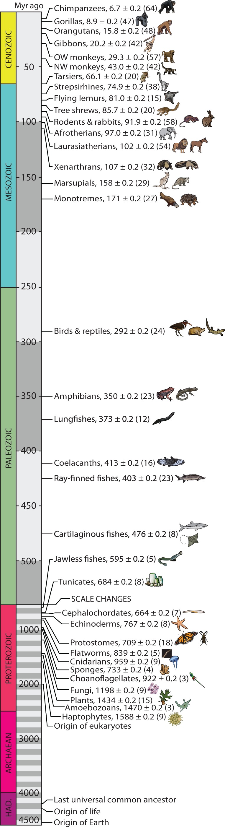
(1 column) A timeline from the perspective of humans, showing divergences with other groups of organisms. In each case, mean ± standard error (among studies) is shown, with number of studies in parentheses. Also shown are the times for the origin of life, eukaryotes, and last universal common ancestor (Hedges and Kumar 2009).

Linnaean taxonomic ranks exhibit temporal inconsistencies (fig. 3) as has been suggested in smaller surveys (Hedges and Kumar 2009; Avise and Liu 2011). For example, a class (higher rank) of angiosperm averages younger than an order (lower rank) of fungus, and an order of animal averages younger than a genus (low rank) of basidiomycete fungus. Ranks for prokaryotes are all older than the corresponding ranks of eukaryotes, with a genus of eubacteria averaging 715.7 ± 139.4 Ma compared with 12.6 ± 1.2 Ma for a genus of eukaryotes (fig. 3 and supplementary Materials and Methods, Supplementary Material online). These inconsistencies will cause difficulties in any scientific study comparing different types of organisms, where Linnaean rank is assumed to have a temporal equivalence.

Fig. 3.

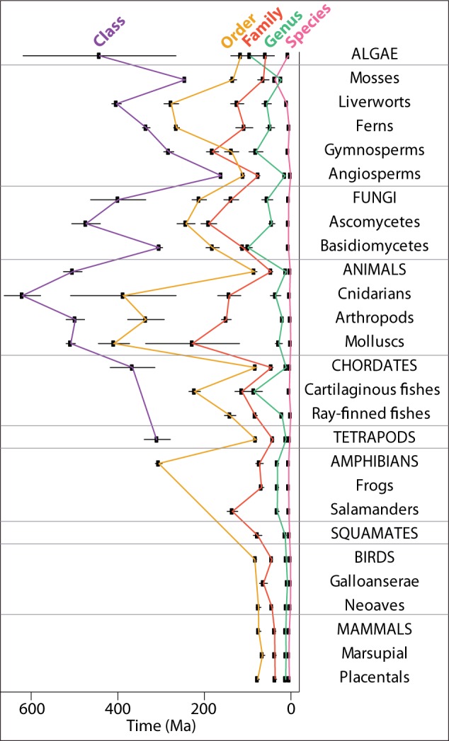
(1 column) Temporal relationships of Linnaean ranks of eukaryotes, showing mode and 95% confidence intervals. Prokaryotes are not shown because of large differences in scale (supplementary Materials and Methods, Supplementary Material online).

Diversification

The large TTOL afforded us the opportunity to examine patterns of lineage splitting across the diversity of eukaryotes (we omit prokaryotes in our TTOL analyses because they have an arbitrary species definition). Under models of “expansion,” diversity will continue to expand, either at an increasing diversification rate (hyper-expansion), the same rate (constant expansion), or decreasing rate (hypo-expansion). Saturation, on the other hand, refers to a drop in rate to zero as diversity reaches a plateau (equilibrium), possibly because of density-dependent biotic factors such as species interactions (Morlon 2014). Most recent analyses, but not all (Venditti et al. 2010; Jetz et al. 2012), have suggested that hypo-expansion is the predominant pattern in the tree of life, although there has been considerable debate as to the importance of timescales, biotic or abiotic factors, and potential biases in the analyses (Sepkoski 1984; Benton 2009; Morlon et al. 2010; Rabosky et al. 2012; Cornell 2013; Rabosky 2013).

Instead, we find that constant expansion and hyper-expansion are the dominant patterns of lineage diversification in the TTOL (fig. 4a). Our result was statistically significant irrespective of the method used, including diversification rate tests and simulations, a coalescent approach (not conducted for the TTOL), gamma tests, a clade age-size relationship (see Materials and Methods), and branch length distribution analysis (supplementary Materials and Methods, Supplementary Material online). The rate of diversification did not decrease over the history of eukaryotes (fig. 4). The same results were retrieved with another method (supplementary fig. S3, Supplementary Material online); we did not interpret the data before 1,000 Ma because only 37 lineages were present at this time, also explaining the large confidence intervals for this period. The observed diversification closely matched a simulated pure birth–death (BD) model, increasing slightly during the last 200 My (fig. 4a and b). The terminal drop in rate at ∼1 Ma is a normal characteristic of diversification plots (Etienne and Rosindell 2012) related to the taxonomic level selected for the study, in this case species. This “taxonomic bias” (rate drop) occurs at different times (Hedges and Kumar 2009) when genera, families, or other taxa are selected for study, because lower level clades (in this case, populations destined to become species) are omitted.

Fig. 4.

(1 column) Patterns of lineage diversification. (a) Cumulative lineages-through-time (LTT) curve for eukaryotes (50,455 sp.), in black, showing the number of lineages through time (unsmoothed, dashed; smoothed, solid) and variance (red, 500 replicates). (b) Same LTT curve (black line), but compared with a simulated constant-expansion LTT curve (λ (speciation rate) = 0.073 and μ (extinction rate) = 0.070) shown as ± 99% confidence intervals (red). (c) Diversification rate plot of same data showing only significant changes in rate as determined in maximum-likelihood tests; variance (red, 500 replicates) shown as ± 99% intervals.

The TTOL was partitioned into 58 diverse Linnaean clades (Actinopterygii, Afrotheria, Amazona, Ambystoma, Amphibia, Amphibolurinae, Amphisbaenia, angiosperms, Anguimorpha, Anolis, Anseriformes, birds, Boidae, Bolitoglossa, Canidae, Cetardiodactyla, Chamaeleo, Chondrichthyes, Ciconiiformes, Columbiformes, Cracidae, Cuculidae, Eleutherodactylus, Erinaceidae, Falco, Feliformia, Gymnophiona, gymnosperms, Hylarana, Hyloidea, Hynobius, Hyperolius, Iguanidae, Kinyongia, Lacertidae, Liolaemus, mammals, Megapodiidae, Metatheria, Moniliformopses, Musophagidae, Palaeognathae, Pelobatoidea, Perissodactyla, Phaeophyceae, Phasianidae, Plethodon, Podicipedidae, Primates, Ranoidea, Squamata, Suncus, Thamnophis, Tupaiidae, Ursidae, Varanus, Xenarthra, and Xenopus) for coalescence and gamma tests encompassing 44,958 total species (supplementary Materials and Methods, Supplementary Material online). The clades were chosen to represent taxonomic diversity and a range of clade size, clade age, and taxonomic sampling. Species sampling levels were high, with a median clade size of 66% of known species and 84% of the clades having 40% or more of known species. Among the 10 largest clades (Actinopterygii, Amphibia, angiosperms, birds, Ciconiiformes, Hyloidea, mammals, Moniliformopses, Ranoidea, Squamata), only one (angiosperms) showed hypo-expansion using the coalescent method, while the others were exclusively hyper-expanding. Low levels of sampling are known to bias toward hypo-expansion (Cusimano and Renner 2010; Moen and Morlon 2014), and the same clade (angiosperms) was also the most poorly sampled (5%). Also, there was no support in those clades for a decline in diversification rate using the gamma test. Although some methods can account for incomplete random sampling, the nonrandom sampling typically used by systematists (e.g., selecting for deeply branching lineages) is not accounted for by current methods and will bias results in favor of hypo-expansion (Cusimano and Renner 2010).

Focusing on the 48 smaller clades (e.g., genera and families) of tetrapods, we found that these likewise favored the expanding models (84% of clades showing significant results) rather than the saturation model (see Materials and Methods). Of those, most (87%) were either expanding or hyper-expanding, with only 13% hypo-expanding. Concerning the gamma test, 67% of these smaller clades did not show a decline in diversification rate through time, as was true for eukaryotes as a whole (fig. 4; gamma statistic = 136.4, P = 1). Hyper-expanding clades were significantly larger (fig. 5a; $\stackrel{�}{x},$831 vs. 91 species; P < 0.05) and older (fig. 5b; $\stackrel{�}{x}$, 104 vs. 57 Ma; P < 0.001) than other clades (see Materials and Methods). We also found that TTOL branch-length distribution fits an exponential distribution significantly better than other models (see Materials and Methods), agreeing with an earlier study (Venditti et al. 2010) using a small data set and approach.

Fig. 5.

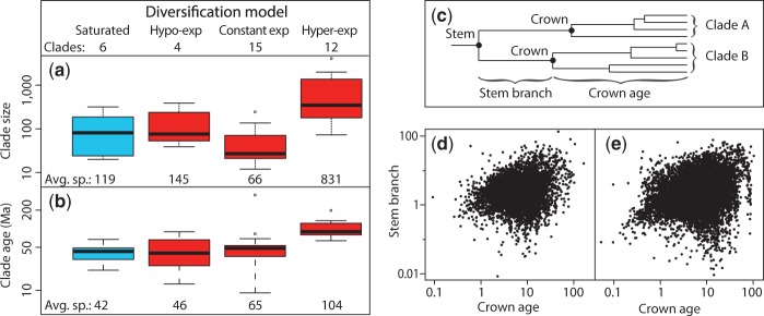
(1 column) Diversification analyses of major Linnaean clades in the timetree of life. (a–b) Results of coalescent analyses testing models of diversification. Of 48 tetrapod clades, 37 showed significant model selected and they were used in these analyses. (a) Effect of clade size (number of described species). (b) Effect of clade age. (c) Diagram illustrating difference between stem and crown age for two clades. (d–e) Relationship of stem branch and crown age in mammals (d; r² = 0.07) and birds (e; r² = 0.04).

Diversification by expansion predicts a significant correlation between clade age and clade size (see Materials and Methods). Therefore, we evaluate the expansion hypothesis in two densely sampled groups: Mammals (5,363 species) and birds (9,879 species). We also tested the effect of stem versus crown age (fig. 5c) on clade sizes (supplementary Materials and Methods, Supplementary Material online); stem age includes the time elapsed on the branch leading to the crown. We examined 1,990 clades in two separate analyses: Families (153 and 113 nonnested clades for birds and mammals, respectively) and genera (1,115 and 609 nonnested clades for birds and mammals, respectively). In each case, the relationship was highly significant for crown age (r = 0.43–0.47, P < 0.001) but nonsignificant or weakly significant (r = 0.02–0.09, P = 0.01–0.82) using stem age (see Materials and Methods). These results demonstrate a significant relationship between clade age and clade size in major groups of vertebrates, and provide an explanation why this was not observed in past studies, as they used stem ages (crown age + stem branch time).

Our results show that it is best to avoid stem branch time, because the length of any (stem) branch in the tree should not be related to the time depth of the descendant node (crown age; fig. 5d and e). Therefore, the use of stem branch time will introduce large statistical noise and make the test extremely conservative. For example, when considering every node in a timetree of species, the coefficient of variation of stem branch length relative to crown age is over 200% in the best sampled groups, mammals (208%) and birds (224%). That noise is further weighted by the pull of the present (Nee et al. 1994), which, we determined, adds 40% time (median) to crown age at any given node (if stem age is used instead of crown age), in separate analyses of birds, mammals, and all eukaryotes. This is because the pull of the present creates longer internal branches deeper in a tree, as more lineages are pruned by extinction. Therefore, the use of stem branches in diversification analyses adds noise (variance) and gives increased weight to that noise. We believe that the stronger signal of constant expansion in our results, compared with earlier studies that have supported hypo-expansion and saturation, is in part because we have identified and avoided some biases (e.g., sampling effort, clade size, and stem age) that can impact diversification analyses.

Speciation

The rate of formation of new species is the primary input into the diversification of life over time. This process starts as two or more lineages split from an existing species at a node in the tree. To learn more about the timing of speciation, we assembled a separate data set of studies containing timetrees that included populations and species of eukaryotes (supplementary Materials and Methods, Supplementary Material online). Considering a standard model of speciation based on geographic isolation, in the absence of gene flow (Sousa and Hey 2013), we estimated the time required for speciation to occur. For a given species, the time-to-speciation (TTS), after isolation, must fall between the crown and the stem age of the species (fig. 6a). All lineages younger than the crown age of a species lead to populations that are still capable of interbreeding and, therefore, must be younger than the TTS. On the other hand, the stem age is the time when a species joins its closest relative and, therefore, it must be older than the TTS. A sampling omission of either a population or species could lower the crown age estimate or raise the stem age estimate, but the resulting interval would still contain the TTS. Although coalescence of alleles may lead to overestimates of time (Nei and Kumar 2000), those times were interpreted as population and species splits, not allelic splits, in the published studies reporting them. Also, calibrations can ameliorate the effect of allelic coalescence because they are usually based on population and species divergences, not coalescence events. We conducted a simulation to test this approach (supplementary Materials and Methods, Supplementary Material online) finding that the true TTS is estimated precisely with a mode because of skewness of the statistical distribution and it is robust to undersampling of lineages, either younger (populations) or older (species). We also found that the true TTS was not affected by the addition of 10% noise (intervals that do not include the TTS) and only weakly affected (2.5%) by adding a large amount (50%) of noise.

Fig. 6.

(2 columns) Estimation of time-to-speciation. (a) Analytical design showing expected results. Intervals between stem age and crown age of seven species contain time-to-speciation (dashed line represents the modal time-to-speciation). Divergences among populations, and corresponding histogram, are in red. (b) Colored histograms of observed time-to-speciation, showing modes (vertical lines) and confidence intervals (bars) in vertebrates (N = 213, 2.1 Ma, 1.74–2.55 Ma), arthropods (N = 85, 2.2 Ma, 1.57–3.07 Ma), and plants (N = 55, 2.7 Ma, 2.37–3.63 Ma). Black curves to the right are histograms of population divergences.

Analyses of three disparate taxonomic groups (vertebrates, arthropods, and plants) with greatly varying generation times and life histories produced similar TTS of ∼2 My (fig. 6b). For comparison, divergence times among closely related species of prokaryotes, which are defined in practical terms (Cohan 2002), are about 50–100 times older (supplementary Materials and Methods, Supplementary Material online). The observed similarity of TTS in diverse groups of multicellular eukaryotes suggests a model of speciation that places importance on the time that two populations are isolated (fig. 7). If speciation is an outcome of the buildup of genic incompatibilities (GIs) between isolated populations (Coyne and Orr 2004; Matute et al. 2010), then the continuous fixation of selectively neutral mutations in two populations (Zuckerkandl and Pauling 1965; Kimura 1968) will accumulate with time and eventually lead to a number, or fraction, of GIs (here, “S-value”) that will cause postzygotic reproductive isolation (fig. 7c). In essence, speciation—in the strictest sense—can be defined as this specific moment in time, a “point of no return,” because reproductive incompatibility and isolation are inevitable at that point. The diverging lineages will remain independent forever or until they become extinct. If they do come back into contact (fig. 7a), they might hybridize briefly but would then undergo reinforcement, leading to prezygotic reproductive isolation. We focus here on the major model, geographic isolation, but time constraints should be similar with ecological speciation, and other models exist (Coyne and Orr 2004).

Fig. 7.

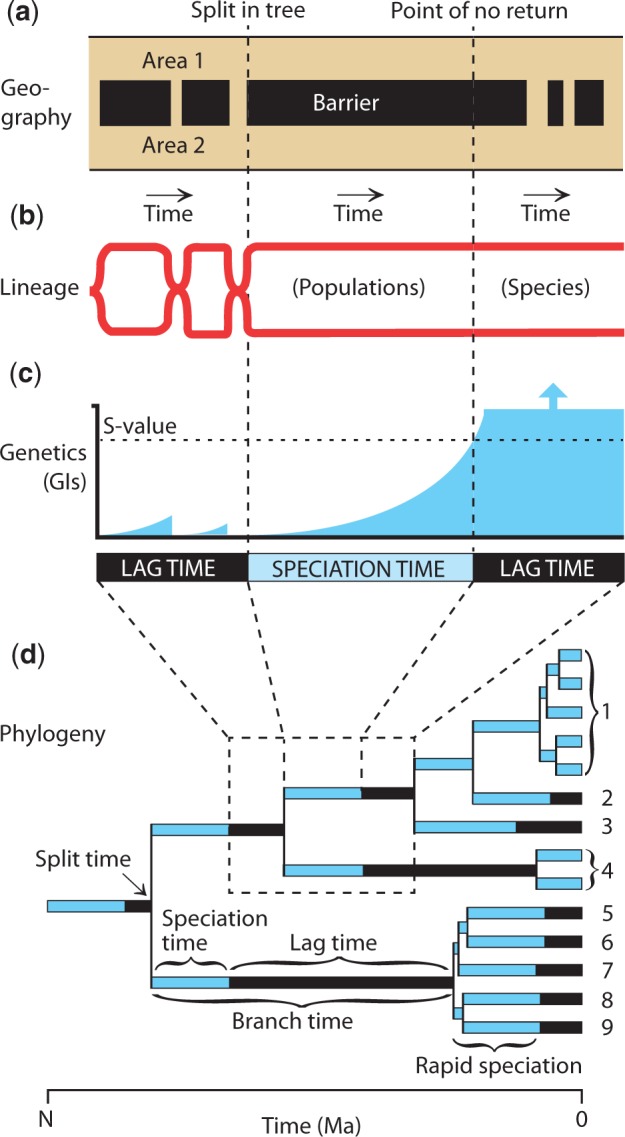
(1 column) Summary model of speciation. (a) Biogeographic history showing the contact and isolation of areas occupied by the two populations. (b) Phylogenetic lineages showing times of independence (two lineages) and times of interbreeding (one lineage). (c) Genic incompatibilities between the two populations, showing how they accrue at a time-dependent rate during geographic isolation, reset to zero during contact (interbreeding), increase to the S-value (the number of GIs that will cause speciation, the point of no return), and continue increasing beyond the S-value despite later contact of the newly formed species. (d) Hypothetical phylogeny, with numbered species, illustrating parameters of speciation in (a–c) to splits and branches in a tree.

A speciation clock has been suggested previously (Coyne and Orr 1989), where GIs buildup linearly over time in postzygotic reproductive isolation. However, current evidence indicates a faster-than-linear (“snowball”) rate of buildup of GIs in postzygotic reproductive isolation (Matute et al. 2010). The snowball pattern of increase in GIs is not a problem for a speciation clock as long as the time of attainment of the S-value is similar in different species. Our evidence from the TTS analysis (fig. 7b) suggests this to be the case.

Relatively few populations will remain isolated until the point of no return because environments often change rapidly in the short term, raising and lowering barriers to gene flow (fig. 7a). This is amplified by a preponderance of low incline landscapes (Strahler 1952), resulting in a greater impact of climate and sea level change. Therefore, the buildup of GIs will be reset many times before a successful speciation event occurs (fig. 7c). This resetting, which results in failed isolates, may explain “barcode gaps” (Puillandre et al. 2011), which we interpret as prespeciation loss of potential lineages. We estimate that branches between nodes in well-sampled (>20% coverage) groups of the TTOL are, on average, 4–5 My long using a slope method (4.92 ± 0.32 My) and a coalescent method (4.21 ± 0.76 My) (supplementary Materials and Methods, Supplementary Material online). This indicates that branch time is longer than TTS, and includes a significant “lag time,” referring to any time along a branch that is not part of a successful speciation event, such as the resetting of the speciation clock by reversal of the buildup of GIs. The high variance of branch length in trees (fig. 5d and e) may reflect the stochastic nature of environmental change and isolation of populations, contributing to a “diversification clock” (fig. 4). This is consistent with the absence of a strong correlation between reproductive isolation and diversification rate in some taxa (Rabosky and Matute 2013).

In relating this speciation model to a phylogeny (fig. 7d), it is evident that the split of two lineages in a tree is not the speciation event but rather the moment of isolation of two or more populations that will remain isolated until the point of no return. For example, if we assume a TTS of 2 My, then two populations that only recently became species would have split ∼2 Ma (fig. 7d, species 1–2). Yet, much deeper in a tree, where branches may be tens of millions of years long, the TTS is a relatively small fraction of total branch time, which makes a splitting event more-or-less equivalent to the speciation event. Furthermore, branch splitting leading to eventual species formation can happen simultaneously, in many lineages, as long as the resulting populations remain isolated until the point of no return (fig. 7d, species 5–9).

Discussion

These results have implications for patterns of species diversification and the interpretation of timetrees. If adaptation is largely decoupled from speciation, we should not expect it to be a driver of speciation as is frequently assumed. Also, we should not expect to see major diversification rate increases following mass extinction events, even though large adaptive changes took place at those times. That expectation is realized in our analyses (fig. 4) where we see constant splitting through time across the two major Phanerozoic extinction events (251 and 66 Ma). Likewise, our diversification analyses of smaller groups, such as birds and mammals (supplementary fig. S4, Supplementary Material online), and past studies of those groups (Bininda-Emonds et al. 2007; Meredith et al. 2011; Jetz et al. 2012) have not found rate increases immediately following the end-Cretaceous mass extinction event (66 Ma). Rate decreases from the extinction events themselves are not expected because of the inability to detect, in trees, a large proportion of species extinctions that occurred (Nee and May 1997).

The consistency in TTS among groups found here suggests that the time-based acquisition of GIs, and not adaptive change, is driving reproductive isolation, almost in a neutral process. By implication, geographically isolated populations, even if morphologically different and diagnosable, are not expected to be species until they have reached the point of no return. This is because some differentiation and adaptive change should occur in isolation, and many isolates will be ephemeral (Rosenblum et al. 2012), merging with other isolates or disappearing and never becoming species that enter the tree of life. More population data are needed before it is possible to identify the point of no return with precision. Nonetheless, these data suggest that, in most cases, described species separated by only tens of thousands of years are not real species. The Linnaean rank of subspecies, which has declined in use for decades, might be appropriate for such diagnosable isolates that have not yet reached the point of no return. Oversplitting of species by taxonomists may explain the sharp peak in diversification (hyper-expansion) in the last 10 My of eukaryote history (fig. 4b). On the other hand, it could also result from statistical (small sample) artifacts that were published in many different studies (summarized in the TTOL). Therefore, further analysis of that unusual rate spike is warranted.

In summary, the diversification of life as a whole is expanding at a constant rate and only in some small clades (<500 species) is there evidence of decline or saturation in diversification rate. We believe these results can be explained as many different groups of organisms undergoing expansion and contraction through time, with those patterns captured in different stages (expanding, slowing, or in equilibrium). If true, the predominant pattern of expansion in large clades is expected from the law of large numbers, where such smaller, random events would average to a constant rate. Constant expansion also follows from random environmental changes leading to isolation and speciation. Rate constancy is consistent with the fossil record (Benton 2009) and does not deny the importance of biotic factors in evolution (Ricklefs 2007), but it suggests an uncoupling of speciation and adaptation. Cases where the phenotype has changed little (e.g., cryptic species) or greatly during the TTS are interpreted here as evidence of uncoupling. The lineage splitting seen in trees probably reflects, in most instances, random environmental events leading to isolation of populations, and potentially many in a short time. However, the relatively long TTS (∼2 My), a process resulting from random genetic events, will limit the number of isolates that eventually become species. Under this model, diversification is the product of those two random processes, abiotic and genetic, and rate increases (bursts of speciation) are more likely to be associated with long-term changes in the physical environment (e.g., climate, sea level) causing extended isolation rather than with short-term ecological interactions. However, reductions in extinction rate could also explain increases in diversification rate. Adaptive change that characterizes the phenotypic diversity of life would appear to be a separate process from speciation. Although a full understanding of these processes remains a challenge, determining how speciation and adaptation are temporally related would be an important “next step.”

Materials and Methods

Detailed methods are described in supplementary Materials and Methods, Supplementary Material online.

TTOL Data Collection

We synthesized the corpus of scientific literature where the primary research on the TTOL is published. We first identified and collected all peer-reviewed publications in molecular evolution and phylogenetics that reported estimates of time of divergence among species. These included phylogenetic trees scaled to time (timetrees) and occasionally tables of time estimates and regular text. We assembled timetree data from 2,274 studies (http://www.timetree.org/reference_list.php ) that have been published between 1987 and April 2013, as well as two timetrees estimated herein (supplementary table S1, Supplementary Material online). Most (96%) of nodal times used were published in the last decade.

TTOL Analytics and Synthesis

We used a hierarchical average linkage method of estimating divergence times (T_s) of clade pairs to build a Super Timetree, along with a procedure for testing and updating topological partitions to ensure the highest degree of consistency with individual timetrees in every study. For the TTOL, uncertainty derived from individual studies is available for each node (supplementary table S2, Supplementary Material online). Branch time modes of different Linnaean categories were estimated (supplementary table S3, Supplementary Material online).

Diversification Analyses

All diversification analyses were performed in R (http://www.r-project.org/) with the APE package (Paradis et al. 2013). The gamma statistic was employed to detect decrease in speciation rate over the history of the tree. To test if diversification is saturated or expanding, we used a coalescent method as well as the relationship between the ages of different clades and their sizes (numbers of species). The number and location of shifts in diversification rates were also tested. We also estimated among-study uncertainty in both the lineages-through-time (LTT) curve and rate test by producing 500 replicates of the TTOL, sampling actual study times at each node randomly. These replicates were then used in the analysis of rate shifts to estimate and test rate change. Results of all diversification analyses were summarized (supplementary tables S4–S10, Supplementary Material online).

Gamma Test

The gamma statistic (Pybus and Harvey 2000) was employed on 59 clades (all eukaryotes plus 58 clades listed in supplementary table S5, Supplementary Material online) to detect decrease in speciation rate over the history of the tree (LASER package; Rabosky and Schliep 2013). These 58 groups were chosen to have an overview of the diversification processes on a diversity of clades across life, in terms of size, sampling effort (above 5%; median 66%, with 84% of the clades having more than 40% coverage), and clade age. Included in the 58 clades are 10 nonnested groups over the major Linnaean groups, which allowed us to draw conclusions about high-level and low-level clades. We further selected 10 nonnested clades from within each of the four well-sampled groups of tetrapods (amphibians, birds, mammals, and squamates). We also analyzed separately the Eukaryote clade because all the other groups are nested within this one.

A negative gamma value reveals a concentration of branching times near the root, meaning a decelerated diversification. Incomplete lineage sampling can affect the result of this test because some tips will be pruned, thus lengthening the branch length in the more recent past (Nee et al. 1994). An incomplete sampling could therefore lead to an erroneous detection of slowdown. To avoid this bias, the Monte Carlo constant rate test (MCCR test) (Pybus and Harvey 2000) was also performed on clades with a significant negative gamma value (LASER package). Here, the critical value for rejecting a constant rate (α = 0.05) was calculated by examining the distribution of gamma for simulated trees with the same incomplete lineage sampling proportion as the observed tree. We conducted 5,000 Monte Carlo simulations for each MCCR test. If the MCCR test finds that the detection of slowdown is erroneous, then there is no support for decline in speciation rate for this clade.

Models of Diversification

To test if diversification is saturated or expanding, we used a coalescent method (Morlon et al. 2010) on 58 clades (supplementary table S5, Supplementary Material online). We defined two sets of models: Saturated diversity (models 1 and 2) and expanded diversity (models 3, 4a, 4b, 4c, 4d, 5, and 6). As recommended by the author of the method, we first selected the model with the lowest second-order Akaike's Information Criterion in each subset (saturated vs. expanding models). We then evaluated the relative probability of these two models based of their Akaike weights. The relative probabilities of two models (l and k) were calculated as $\frac{wl}{wl+wk}$ and $\frac{wk}{wl+wk}$, with wl (the model’s l Akaike weight) as $wl=\frac{\exp \left(-▵l/2\right)}{{\sum }_{r=1}^R\exp \left(-▵r/2\right)}$and R the number of candidate models. This method can account for missing species. We therefore used the number of described species (supplementary table S5, Supplementary Material online) as the number of tips of the phylogenies (N₀). When neither of the two relative probabilities obtained exceeded 0.6, we did not draw a conclusion on this specific clade (referred as “nonsignificant” in supplementary table S5, Supplementary Material online) and the mean λ (between the best expanding and saturating model) was used (supplementary table S4, Supplementary Material online). Statistical tests were performed (supplementary table S6, Supplementary Material online) to compare the four models, saturated (sat), hyper-expanding (exp+), expanding (exp), and hypo-expanding (exp-), at the same time (Kruskall–Wallis rank-sum test) and by pair (Wilcoxon rank-sum test). Another test was performed (t-test) to compare the means (described number of species and crown age) between the clades under hyper-expansion and the others (saturated, hypo-expanding, and expanding). We confirmed for all clades that the BD polytomy resolution did not change the results, although a different model was selected for 3 of the 58 clades (5%). This method was computationally unfeasible with the entire TTOL.

Clade Age and Clade Size Analyses

To test, in another way, for expansion (hyper-, constant-, and hypo-) versus saturation of the diversification curve, we evaluated the relationship between the ages of different clades and their sizes (numbers of species) (Cornell 2013). Under the saturated diversity model, no relationship should be observed, in contrast to a positive relationship under models of expanding diversity. For this test, we chose the two best sampled groups, birds and mammals, and performed comparative analyses on clades (all nonnested) of genera (1,115 and 609 for birds and mammals respectively) and families (153 and 113 for birds and mammals, respectively), accounting for phylogeny (phylogenetic generalized linear models) with the CAPER package (Orme et al. 2013). In one set of analyses, we used stem age and in another set, crown age (supplementary table S7, Supplementary Material online) was used.

Detection of Shifts in Diversification Rates

The TREEPAR package (Stadler 2013) was used to estimate the number of changes in diversification rate under a BD model and to obtain estimates of the corresponding diversification rate (λ−μ) and the extinction fraction (μ/λ). To analyze our eukaryote timetree, as well as the individual component timetrees of birds and mammals, we used the greedy approach, as described in Stadler (2011). We estimated rates in 0.1 My steps between 2 and 70 Ma and in 10 My steps between 2 and 3,500 My for eukaryotes. The BD shift model (without mass extinction) was used and we obtained maximum-likelihood rate estimates for the different data sets for zero, one, two, three, four, five, six, and seven rate shifts. The likelihood ratio test was used to select the best model in each case at the 99% level.

For the TTOL, we estimated node time uncertainty in both the LTT curve and rate test by producing 500 replicates of the TTOL, sampling a time between the confidence intervals at each node under a uniform distribution. These replicates were then used in the TREEPAR analysis to estimate and test rate change, with the uncertainty shown in figure 4 and the significant shifts by time interval (20 My) shown in supplementary table S8, Supplementary Material online.

Our diversification results for birds are similar to an earlier analysis (Jetz et al. 2012), with a strong increase in diversification from ∼45 Ma to the present. The mammal results are also generally similar to past mammal analyses in showing the absence of any rate increase immediately after the end-Cretaceous extinctions (Bininda-Emonds et al. 2007; Meredith et al. 2011). We did not find a sharp mid-Cenozoic increase in rate that was found in one other analysis (Stadler 2011), although we determined that the cause of that rate increase was from a polytomy in the mammal timetree used in that study (Stadler 2011); otherwise our results are comparable.

For the bird tree (supplementary fig. S4a, Supplementary Material online), the models with zero, one, two, three, four, and five rate shifts are rejected in favor of a model with six rate shifts (P < 0.05) (supplementary table S9, Supplementary Material online). A model with six rate shifts is not rejected in favor of a model with seven rate shifts (P = 0.091). The 6 shifts are detected at 1, 3.4, 14.4, 48.2, 73.3, and 84.4 Ma (supplementary table S10, Supplementary Material online). The parameters obtained for the 6 shifts model between 73.3 and 48.2 Ma (λ−μ = 0.04058 and μ/λ = 0.0395) were used to plot the confidence interval of the null distribution (supplementary fig. S4a, Supplementary Material online).

For the mammal tree (supplementary fig. S4b, Supplementary Material online), the models with zero, one, two, or three rate shifts are rejected in favor of a model with four rate shifts (P < 0.05) (supplementary table S9, Supplementary Material online). A model with four rate shifts is not rejected in favor of a model with five rate shifts (P = 0.123). The 4 shifts are detected, at 2.1, 9.6, 42.4 and 105 Ma (supplementary table S10, Supplementary Material online). The parameters obtained for the 4 shifts model between 105 and 42.4 Ma (λ−μ = 0.05186 and μ/λ = 0.3528) were used to plot the confidence interval of the null distribution (supplementary fig. S4b, Supplementary Material online).

For the eukaryote tree (fig. 4), the models with zero, one, two, three, four, and five rate shifts are rejected in favor of a model with six rate shifts (P < 0.05) (supplementary table S9, Supplementary Material online). A model with six rate shifts is not rejected in favor of a model with seven rate shifts (P = 0.055). Six shifts are thus detected at 1, 11, 21, 121, 14,1 and 151 Ma (supplementary table S10, Supplementary Material online). The parameters obtained for the 6 shifts model between 2,100 and 151 Ma (λ−μ = 0.00307 and μ/λ = 0.9581) were used to plot the confidence interval of the null distribution (fig. 4).

In addition, we used the BAMMtools package (Rabosky 2014) in order to detect the diversification rate differences across lineages. The function “setBAMMpriors” was used to generate a prior block that matched the “scale” (e.g., depth of the tree) of our data. Both the speciation and the extinction rate were allowed to vary through time and across lineages, and 50,000,000 generations of MCMC simulation were performed. The sampling fraction (0.02635422) was specified by setting the “globalSamplingFraction” parameter. A burnin of 0.5 was applied and a diversification rate plot was obtained with the function “plotRateThroughTime” (supplementary fig. S3, Supplementary Material online).

Time-to-Speciation Analyses

In addition to our species-level TTOL data collection described above, we collected a separate data set on TTS from published molecular timetrees that included timed nodes among populations and closely related species of three major groups: Vertebrates, arthropods, and plants (supplementary tables S11–S13, Supplementary Material online). To test the robustness of our approach for estimating TTS, we used simulations. A BD tree was simulated using the function “sim.bd.taxa” (TreeSim in R).

Supplementary Material

Supplementary figures S1–S4, tables S1–S13, and Materials and Methods are available at Molecular Biology and Evolution online (http://www.mbe.oxfordjournals.org/).

References

- Avise JC, Liu JX. On the temporal inconsistencies of Linnean taxonomic ranks. Biol J Linn Soc. 2011;102(4):707–714. [Google Scholar]
- Battistuzzi FU, Billing-Ross P, Paliwal A, Kumar S. Fast and slow implementations of relaxed-clock methods show similar patterns of accuracy in estimating divergence times. Mol Biol Evol. 2011;28(9):2439–2442. doi: 10.1093/molbev/msr100. [DOI] [PMC free article] [PubMed] [Google Scholar]
- Benton MJ. The Red Queen and the Court Jester: species diversity and the role of biotic and abiotic factors through time. Science. 2009;323(5915):728–732. doi: 10.1126/science.1157719. [DOI] [PubMed] [Google Scholar]
- Bininda-Emonds OR, Cardillo M, Jones KE, MacPhee RD, Beck RM, Grenyer R, Price SA, Vos RA, Gittleman JL, Purvis A. The delayed rise of present-day mammals. Nature. 2007;446(7135):507–512. doi: 10.1038/nature05634. [DOI] [PubMed] [Google Scholar]
- Cohan FM. What are bacterial species? Ann Rev Microbiol. 2002;56:457–487. doi: 10.1146/annurev.micro.56.012302.160634. [DOI] [PubMed] [Google Scholar]
- Cornell HV. Is regional species diversity bounded or unbounded? Biol Rev. 2013;88(1):140–165. doi: 10.1111/j.1469-185X.2012.00245.x. [DOI] [PubMed] [Google Scholar]
- Costello MJ, May RM, Stork NE. Can we name Earth's species before they go extinct? Science. 2013;339(6118):413–416. doi: 10.1126/science.1230318. [DOI] [PubMed] [Google Scholar]
- Coyne JA, Orr HA. Patterns of speciation in Drosophila. Evolution. 1989;43(2):362–381. doi: 10.1111/j.1558-5646.1989.tb04233.x. [DOI] [PubMed] [Google Scholar]
- Coyne JA, Orr HA. 2004 Speciation. Sunderland (MA): Sinauer Associates, Inc. [Google Scholar]
- Cusimano N, Renner SS. Slowdowns in diversification rates from real phylogenies may not be real. Syst Biol. 2010;59(4):458–464. doi: 10.1093/sysbio/syq032. [DOI] [PubMed] [Google Scholar]
- Etienne RS, Rosindell J. Prolonging the past counteracts the pull of the present: protracted speciation can explain observed slowdowns in diversification. Syst Biol. 2012;61(2):204–213. doi: 10.1093/sysbio/syr091. [DOI] [PMC free article] [PubMed] [Google Scholar]
- Hedges SB, Dudley J, Kumar S. TimeTree: a public knowledge-base of divergence times among organisms. Bioinformatics. 2006;22(23):2971–2972. doi: 10.1093/bioinformatics/btl505. [DOI] [PubMed] [Google Scholar]
- Hedges SB, Kumar S. The timetree of life. Oxford: Oxford University Press; 2009. [Google Scholar]
- Hoffmann M, Hilton-Taylor C, Angulo A, Bohm M, Brooks TM, Butchart SH, Carpenter KE, Chanson J, Collen B, Cox NA, et al. The impact of conservation on the status of the world's vertebrates. Science. 2010;330(6010):1503–1509. doi: 10.1126/science.1194442. [DOI] [PubMed] [Google Scholar]
- Jetz W, Thomas GH, Joy JB, Hartmann K, Mooers AO. The global diversity of birds in space and time. Nature. 2012;491(7424):444–448. doi: 10.1038/nature11631. [DOI] [PubMed] [Google Scholar]
- Kimura M. Evolutionary rate at the molecular level. Nature. 1968;217:624–626. doi: 10.1038/217624a0. [DOI] [PubMed] [Google Scholar]
- Matute DR, Butler IA, Turissini DA, Coyne JA. A test of the snowball theory for the rate of evolution of hybrid incompatibilities. Science. 2010;329(5998):1518–1521. doi: 10.1126/science.1193440. [DOI] [PubMed] [Google Scholar]
- Meredith RW, Janecka JE, Gatesy J, Ryder OA, Fisher CA, Teeling EC, Goodbla A, Eizirik E, Simao TLL, Stadler T, et al. Impacts of the Cretaceous Terrestrial Revolution and KPg extinction on mammal diversification. Science. 2011;334(6055):521–524. doi: 10.1126/science.1211028. [DOI] [PubMed] [Google Scholar]
- Moen D, Morlon H. Why does diversification slow down? Trends Ecol Evol. 2014;29(4):190–197. doi: 10.1016/j.tree.2014.01.010. [DOI] [PubMed] [Google Scholar]
- Morlon H. Phylogenetic approaches for studying diversification. Ecol Lett. 2014;17:508–525. doi: 10.1111/ele.12251. [DOI] [PubMed] [Google Scholar]
- Morlon H, Potts MD, Plotkin JB. Inferring the dynamics of diversification: a coalescent approach. PLoS Biol. 2010;8(9):e1000493. doi: 10.1371/journal.pbio.1000493. [DOI] [PMC free article] [PubMed] [Google Scholar]
- National Center for Biotechnology Information. 2013 Taxonomy Browser. Bethesda (MD): National Center for Biotechnology Information [Cited 2014 Nov 21]. Available from: http://www.ncbi.nlm.nih.gov/ [Google Scholar]
- Nee S, May RM. Extinction and the loss of evolutionary history. Science. 1997;278(5338):692–694. doi: 10.1126/science.278.5338.692. [DOI] [PubMed] [Google Scholar]
- Nee S, May RM, Harvey PH. The reconstructed evolutionary process. Philos Trans R Soc B. 1994;344(1309):305–311. doi: 10.1098/rstb.1994.0068. [DOI] [PubMed] [Google Scholar]
- Nei M. Mutation driven evolution. New York: Oxford University Press; 2013. [Google Scholar]
- Nei M, Kumar S. Molecular evolution and phylogenetics. New York: Oxford University Press; 2000. [Google Scholar]
- Orme D, Freckleton R, Thomas G, Petzoldt T, Fritz S, Isaac N, Pearse W. 2013 Caper: comparative analyses of phylogenetics and evolution in R. Vienna (Austria): Comprehensive R Archive Network [Cited 2014 Nov 21]. Available from: http://CRAN.R-project.org/package=caper. [Google Scholar]
- Paradis E, Bolker B, Claude J, Cuong HS, Desper R, Durand B, Dutheil J, Gascuel O, Heibl C, Lawson D, et al. 2013 Ape: analyses of phylogenetics and evolution. Vienna (Austria): Comprehensive R Archive Network [Cited 2014 Nov 21]. Available from: http://CRAN.R-project.org/package=ape. [Google Scholar]
- Puillandre N, Lambert A, Brouillet S, Achaz G. ABGD, Automatic Barcode Gap Discovery for primary species delimitation. Mol Ecol. 2011;21:1864–1877. doi: 10.1111/j.1365-294X.2011.05239.x. [DOI] [PubMed] [Google Scholar]
- Pybus OG, Harvey PH. Testing macro-evolutionary models using incomplete molecular phylogenies. Proc R Soc Lond B Biol Sci. 2000;267(1459):2267–2272. doi: 10.1098/rspb.2000.1278. [DOI] [PMC free article] [PubMed] [Google Scholar]
- Rabosky DL. Diversity-dependence, ecological speciation, and the role of competition in macroevolution. Annu Rev Ecol Evol Syst. 2013;44:481–502. [Google Scholar]
- Rabosky DL. Automatic detection of key innovations, rate shifts, and diversity-dependence on phylogenetic trees. PLoS One. 2014;9:e89543. doi: 10.1371/journal.pone.0089543. [DOI] [PMC free article] [PubMed] [Google Scholar]
- Rabosky DL, Matute DR. Macroevolutionary speciation rates are decoupled from the evolution of intrinsic reproductive isolation in Drosophila and birds. Proc Natl Acad Sci U S A. 2013;110(38):15354–15359. doi: 10.1073/pnas.1305529110. [DOI] [PMC free article] [PubMed] [Google Scholar]
- Rabosky DL, Schliep K. 2013 LASER: a maximum likelihood toolkit for detecting temporal shifts in diversification rates from molecular phylogenies. Vienna (Austria): Comprehensive R Archive Network [Cited 2014 Nov 21]. Available from: http://cran.r-project.org/package=laser. [Google Scholar]
- Rabosky DL, Slater GJ, Alfaro ME. Clade age and species richness are decoupled across the Eukaryotic tree of life. PLoS Biol. 2012;10(8):e1001381. doi: 10.1371/journal.pbio.1001381. [DOI] [PMC free article] [PubMed] [Google Scholar]
- Ricklefs RE. Estimating diversification rates from phylogenetic information. Trends Ecol Evol. 2007;22(11):601–610. doi: 10.1016/j.tree.2007.06.013. [DOI] [PubMed] [Google Scholar]
- Rosenblum EB, Sarver BAJ, Brown JW, Roches SD, Hardwick KM, Hether TD, Eastman JM, Pennell MW, Harmon LJ. Goldilocks meets Santa Rosalia: an ephemeral speciation model explains patterns of diversification across time scales. Evol Biol. 2012;39:255–261. doi: 10.1007/s11692-012-9171-x. [DOI] [PMC free article] [PubMed] [Google Scholar]
- Sepkoski JJ. A kinetic model of Phanerozoic taxonomic diversity. 3. Post-Paleozoic families and mass extinctions. Paleobiology. 1984;10(2):246–267. [Google Scholar]
- Smith SA, O'Meara BC. treePL: divergence time estimation using penalized likelihood for large phylogenies. Bioinformatics. 2012;28(20):2689–2690. doi: 10.1093/bioinformatics/bts492. [DOI] [PubMed] [Google Scholar]
- Sousa V, Hey J. Understanding the origin of species with genome-scale data: modelling gene flow. Nat Rev Genet. 2013;14(6):404–414. doi: 10.1038/nrg3446. [DOI] [PMC free article] [PubMed] [Google Scholar]
- Stadler T. Mammalian phylogeny reveals recent diversification rate shifts. Proc Natl Acad Sci U S A. 2011;108(15):6187–6192. doi: 10.1073/pnas.1016876108. [DOI] [PMC free article] [PubMed] [Google Scholar]
- Stadler T. 2013 TreePar: estimating birth and death rates based on phylogenies. Vienna (Austria): Comprehensive R Archive Network [Cited 2014 Nov 21]. Available from: http://CRAN.R-project.org/package=TreePar. [Google Scholar]
- Strahler AN. Hypsometric (area-altitude) analysis of erosional topography. Geol Soc Am Bull. 1952;63:1117–1142. [Google Scholar]
- Tamura K, Battistuzzi FU, Billing-Ross P, Murillo O, Filipski A, Kumar S. Estimating divergence times in large molecular phylogenies. Proc Natl Acad Sci U S A. 2012;109(47):19333–19338. doi: 10.1073/pnas.1213199109. [DOI] [PMC free article] [PubMed] [Google Scholar]
- Venditti C, Meade A, Pagel M. Phylogenies reveal new interpretation of speciation and the Red Queen. Nature. 2010;463(7279):349–352. doi: 10.1038/nature08630. [DOI] [PubMed] [Google Scholar]
- Zuckerkandl E, Pauling L. Evolutionary divergence and convergence in proteins. In: Bryson V, Vogel HJ, editors. Evolving genes and proteins. New York: Academic Press; 1965. pp. 97–165. [Google Scholar]
Associated Data
This section collects any data citations, data availability statements, or supplementary materials included in this article.