Optimal Point Spread Function Design for 3D Imaging

Abstract

To extract from an image of a single nanoscale object maximum physical information about its position, we propose and demonstrate a framework for pupil-plane modulation for 3D imaging applications requiring precise localization, including single-particle tracking and super-resolution microscopy. The method is based on maximizing the information content of the system, by formulating and solving the appropriate optimization problem – finding the pupil-plane phase pattern that would yield a PSF with optimal Fisher information properties. We use our method to generate and experimentally demonstrate two example PSFs: one optimized for 3D localization precision over a 3 μm depth of field, and another with an unprecedented 5 μm depth of field, both designed to perform under physically common conditions of high background signals.

Optical imaging of single nanoscale objects such as a quantum dot, metallic nanoparticle, or a single molecule provides a powerful window into a variety of biological or material systems, and the physical problem of extracting maximum information from single emitters is an important goal. One application is single-particle tracking (SPT [1]), which relies upon extracting the spatial trajectory of a single moving molecular label, quantum dot, or metallic nanoparticle from a series of images. For example, a single mRNA particle can be localized and followed in a living cell in real-time [2]. Another application of single-molecule localization is “super-resolution” (SR) microscopy, [3–5] which works by ensuring that only a sparse subset of labels on an extended object (e.g. a cellular structure) are emitting in each imaging frame. One localizes the single emitters just as in SPT; the multitude of localizations are then reconstructed into a single, high-resolution image. This enables the spatial resolving power of SR microscopy to surpass the classical diffraction resolution limit by 5- to 10-fold.

Historically, single-particle localization was used for 2D imaging, namely, inferring the x,y coordinates of each emitter, e.g. by centroid-fitting of by fitting to a 2D Gaussian [6]. However, the third spatial dimension, z, or the depth of an emitter, can also be inferred from its measured 2D image. This can be done by considering how the shape of the microscope’s point spread function (PSF) varies with emitter position. The PSF of a microscope is the image that is detected when observing a point source. For a standard microscope, to a good approximation, the PSF in focus (i.e. z=0) resembles a circular Airy pattern, and its shape is invariant to lateral shifts (x,y) of the emitter – however it will change upon defocus (z). Unfortunately, the standard PSF spreads out (defocuses) quickly with z which limits the range over which z can be determined.

Importantly, to obtain much more useful 3D position information, the PSF of the microscope can be altered – for example by pupil (Fourier) plane processing [7,8]. Phase modulating the electromagnetic field in the Fourier plane is a low-loss method to encode z-information in the shape of the image on the camera. Examples of this include astigmatic PSFs [9,10], double-helix (DH-PSF) microscopy [11–13] or segmented phase ramps [14].

The precision to which a single emitter can be localized depends on several factors. These include the emitter’s brightness (detected photon flux), background fluorescence, detector pixel size, and detection noise [15,16]. Another key factor is the shape of the PSF itself. For example, in astigmatism-based 3D imaging, the PSF is altered to have an elliptical shape, and the z position of the emitter can be determined by the relative widths of the PSF along the two principal axes [9,10]. The double-helix PSF [12,13] is composed of two spots, with the angle between a line connecting them and the camera axis encoding the z position of the emitter. Among existing PSFs for 3D imaging, the double-helix PSF has been shown to allow a larger depth of field than astigmatism (~2–3 μm vs ~0.5–0.7 μm) [17], and a recently suggested PSF based on accelerating beams [18] demonstrates high, uniform precision over a 3 μm range. The purpose of this paper is to fundamentally improve upon these previous schemes.

Here, we address the problem of finding a feasible and optimally informative PSF. Namely, we ask the question – given an imaging scenario with certain characteristics (e.g. magnification, noise level, pixel size, emitter signal) – what is the pupil plane pattern that would yield maximal physical information about the 3D position of an emitter, and what is the resulting optimal PSF? In other words – since localization precision depends on the PSF of the system – can we design the system to have a PSF that would yield the best possible precision in determining x, y, and z, compared to any other PSF? We regard such a PSF as optimally informative.

A powerful measure of the effectiveness of a PSF for encoding an emitter’s position is based on Fisher information [17,19,20], a concept from statistical information theory. Fisher information is a mathematical measure of the sensitivity of an observable quantity (the PSF) to changes in its underlying parameters (emitter position). Using the Fisher information function, one may compute the Cramér-Rao lower bound (CRLB), which is the theoretical best-case x,y,z precision that can be attained (with any unbiased estimator) given a PSF and a noise model. With the right estimator, the best-case localization precision represented by the CRLB can be approached in practice [21–23]. Traditionally, the CRLB has been used as an analysis tool, i.e. to evaluate the performance of an existing PSF design, which is often conceived using physical intuition and reasonable requirements (e.g. a significant change of the PSF over the z-range of interest, and concentration of emitted light into small spots). The CRLB has also been used to fine-tune an existing PSF [24].

To find the optimal pupil plane pattern, and thereby the optimal PSF, we propose a new approach to PSF design –we treat the PSF as a free design parameter of the imaging system, and generate PSFs with optimal photon-efficient 3D position encoding, with no prior constraints on the shape of the PSF. This is achieved by CRLB optimization – that is, we directly solve the mathematical optimization problem of minimizing the CRLB (and hence improving the precision bound) of the system, and use the resulting PSF. Such a PSF will provide optimal precision by definition. Physically reasonable requirements are accounted for by using realistic imaging and noise models, including pixelation, photon shot-noise Poisson statistics, and background fluorescence. This enables us to demonstrate, for typical experimental conditions and without scanning, the highest theoretical precision to date over a 3 μm axial range, as well as <50 nm experimental precision for an unprecedented ~5 μm range.

Fisher Information and CRLB

Single-emitter localization is in essence an estimation problem: Given a noisy and pixelated measurement of a PSF, the goal is to estimate the 3D position of the emitter. The Fisher information matrix [17,20] describes the sensitivity of a measurement (in our case – the PSF) to the parameters being estimated (emitter position). It is defined as:

$${\mathrm{I}}_{\text{ij}}(\mathit{\theta })=-\mathrm{E}{\left(\frac{{\partial }^{2}ln\left(\mathrm{f}\left(s;\mathit{\theta }\right)\right)}{\partial {\theta }_{\mathrm{i}}\partial {\theta }_{\mathrm{j}}}\right)}^2,$$ (1)

where θ represents the vector of parameters being estimated, f(s;θ) is the probability density, i.e. the probability of measuring a signal s given the underlying parameter vector θ and E stands for the expected value.

In our case, the signal s corresponds to the measured PSF. This measurement is assumed to be corrupted by noise, and further pixelated by the integration of intensity over the finite size of each detector pixel. The vector of underlying parameters in our case is given by θ = (x, y, z, N_ph, β), corresponding to the 3D position of the emitter, the total signal photons, and the mean background level per pixel, respectively. The probability density f(s;θ) is derived from the imaging and noise model, as follows: Each pixel in the measured image represents detected photons; theoretically this is modeled by a Poisson distributed variable, with its expected value equal to the model PSF in that pixel, as well as additive Poisson noise with a mean of β photons per pixel, due to background fluorescence. In this case, the Fisher information is a 5×5 matrix, given explicitly by [25]:

$${\mathrm{I}}_{\text{ij}}(\mathit{\theta })=\sum _{\mathrm{k}=1}^{{\mathrm{N}}_{\mathrm{p}}}\frac{1}{{\mathrm{\mu }}_{\mathrm{\theta }}(\mathrm{k})+\mathrm{\beta }}\left(\frac{\partial {\mathrm{\mu }}_{\mathrm{\theta }}(\mathrm{k})}{\partial {\theta }_{\mathrm{i}}}\right)\left(\frac{\partial {\mathrm{\mu }}_{\mathrm{\theta }}(\mathrm{k})}{\partial {\theta }_{\mathrm{j}}}\right),$$ (2)

where μ_θ(k) is the value of the model PSF in pixel k, and N_p is the number of pixels in the measurement. The diagonal of the inverse of the Fisher information matrix yields the CRLB vector, which bounds the variance of any unbiased estimator θ̂ [20] by:

$${\sigma }_{\mathrm{i}}^2=\mathrm{E}{\left({\widehat{\theta }}_i-{\theta }_i\right)}^2\ge {\left[{(\mathrm{I}(\mathit{\theta }))}^{-1}\right]}_{ii}\equiv {\text{CRLB}}_{\mathrm{i}}$$ (3)

The calculated CRLB can be compared to simulated or experimentally measured quantities as follows. For example, one can simulate or measure many images of a small static emitter, estimate its position (x/y/z) from each image, and calculate the variance of the estimations. This variance is theoretically bounded from below by (CRLB₁/CRLB₂/CRLB₃).

The Imaging Model

The 3D shape of a system’s PSF is defined by pupil-plane alteration of the optical electromagnetic field [8,12,13,26]. Concretely, a regular microscope is augmented by a 4f system [7], with a phase mask placed in the Fourier plane (Fig. 1). In the electromagnetic scalar approximation, the resulting PSF in the detector plane I(u,v) satisfies [7]:

$$I(u,v;x,y,z)\propto {\left|\mathcal{F}\right\{\mathrm{E}(x^{\prime },y^{\prime };x,y,z)·\mathrm{P}(x^{\prime },y^{\prime })\left\}\right|}^2,$$ (4)

where E(x′,y′) is the electric field in the pupil plane, caused by a point source at x,y,z, which is the 3D position relative to the focal plane and the optical axis. The complex function P(x′,y′) is the modulation function, or pattern, imposed in the pupil plane, by a specifically designed transmissive mask or a controllable spatial light modulator (SLM). We denote by the 2D spatial Fourier transform. The coordinate scaling is such that camera coordinates (u,v) correspond to Fourier plane frequencies (u/λf, v/λf), where λ is the wavelength, and f is the focal distance of the 4f lens. For details see [27].

FIG 1.

(Color online): Experimental pupil plane modulation setup with a phase mask in the Fourier plane of a 4f optical processing unit.

The Optimization Problem

The optimization problem at hand is finding a pupil plane function P(x′,y′) that yields a PSF with optimal CRLB characteristics. Because the square root of the CRLB of a PSF corresponds to the limit of attainable precision (Eq. 3), we require that the optimization produce minimal mean $\sqrt{\text{CRLB}}$ (over x, y and z) over a z-range of 3 μm; this defines our objective or cost function. We use realistic parameters for noisy biological cellular imaging data as encountered in SPT or SR imaging (2000 detected signal photons per molecule per frame, mean of β=28 background photons per pixel). Mathematically, the optimization problem is formulated as:

$$\underset{\mathrm{P}(x^{\prime },y^{\prime })}{min}\sum _{\mathrm{i}=\widehat{x},\widehat{y},\widehat{z}}\sum _{z^{\prime }\in \mathrm{Z}}\sqrt{{\text{CRLB}}_{\mathrm{i}}(z^{\prime })},$$ (5)

with the range Z ≡ [−1.5μm, 1.5μm]. Practically, we optimize over a discrete set of z positions, consisting of 250 nm increments within the range Z (a finer sampling grid did not change the results significantly). We further consider the practical constraint that P(x′,y′) is obtained using a phase-only SLM, imposing the constraint |P(x′, y′)| = 1 ∀x′, y′. This is necessary to conserve photons – a single-molecule emitter, for example, generates a finite number of photons before irreversible photobleaching.

Although it is possible in principle to optimize the phase at each one of the SLM’s 512×512 pixels separately, for practical reasons we optimize over a much more compact set of design parameters, consisting of the first 55 Zernike modes [28]. The optimization problem in Eq. (5) is non-convex, and a global minimum is not guaranteed to be found. We therefore initiate the optimization routine several times, starting from random initial values, and pick the final outcome with the minimal objective value. The optimization problem is solved using the interior-point method of Matlab’s fmincon function.

Results

The optimal solution, generated automatically by our optimization routine and shown in Fig. 2a, is the resulting pupil plane phase pattern, termed the Saddle-point (SP) mask due to its Fourier-plane shape. Figure 2b shows the numerically calculated SP-PSF corresponding to the saddle-point mask in the simulated imaging system. The dominant features of the SP-PSF are two strong lobes with varying distance and angle as a function of emitter depth (z). Figure 2c shows calculated x, y, and z $\sqrt{\text{CRLB}}$ for the SP mask, compared to two commonly used PSFs – the double-helix PSF [12,13,29] and astigmatism [9,10]. The calculation is based on the Poisson-noise corrupted model with constant background [27], with 3500 signal photons, and β = 50. In order to account for excess electron-multiplying CCD (EMCCD) noise, the quantum efficiency is adjusted as in [30] to 0.55, to match our setup’s measured noise characteristics. This would be equivalent to ~2000 detected signal photons and ~28 background photons per pixel. The SP mask, designed exactly for the purpose of having minimal mean CRLB, outperforms the existing masks in this parameter.

FIG 2.

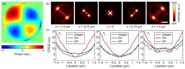
(Color online): (a) Saddle-Point (SP) PSF, optimized for high background, low signal 3D precision over a 3 μm depth range. (b) Calculated PSF for various z positions (stated). Scale bar: 1 μm (in sample space). (c) Calculated CRLB of the SP PSF for x, y, z vs. astigmatic (Astigm.) and DH PSF as a function of z. 3500 detected signal photons per frame and β = 50 were considered. Astigmatic axes are at 45⁰ relative to camera axes, hence the similar x and y behavior.

To experimentally demonstrate localization performance for subwavelength-sized emitters under typical biological fluorescence imaging conditions, we imaged 100 nm diameter fluorescent nanospheres on a standard microscope cover glass, using an inverted NA 1.4 oil immersion microscope system with custom widefield laser excitation and equipped with an EMCCD image sensor. Phase masks were loaded onto an SLM placed in the Fourier plane as described in [13] and schematically shown in Fig. 1. Fluorescence was excited using a 514-nm argon ion laser filtered by a dichroic and band pass filter (578/105). A controllable background level β at the sample was produced by the microscope stand’s white light illuminator [27].

The localization procedure consists of the following steps: First, a set of calibration measurements is taken. A nanosphere is scanned at defined z positions by stepping with an axial objective positioner (Δz = 50 nm), and a calibration dictionary of the PSF at these increments is thus experimentally created. Then, given a measured image of an emitter, localization is performed using a maximum-likelihood estimator (MLE) [25]. The MLE approach is increasingly used in super-resolution single-molecule imaging to estimate an emitter’s position (x,y,z) as well as possibly the number of signal and background photons (a total of 5 parameters), given a measured noisy image frame and an imaging model. MLE finds the set of parameters that yield the best (most likely) correspondence of experimental image and model given the measured data, along with image formation and noise models. We create a continuous image formation model, necessary for the MLE, by using locally phase-retrieved masks calculated from the measured dictionary [31]. See [27] for the detailed estimation method.

Figure 3 shows experimental localization results. After creating a measured dictionary (examples at different z positions in Fig. 3a), a nanosphere was placed in various z positions, and imaged for 500 frames under typical super-resolution conditions (mean detected signal photons per frame was ~3470, and mean background photons per pixel β ≈ 43). Each frame was then localized with MLE, using the locally-phase-retrieved masks, calculated from the dictionary measurements in the 300 nm range surrounding the initial estimate of the emitter position. The standard deviation of the 500 measurements at each z position defines the localization precision.

FIG 3.

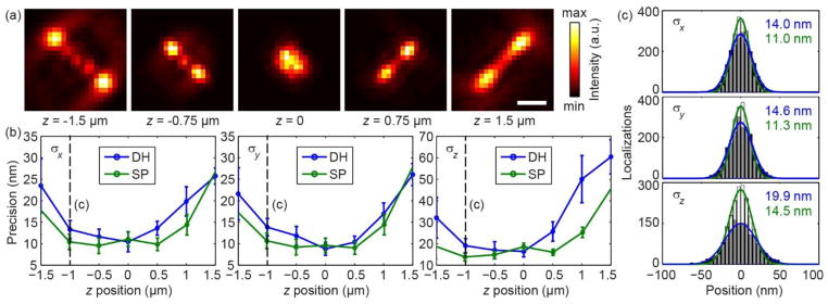
(Color online): (a) Experimental realizations of the Saddle-Point (SP) PSF for various z positions (stated). Scale bar: 1 μm (in sample space). Images were re-scaled to min/max intensity on an individual basis. (b) Experimental measurements of statistical localization precisions as the standard deviations σ_x, σ_y, σ_z of localization outcomes from 500 camera frames. Bars show standard deviations derived from n = 4 independent experiments. (c) Experimental histograms of localization outcomes along the x, y and z dimensions, recorded at z = −1 μm (dotted lines in (b), data from 4 measurements). Extracted σ_x, σ_y, σ_z are stated.

The localization process was repeated using the double-helix mask as well, and the entire measurement procedure was performed on four different nanospheres. The precision results are shown in Fig. 3b. The saddle-point mask exhibits superior performance to the DH-PSF in all three dimensions throughout almost the entire tested 3μm depth range. Figure 3c shows example precision histograms of all 2000 detected positions for both PSFs, at z = −1 μm.

To further demonstrate the generality and one of the new possibilities opened by our method, we use it to optimize a PSF for a challenging very large imaging depth for a single PSF of 6 μm. This is done by minimizing the 3D CRLB with the same parameters as before, but this time over a 6 μm z-range. The resulting mask and its experimental validation are described in [27].

Discussion

While the behavior of the experimentally tested phase masks is qualitatively similar to the theoretical CRLB calculations, there are apparent discrepancies between theory and experiment (comparing Fig. 2c with 3b). This stems from several possibilities, such as noise model mismatch, non-constant background, and variations in actual photon number. However, the most crucial contribution to this discrepancy is imaging model mismatch: The experimentally produced PSF is somewhat different from the computed one (compare Fig. 2b to 3a). This is due to polarization effects, broadband fluorescence detection, and additional aberrations that are unaccounted for in our imaging model. However, the experimental precision matches the CRLB calculated from the experimentally measured dictionary very well (see [27] for this result). This means that the CRLB is not only a mathematical limit, but indeed an experimentally valid criterion for optimization, which yields a measureable performance benefit.

In this work we have demonstrated a new, general method for PSF design that produces information-optimal PSFs subject to system conditions. The optimal PSFs have no prior constraints on their shape. We have applied our method to produce optimal PSFs for 3D high-precision spatial localization over large z-ranges. These PSFs can immediately be used for SPT and SR microscopy; see [27] for an experimental tracking demonstration using our PSF with a 6 μm range. The PSFs can be also used for other applications such as bead location monitoring in magnetic tweezer experiments. The optimization design routine may draw on other sets of basis functions for propagating electromagnetic fields than were used in this first illustration, and may even include aspects of anisotropic dipolar emission [8,26]. In addition to future technical improvements (e.g. brighter emitters, better detectors, etc.), treating the PSF as a free design parameter, as suggested in this Letter, is a powerful way to enhance the performance of a variety of challenging imaging scenarios.

References

- 1.Dupont A, Lamb DC. Nanoscale. 2011;3:4532. doi: 10.1039/c1nr10989h. [DOI] [PubMed] [Google Scholar]
- 2.Thompson MA, Casolari JM, Badieirostami M, Brown PO, Moerner WE. Proc Natl Acad Sci U S A. 2010;107:17864. doi: 10.1073/pnas.1012868107. [DOI] [PMC free article] [PubMed] [Google Scholar]
- 3.Betzig E, Patterson GH, Sougrat R, Lindwasser OW, Olenych S, Bonifacino JS, Davidson MW, Lippincott-Schwartz J, Hess HF. Science. 2006;313:1642. doi: 10.1126/science.1127344. [DOI] [PubMed] [Google Scholar]
- 4.Hess ST, Girirajan TPK, Mason MD. Biophys J. 2006;91:4258. doi: 10.1529/biophysj.106.091116. [DOI] [PMC free article] [PubMed] [Google Scholar]
- 5.Rust MJ, Bates M, Zhuang X. Nat Methods. 2006;3:793. doi: 10.1038/nmeth929. [DOI] [PMC free article] [PubMed] [Google Scholar]
- 6.Small A, Stahlheber S. Nat Methods. 2014;11:267. doi: 10.1038/nmeth.2844. [DOI] [PubMed] [Google Scholar]
- 7.Goodman JW. Introduction to Fourier Optics. Roberts & Company Publishers; Greenwood Village, CO: 2005. [Google Scholar]
- 8.Backer AS, Moerner WE. J Phys Chem B. 2014;118:8313. doi: 10.1021/jp501778z. [DOI] [PMC free article] [PubMed] [Google Scholar]
- 9.Holtzer L, Meckel T, Schmidt T. Appl Phys Lett. 2007;90:053902. [Google Scholar]
- 10.Huang B, Wang W, Bates M, Zhuang X. Science. 2008;319:810. doi: 10.1126/science.1153529. [DOI] [PMC free article] [PubMed] [Google Scholar]
- 11.Piestun R, Schechner YY, Shamir J. J Opt Soc Am A. 2000;17:294. doi: 10.1364/josaa.17.000294. [DOI] [PubMed] [Google Scholar]
- 12.Pavani SRP, Thompson MA, Biteen JS, Lord SJ, Liu N, Twieg RJ, Piestun R, Moerner WE. Proc Natl Acad Sci U S A. 2009;106:2995. doi: 10.1073/pnas.0900245106. [DOI] [PMC free article] [PubMed] [Google Scholar]
- 13.Backlund MP, Lew MD, Backer AS, Sahl SJ, Grover G, Agrawal A, Piestun R, Moerner WE. Proc Natl Acad Sci U S A. 2012;109:19087. doi: 10.1073/pnas.1216687109. [DOI] [PMC free article] [PubMed] [Google Scholar]
- 14.Baddeley D, Cannell MB, Soeller C. Nano Research. 2011;4:589. [Google Scholar]
- 15.Thompson RE, Larson DR, Webb WW. Biophys J. 2002;82:2775. doi: 10.1016/S0006-3495(02)75618-X. [DOI] [PMC free article] [PubMed] [Google Scholar]
- 16.Chao J, Sripad R, Ward ES, Ober RJ. Nat Methods. 2013;10:335. doi: 10.1038/nmeth.2396. [DOI] [PMC free article] [PubMed] [Google Scholar]
- 17.Badieirostami M, Lew MD, Thompson MA, Moerner WE. Appl Phys Lett. 2010;97:161103. doi: 10.1063/1.3499652. [DOI] [PMC free article] [PubMed] [Google Scholar]
- 18.Jia S, Vaughan JC, Zhuang X. Nat Photonics. 2014;8:302. doi: 10.1038/nphoton.2014.13. [DOI] [PMC free article] [PubMed] [Google Scholar]
- 19.Frieden BR. JOSA. 1972;62:511. doi: 10.1364/josa.62.000511. [DOI] [PubMed] [Google Scholar]
- 20.Kay SM. Fundamentals of Statistical Signal Processing: Estimation Theory. Prentice-Hall PTR; Englewood Cliffs, NJ: 1993. [Google Scholar]
- 21.Abraham AV, Ram S, Chao J, Ward ES, Ober RJ. Opt Express. 2009;17:23352. doi: 10.1364/OE.17.023352. [DOI] [PMC free article] [PubMed] [Google Scholar]
- 22.Smith CS, Joseph N, Rieger B, Lidke KA. Nat Methods. 2010;7:373. doi: 10.1038/nmeth.1449. [DOI] [PMC free article] [PubMed] [Google Scholar]
- 23.Mortensen KI, Churchman LS, Spudich JA, Flyvbjerg H. Nat Methods. 2010;7:377. doi: 10.1038/nmeth.1447. [DOI] [PMC free article] [PubMed] [Google Scholar]
- 24.Grover G, DeLuca K, Quirin S, DeLuca J, Piestun R. Opt Express. 2012;20:26681. doi: 10.1364/OE.20.026681. [DOI] [PMC free article] [PubMed] [Google Scholar]
- 25.Ober RJ, Ram S, Ward ES. Biophys J. 2004;86:1185. doi: 10.1016/S0006-3495(04)74193-4. [DOI] [PMC free article] [PubMed] [Google Scholar]
- 26.Backlund MP, Lew MD, Backer AS, Sahl SJ, Moerner WE. ChemPhysChem. 2014;15:587. doi: 10.1002/cphc.201300880. [DOI] [PMC free article] [PubMed] [Google Scholar]
- 27.See Supplemental Material at [URL], which includes Refs. [32–34], for information theoretical aspects, numerical implementation details, experimental methods, tracking results and extended discussion.
- 28.Born M, Wolf E. Principles of Optics. Cambridge University Press; Cambridge: 1999. [Google Scholar]
- 29.Lee HD, Sahl SJ, Lew MD, Moerner WE. Appl Phys Lett. 2012;100:153701. doi: 10.1063/1.3700446. [DOI] [PMC free article] [PubMed] [Google Scholar]
- 30.Huang F, Hartwich TMP, Rivera-Molina FE, Lin Y, Duim WC, Long JJ, Uchil PD, Myers JR, Baird MA, Mothes W, et al. Nat Methods. 2013;10:653. doi: 10.1038/nmeth.2488. [DOI] [PMC free article] [PubMed] [Google Scholar]
- 31.Quirin S, Pavani SRP, Piestun R. Proc Natl Acad Sci U S A. 2012;109:675. doi: 10.1073/pnas.1109011108. [DOI] [PMC free article] [PubMed] [Google Scholar]
- 32.Fienup JR. Opt Lett. 1978;3:27. doi: 10.1364/ol.3.000027. [DOI] [PubMed] [Google Scholar]
- 33.Hanser B, Gustafsson M, Agard D. J Microsc. 2004;216:32. doi: 10.1111/j.0022-2720.2004.01393.x. [DOI] [PubMed] [Google Scholar]
- 34.Mlodzianoski MJ, Juette MF, Beane GL, Bewersdorf J. Opt Express. 2009;17:8264. doi: 10.1364/oe.17.008264. [DOI] [PubMed] [Google Scholar]
Associated Data
This section collects any data citations, data availability statements, or supplementary materials included in this article.