Subject-specific functional parcellation via Prior Based Eigenanatomy

Abstract

We present a new framework for prior-constrained sparse decomposition of matrices derived from the neuroimaging data and apply this method to functional network analysis of a clinically relevant population. Matrix decomposition methods are powerful dimensionality reduction tools that have found widespread use in neuroimaging. However, the unconstrained nature of these totally data-driven techniques makes it difficult to interpret the results in a domain where network-specific hypotheses may exist.

We propose a novel approach, Prior Based Eigenanatomy (p-Eigen), which seeks to identify a data-driven matrix decomposition but at the same time constrains the individual components by spatial anatomical priors (probabilistic ROIs). We formulate our novel solution in terms of prior-constrained ℓ₁ penalized (sparse) principal component analysis. p-Eigen starts with a common functional parcellation for all the subjects and refines it with subject-specific information. This enables modeling of the inter-subject variability in the functional parcel boundaries and allows us to construct subject specific networks with reduced sensitivity to ROI placement.

We show that while still maintaining correspondence across subjects, p-Eigen extracts biologically-relevant and patient-specific functional parcels that facilitate hypothesis-driven network analysis. We construct Default Mode Network (DMN) connectivity graphs using p-Eigen refined ROIs and use them in a classification paradigm. Our results show that the functional connectivity graphs derived from p-Eigen significantly aid classification of Mild Cognitive Impairment (MCI) as well as the prediction of scores in a Delayed Recall memory task when compared to graph metrics derived from 1) standard registration-based seed ROI definitions, 2) totally data driven ROIs 3) a model based on standard demographics plus hippocampal volume as covariates and 4) Ward Clustering based data driven ROIs. In summary, p-Eigen incarnates a new class of prior-constrained dimensionality reduction tools that may improve our understanding of the relationship between MCI and functional connectivity.

1 Introduction & Related Work

The presence of large and diverse neuroimaging datasets has brought the importance of data analysis techniques into focus. These issues are particularly salient in blood oxygen level dependent (BOLD) fMRI where recent papers have highlighted the sensitivity of this modality to specific analysis choices (Carp, 2012; Haller and Bartsch, 2009). Network analysis of functional connectivity within the brain from BOLD data has received a significant amount of attention and is notorious for being sensitive to analysis decisions (Dawson et al., 2012; Eke et al., 2012).

Functional connectivity is defined as the temporal co-activation of neuronal activation patterns between anatomically separated regions of the brain (Aertsen et al., 1989) and is thought to be an indicator of functional communication between these different regions. Typically, functional connectivity studies measure the level of correlation between the time-series of the resting state BOLD signal of the different brain regions (Biswal et al., 1997; Damoiseaux et al., 2006; Salvador et al., 2005). Studying the brain as an integrative network of functionally interacting brain regions can shed new light on large scale neuronal communication in the brain and how this communication is impaired in neurological diseases (Bullmore and Sporns, 2009; Mohammadi et al., 2009; Seeley et al., 2009).

There are two predominant approaches for the analysis of functional connectivity:

• Seed (ROI) Based Approaches: These are straightforward and operate in the traditional confirmatory network paradigm (Tukey, 1977). They involve computing the correlation between the time series of a given (preselected) seed brain region (ROI) ¹ against all the other brain regions, resulting in a set of functional connectivity maps of the given brain regions (Biswal et al., 1997; Cordes et al., 2000). These functional connectivity maps can then be used to construct resting-state-networks of functionally correlated regions in the brain (Fox et al., 2005). The seed region can either be selected based on prior clinical knowledge or it can be selected from the activation map of a separate task dependent fMRI scan.

• Learning Based Approaches: These approaches use statistical techniques to explore functional connectivity in the brain, obviating the need to define a seed region. Typical methods employed are Principal Component Analysis (PCA) (Friston, 1998), Independent Component Analysis (ICA) or its variants e.g. Group ICA (Beckmann and Smith, 2004; Beckmann et al., 2005; Damoiseaux et al., 2006; Varoquaux et al., 2010b; Petrella et al., 2011) or hierarchical methods (Cordes et al., 2002; Salvador et al., 2005; Blumensath et al., 2013). These methods strive to find a set of orthogonal or independent signals in the time series that can explain the resting state activity patterns. ICA based methods are the popular methods in this setting as they can find a set of independent signals from whole brain voxel-wise data and also due to the public availability of tools like MELODIC in FSL (Jenkinson et al., 2012) for ICA and Group ICA of fMRI Toolbox (GIFT) (Calhoun et al., 2001). Subsequently, one can create brain connectivity networks from the outputs of these approaches by computing correlations between the different (independent/orthogonal) signals they find.

The brain networks found by the above approaches are represented as a set of vertices (brain regions) connected by edges which represent the strength of correlation between those two regions (He and Evans, 2010; Stam et al., 2007). Various independent studies (surveyed here (van den Heuvel and Hulshoff Pol, 2010)) have consistently found a set of eight functional connectivity networks in the brain. One can use a set of key properties of the network graph e.g. clustering coefficient, centrality and modularity to get further insights into the flow of neuronal signals within a network (He and Evans, 2010; Stam et al., 2007).

The above mentioned approaches for analyzing functional connectivity and constructing brain networks suffer from a variety of problems. The Group ICA based approaches do a group decomposition of the time series’ images of the entire cohort; they have an averaging effect and erode away any subject specific characteristics of the network. So, the Group ICA analysis is usually followed by a back reconstruction step to generate subject specific functional connectivity maps (Smith et al., 2011). However, it is unclear how to choose a statistically justified threshold to binarize these maps.

The seed based approaches also suffer from the problem of averaging the signal and may be sensitive to ROI placement (Zhang et al., 2012), co-registration errors and the specific ROI boundaries. These approaches assume that the signal lies totally within a predefined region. However, the important signal may have slightly different boundaries than the scientist’s conception. The data representation (or spatially varying noise) may also lead to strong or weak signal within different parts of the ROI. Such dataset specific information is not taken into account by a traditional seed based approach. When effects are localized to the selected region, and that region is well-defined, a seed based analysis may provide the most sensitive testing method. However, some conditions involve a network of regions that may not be fully identified.

Furthermore, it has been shown that decreased/impaired functional connectivity in certain brain networks, for instance, the Default Mode Network (DMN) has association with neurodegenerative disorders e.g. Alzheimer’s Disease (AD) (Greicius et al., 2004; Sheline et al., 2010), schizophrenia (Liu et al., 2008; Whitfield-Gabrieli et al., 2009), multiple sclerosis (MS) (Lowe et al., 2008), mild cognitive impairment (MCI) (Petrella et al., 2011; Agosta et al., 2012; Hedden et al., 2009; Bai et al., 2009). So, it has become even more imperative to improve statistical analysis methods to efficiently leverage the scarce patient BOLD fMRI data that is typically available.

In this paper, we propose a method that integrates ideas from both the seed based and learning based approaches. Our contributions in this paper are three fold.

1. We contribute a general method for prior constrained eigendecomposition (p-Eigen) of high-dimensional matrices and a novel algorithm for its optimization.

2. Publicly available implementation of our approach in C++.

3. Application of p-Eigen for deriving subject specific functional parcellations from BOLD data (which are later used to derive functional networks) and an evaluation of these novel measurements in the context of mild cognitive impairment and prediction of delayed recall in a memory task.

Our approach provides a principled way of incorporating priors in an otherwise totally data driven approach based on Sparse Principal Component Analysis (SPCA) (Zou et al., 2006; Witten et al., 2009; d’Aspremont et al., 2007; Shen and Huang, 2008).

p-Eigen allows an initial binary or probabilistic ROI to adapt to the underlying subject specific covariation within the data. At the same time, p-Eigen maintains proximity to (and the locality of) the original region and thus retains the advantages of the standard seed based approach. p-Eigen also maintains non-negativity in the estimated anatomically-constrained eigenvector, thereby keeping ROI interpretability. This allows us to modify the definitions of labels to capture the variation in dataset (a given subject’s time series) while still staying close to the initial ROI definitions. p-Eigen therefore produces labelings with “soft” weighted averages and as we show in the experimental section, are more sensitive to the underlying brain data than a standard ROI.

Given an ROI set, p-Eigen has only one key parameter to tune- the weight of the prior term guiding the decomposition. Therefore, our optimization objective provides a tradeoff between 1). staying close to the initial ROI definitions and 2). allowing data to lead the exploratory analysis by explaining variance through PCA. A good way to think about this is as ROI definitions forcing us to be conservative and staying close to the initial brain parcellation; on the other hand the SPCA component gives us liberty to be either more exploratory or more focused on the content of the given dataset. The tradeoff between the two competing paradigms is defined by user tunable (prior strength) parameter, which is chosen via cross validation.

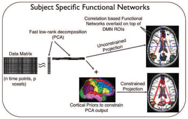
p-Eigen does a prior constrained sparse decomposition of each subject’s time series image separately to create subject specific functional networks, so it does not suffer from the problem of averaging as Group ICA does. Moreover, the priors help us maintain a direct correspondence between the anatomy of the same regions across different subjects hence leading to better clinical interpretability. Our proposed approach is shown in Fig. 1.

Fig. 1.

Prior Based Eigenanatomy (p-Eigen). An initial data matrix (subject’s time series in this case) is decomposed into its eigenvectors, with each eigenvector being constrained by a corresponding cortical prior.

We have drawn a clear contrast between our approach and the two related approaches namely seed based approaches (no influence of data) and Group ICA/PCA based approaches (only data driven). That said, there has also been substantial work on incorporating prior information across subjects to build subject specific functional networks as proposed by this paper.

Some early work that performed PCA on fMRI signal within ROIs (Nieto-Castanon et al., 2003) clearly foreshadowed p-Eigen. (Thirion et al., 2006) also proposed a spectral learning based technique for parcellation that delineates homogeneous and connected regions across subjects, providing subject specific functional networks.

The research that is perhaps closest to ours is (Ng et al., 2009a), (Deligianni et al., 2011) and (Blumensath et al., 2013). (Ng et al., 2009a) used group replicator dynamics (GRD) for finding sparse functional networks that are common across subjects but have subject specific weightings of the brain regions. (Langs et al., 2010) performed functional alignment across subjects to achieve improved functional correspondences across subjects. (Deligianni et al., 2011) used brain anatomical connectivity to constrain the conditional independence structure of functional connectivity via a multivariate autoregressive model. (Blumensath et al., 2013) perform hierarchical parcellation of the brain with a further clustering of the parcels to derive spatially contiguous parcels. Closely related is the work (Ng et al., 2009b) which constrains the PCA output by employing neighborhood information to learn spatially contiguous clusters. Recently, we proposed and successfully applied a variant of p-Eigen called Anatomically Constrained PCA (AC-PCA) to structural (T1-imaging) data of a clinically relevant population (Dhillon et al., 2013).

Our approach is complementary to these set of approaches and proposes a new formulation to derive subject specific functional parcels (and hence connectivity networks) and also the first one to use the networks to derive covariates for MCI and Delayed Recall prediction.

The remainder of the paper is organized as follows; in the next section we provide the details of p-Eigen. In Section 3, we provide experimental results in which we use p-Eigen to graphically describe the default mode network (DMN) connectivity with hippocampus. We further use the DMN connectivity patterns to classify MCI vs controls, and to predict delayed recall in a memory task. We conclude in Section 4.

2 Our Approach

p-Eigen is based on the methods of sparse principal components analysis (SPCA) (Zou et al., 2006; Witten et al., 2009; d’Aspremont et al., 2007; Shen and Huang, 2008) and singular value decomposition (Sill et al., 2011).

2.1 Prior Based Eigenanatomy: p-Eigen

Define a set of n, t × p (rows by columns) matrices ${\{{\mathbf{X}}_{\mathbf{m}}\}}_{\mathbf{m}=\mathbf{1}}^{\mathbf{n}}$ where t is the number of total time points, p is the number of total voxels and each X_m matrix derives from an observed subject’s BOLD fMRI image. Also, assume that we have a prior matrix M (Fig. 2) each of whose k rows corresponds to a separate prior and each of whose p columns contains the probability of a particular voxel belonging to that prior.

Fig. 2.

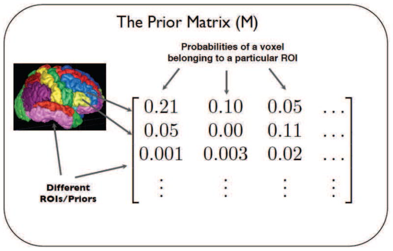
Prior Matrix (M). Each row corresponds to a different ROI (Total k of them) and each column corresponds to a different voxel in the brain (Total p of them).

We seek a sparse decomposition of the X_m matrices constrained by the anatomical priors M which should give us a t × k matrix for each subject where each of the k eigenvectors explains the variance in the corresponding anatomical region specified by the prior.

Our objective is described by Equation 1.

$$v_i^{\ast }=\underset{v_i,\Vert v_i\Vert =1,v_i^{\top }{v}_j=0,i\ne j,v_i\succcurlyeq 0}{\text{argmax}}{v_i}^{\top }\left(\mathbf{C}+\theta ·m_i^{\top }{m}_i\right)v_i-{\lambda }_i{\Vert v_i\Vert }_1^{+}$$ (1)

where m_i is the i^th prior and is itself a vector of size (1 × p). C is the covariance matrix X^⊤X. θ is a user tunable parameter which controls the tradeoff between the influence of data and the prior and should be typically tuned on a held out validation set in the absence of other knowledge. Smaller values of θ suggest that we trust data more and as θ is increased the eigenvectors v are increasingly influenced by the prior. The ${\Vert v_i\Vert }_1^{+}$ term ensures sparsity and non-negativity in the eigenvectors; in addition to this we enforce unit norm and orthogonality constraints on sparse eigenvectors.

2.1.0.1 Connection to Sparse PCA

Our objective (Equation 1) is intimately connected to the variance maximization formulation of sparse principal components analysis (SPCA) (Zou et al., 2006; Witten et al., 2009) :

$$v_i^{\ast }=\underset{v_i,\Vert v_i\Vert =1,v_i^{\top }{v}_j=0,i\ne j}{\text{argmax}}{v_i}^{\top }\mathbf{C}{v}_i-{\lambda }_i\Vert v_i{\Vert }_1$$ (2)

where terms have the same meaning as in Equation 1.

As can be seen, our objective entails that instead of finding the eigenvectors of the data covariance matrix as done by SPCA, we find the eigenvectors of the transformed data covariance matrix obtained by “regularizing” it by the prior information. An important consequence of this is that we are not confining our data driven priors to lie in the original ROIs but rather we are encouraging them to find ways to explain data variance in this new “prior regularized” space.

One could optimize the p-Eigen objective in Equation 1 using an iterative approach like power iteration. However, in our experience we found the standard power iteration to be unstable and got more efficient and stable solutions using an optimization approach which performs iterative soft-thresholding on the conjugate gradient of the Rayleigh Quotient. In addition, we deflate our data matrix X (factoring out the effect of other eigenvectors) between computations of different eigenvectors, which lead to better solutions (Mackey, 2008). The resulting method is related to the Non-linear Iterative Partial Least Squares (NIPALS) algorithm (Wold et al., 1987) for large scale PCA which also combines deflation with estimation of the principal eigenvector.

2.2 An Algorithm for p-Eigen

In this section we provide an alternating optimization approach, also called an analysis-synthesis loop (Murphy, 2012) for solving the p-Eigen optimization problem. As was briefly mentioned at the end of the last section, our optimization performs iterative soft-thresholding on the conjugate gradient of the Rayleigh Quotient and further relies on deflation to get better quality solutions.

Iterative soft-thresholding (soft(a, δ) ≜ sign(a)(||a||−δ)₊ with x₊ =max(x,0)) falls in the class of proximal gradient methods and has been shown to have better convergence (Bredies and Lorenz, 2008) and scalability properties compared to other sparse optimization algorithms e.g. Least Angle Regression (LARS) (Yang et al., 2010). Furthermore, deflation has been shown to give better sparse PCA solutions (Mackey, 2008); so we added a deflation step between the alternating optimizations.

The deflation based optimization of Equation 1 entails performing an additional ordinary least squares regression (OLS) step and can be motivated as follows.

We know that the best rank ‘k’ reconstruction of a matrix i.e. argmin_X̂ ||X − X̂||², is provided by its first ‘k’ eigenvectors (Eckart and Young, 1936) i.e. $\widehat{\mathbf{X}}={\sum }_{i=1}^k{d}_k{u}_k{v}_k^{\top }$.

Hence, the best rank-1 approximation of X, i.e. the n × 1 and p × 1 vectors ũ, ṽ such that,

$${\stackrel{\sim }{u}}^{\ast },{\stackrel{\sim }{v}}^{\ast }={\mathit{min}}_{\stackrel{\sim }{u},\stackrel{\sim }{v}}{\Vert \mathbf{X}-\stackrel{\sim }{u}{\stackrel{\sim }{v}}^{\top }\Vert }^2$$ (3)

is given by the SVD solution– ũ = u₁ and ṽ = d₁v₁, where u₁, v₁ and d₁ are the first left and right eigenvectors and the eigenvalue, respectively, of the X matrix.

Proceeding this way, $d_2{u}_2{v}_2^{\top }$ provide the best rank-1 approximation of the “deflated” matrix $\mathbf{X}-d_1{u}_1{v}_1^{\top }$ and so on.

As pointed by (Shen and Huang, 2008), with ṽ fixed, the above optimization over ũ is equivalent to a least squares regression of X on ṽ.

Similarly, with ũ fixed, the optimization over ṽ is a sparse optimization problem. As mentioned in the last section, we solve this by iterative soft thresholding on the conjugate gradient of Rayleigh Quotient.

So, our implementation alternates between the optimization of Equations 4, 5 (shown below for iteration number ‘s’) till convergence.

$${{\mathbf{U}}^{\ast }}_s=\underset{U,\Vert U\Vert =1,u_i^{\top }{u}_j=0,i\ne j}{\text{argmin}}{\Vert \mathbf{X}-{\mathbf{UV}}_{s-1}^{\top }\Vert }^2$$ (4)

$${\{v_i^{\ast }\}}_s=\underset{v_i,\Vert v_i\Vert =1,v_i^{\top }{v}_j=0,i\ne j,v_i\succcurlyeq 0}{\text{argmax}}{v_i}^{\top }\left({\mathbf{C}}_s^{\backslash i}+\theta ·m_i^{\top }{m}_i\right)v_i-{\lambda }_i{\Vert v_i\Vert }_1^{+}$$ (5)

where symbols have the same meaning as in Equation 1. ${\mathbf{C}}_s^{\backslash i}$ is the covariance matrix created from the “deflated” X matrix. ${\mathbf{C}}_s^{\backslash i}\triangleq {\mathbf{X}}_{\backslash \mathbf{i}}^{\top }{\mathbf{X}}_{\backslash \mathbf{i}}$ where ${\mathbf{X}}_{\backslash i}\triangleq \mathbf{X}-{\sum }_{j=1,j\ne i}^k{u}_j^{(s)}{v}_j^{\top (s-1)}$.

The sparseness is enforced by a soft-thresholding algorithm as in (Zou et al., 2006; Witten et al., 2009). We denote this function as S(v, λ) and choose λ in a data driven way as ${\lambda }_i={\sum }_{j=1}^p\frac{m_{ij}}{p}$. In other words, we are constraining the sparsity of our eigenvectors to be equal to the weighted size of the corresponding prior ROI. Defining sparsity in this manner via neuro-anatomical priors has biological motivation, as the sizes of ROIs are approximately equal to the sizes of different areas of the brain that we are modelling.

In addition to the sparsity penalty, we also include an optional minimum cluster size threshold, as is commonly performed in Voxel Based Morphometry (VBM)-type analyses. We have found that including a minimum cluster threshold size generally improves robustness of results by getting rid of isolated voxels and also helps prevent overfitting. In the experiments presented in this paper, we chose the minimum cluster threshold as 100 voxels.

Similar to (Zass and Shashua, 2006; Hoyer, 2002), non-negativity in the eigenvectors is enforced by repeated projection onto the feasible (non-negative) set. In between different iterations of our algorithm, the negative values in the eigenvectors are zeroed and the optimization is continued.

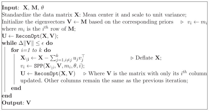
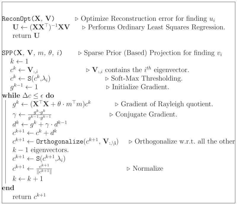
The details of our algorithm can be found in Algorithms 1, 2. Note that the OLS regression step is just required to compute u which is required for deflation of the data matrix.

Algorithm 1.

Prior Based Eigenanatomy: p-Eigen (Main Algorithm)

3 Experiments

In this section we show the performance of p-Eigen on resting-state BOLD fMRI data. We use subject specific functional parcellations generated by p-Eigen to construct subject specific functional connectivity networks.

Algorithm 2.

Prior Based Eigenanatomy: p-Eigen (Sub Algorithm)

Our data consists of time series images of 59 individuals (28 females and 31 males) with 34 controls and 25 subjects diagnosed clinically with Mild Cognitive Impairment (MCI). Patients were diagnosed according to the criterion of Petersen (2004). The memory measure used to get the delayed recall score was the Consortium to Establish a Registry for Alzheimer’s Disease (CERAD) Word List Memory (WLM) test (Morris et al., 1989). Each time series had a total of 120 points. The basic statistics for the cohort are given in Table 1.

Table 1.

Basic statistics for the cohort.

Characteristic	Entire Cohort (μ ± σ)	Only Controls (μ ± σ)	Only Patients (μ ± σ)
Age	70.4 ± 8.5	69.9 ± 9.4	71.1 ± 7.0
Education	16.7 ± 2.7	16.4 ± 3.0	17.2 ± 2.3
Delayed Recall	6.2 ± 3.2	8.4 ± 1.6	3.1 ± 1.8
Total Hippocampal Vol.	4065.2 ± 766.8	4281.7 ± 642.0	3770.8 ± 835.0

Images were acquired on a 3T Siemens Trio scanner. The imaging protocol included the following sequences: 1 mm³ T1-weighted structural MRI and 3×3×3 mm³ resting-state BOLD fMRI covering the entire brain (TR/TE = 4000/30 ms; Matrix = 64×64; 40 axial slices).

3.1 Data Preprocessing

We used ANTs (Avants et al., 2009) to preprocess the data and used a subset of the AAL labels (80 cortical labels out of the total 116 labels) as our seed ROIs (Tzourio-Mazoyer et al., 2002). The list of 80 cortical labels is in Appendix A. Firstly, we registered the AAL labels which were in template space to subject T1 space and then subsequently registered them to the BOLD space. Once in BOLD space, we multiplied the labels with a gray matter probability mask to smooth the labels and convert them to probabilities as well as to reject labelings in non-cortical regions.

We embrace a minimalistic approach to resting-state fMRI processing that seeks to use widely accepted methods to factor out nuisance variables within subject-space (Glasser et al., 2013). The first step in our process involves motion correcting each time-slice of the BOLD image to the average BOLD image in order to capture motion parameters. The first five time slices are discarded before further processing. We then identify physiological noise with the Com-pCor algorithm (Behzadi et al., 2007). Motion and CompCor parameters are then residualized off of the time series matrix. Subsequently, we apply a band pass filter to the time-series data with lower and upper frequencies of 0.01 and 0.1 respectively. No spatial smoothing is performed and all computations are undertaken within the original subject’s BOLD space.

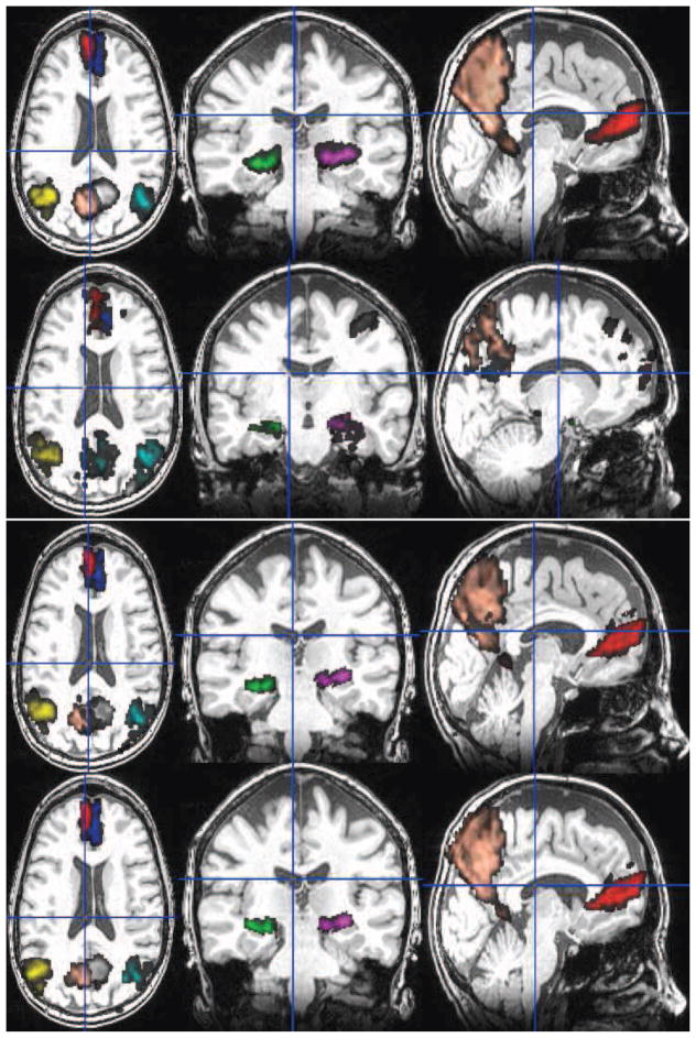
After subject-specific preprocessing, we used p-Eigen to create the constrained eigenvectors ${\{{\mathbf{v}}_{\mathbf{i}}\}}_{\mathbf{i}=\mathbf{1}}^{\mathbf{k}}$. Once we had the eigenvectors, we used a total of eight labels for our study on the default mode and hippocampus network. The eight AAL ROIs that we used along with their modified counterparts after running p-Eigen are shown in Figures 4, 5, 6, 7, 8.

Fig. 4.

Row 1: The original 8 AAL ROIs; Row 2: PCA modified ROIs; Row 3: p-Eigen modified ROIs (θ = 0.5); Row 4: p-Eigen modified ROIs (θ = 0.80) for a randomly chosen subject. 6 of these 8 ROIs are from the default mode network (Precuneus (L/R), Angular Gyrus (L/R), Frontal Medial Orbital Lobe (L/R)) and the remaining two are from left and right parts of hippocampus.

Fig. 5.

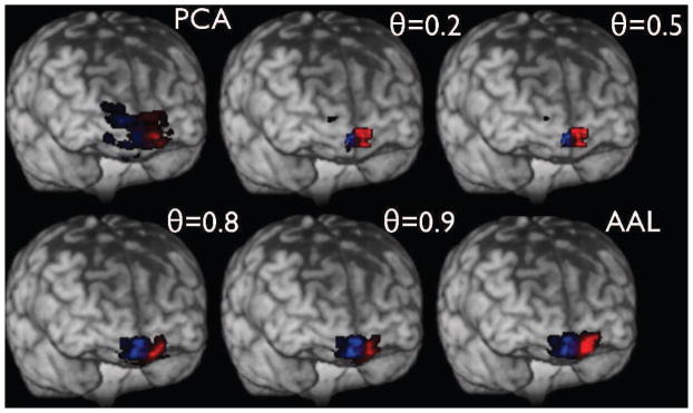
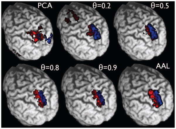
Modified Frontal Medial Orbital Lobe ROIs as a function of θ for a randomly chosen subject.

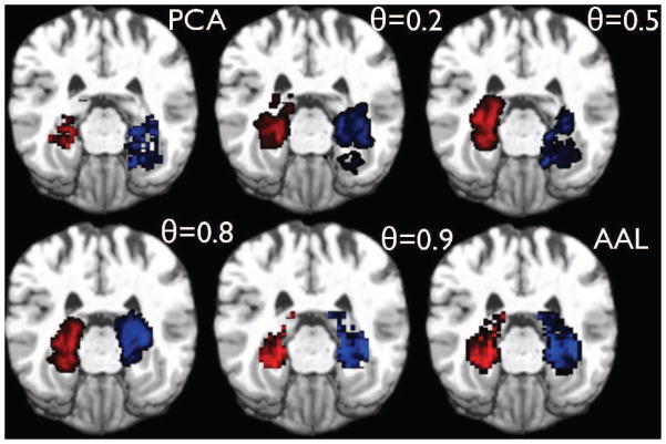
Fig. 6.

Modified Hippocampal ROIs as a function of θ for a randomly chosen subject.

Fig. 7.

Modified Angular Gyrus ROIs as a function of θ for a randomly chosen subject.

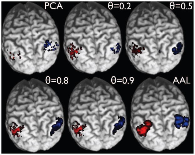
Fig. 8.

Modified Precuneus ROIs as a function of θ for a randomly chosen subject.

It is worth clarifying that since the algorithms for PCA and p-Eigen optimization are iterative in nature, they need an initialization of eigenvectors. In order to make a fair comparison we initialize the eigenvectors with the AAL ROIs both for PCA as well as p-Eigen. We did not have to initialize them this way for PCA, as it is oblivious to any prior information, and has no correspondence between the eigenvectors and the ROIs; however we did that just in order to make a fair comparison. In the case of PCA the eigenvectors drift away freely whereas for p-Eigen they remain close to the priors based on the strength of the prior weight.

Next, we computed the regularized partial correlations between the mean BOLD signal across all the 120 time series points, which were used to construct the functional connectivity graphs for all the three methods AAL, PCA and p-Eigen.

Regularized partial correlations have been shown to be a more robust measure of graph connectivity than simple correlations or partial correlations (Smith et al., 2011; Varoquaux et al., 2010a). We estimated them using Graphical Lasso, which also imposes sparseness on the estimated partial correlations, making the derived network more interpretable (Friedman et al., 2008).

Note that we run p-Eigen and find partial correlations using all the 80 cortical ROIs in order to explain the covariation in the entire cortex. Finally, we derive covariates for MCI classification and delayed recall prediction from only the eight nodes in the default mode and hippocampus network post hoc due to their strong association with MCI as has been pointed out by (Petrella et al., 2011; Agosta et al., 2012; Hedden et al., 2009; Bai et al., 2009).

3.2 Choosing tunable parameters

We used the Graphical Lasso R package (Friedman et al., 2008) for estimating regularized partial correlations and the GLMNET R package (Friedman et al., 2009) for Elastic Net classification.

The Graphical Lasso has a tunable parameter (hyperparameter) ρ which controls the amount of regularization (sparsity in the estimated regularized partial correlations), with ρ = 0 corresponding to no regularization. Further, the Elastic Net has two tunable parameter α and β. α controls the sharing of strength between ℓ₂ and ℓ₁ penalties with a smaller α corresponding to a bigger ℓ₂ regularization. β scales the strength of the penalty terms (ℓ₂ and ℓ₁) relative to the data term, just as in any penalized regression. In addition to this, p-Eigen has a tunable parameter θ which controls the effect of the priors, with higher values corresponding to larger effect of prior.

We tuned all these parameters in a totally data driven manner via a nested leave 5 out cross validation (CV), where we tried values of ρ, α ∈ [0,1] in steps of 0.02, β ∈ [0,2] in steps of 0.05 and ρ ∈ [0.05, 0.95] in steps of 0.1. In order to be totally objective and be completely fair to all the methods, we tuned these parameters separately for all the three methods AAL, PCA and p-Eigen for the tasks of MCI vs. Normal classification and prediction of Delayed Recall in a memory task. Finally, we choose the parameters corresponding to the minimum CV error.

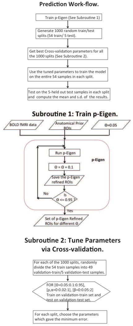
The work-flow showing the details of our approach is shown in Figure 3.

Fig. 3.

Work-flow showing our prediction pipeline.

The results reported in the next subsection use the “best” values of these tunable parameters that we found in the cross validation (CV) and are reported in the Table 2.

Table 2.

Best values (minimum CV error on most validation splits) of the tunable parameters chosen via CV. Parameters for Delayed Recall for Patients in parenthesis. Note that the implicit value of θ for AAL is 1 and for PCA is 0.

	MCI vs Control			Delayed Recall (Patients)
Parameter	p-Eigen	AAL	PCA	p-Eigen	AAL	PCA
ρ	0.2	0.26	0.66	0.74 (0.64)	0.88 (0.58)	0.88 (0.4)
α	0.94	0.44	0.08	0.02 (0.48)	0.02 (0.72)	0.02(0.36)
β	0.1	2	0.1	1.7 (0.4)	0.7 (1.7)	0.7 (0.9)
θ	0.80	N/A	N/A	0.80	N/A	N/A

3.3 Results

We used our functional connectivity graph network information for classifying controls vs MCI. We also used the network information to predict the Delayed Recall for the entire cohort as well as for the patients.

In all the experiments reported below, we perform a leave-5-out cross validation (separate from the one used to tune the hyperparameters) i.e. training on 54 and testing on 5, and this procedure was repeated a 1000 times. We used an Elastic Net classifier whose parameters were tuned as described earlier.

The base features that we used in our classification tasks were, age, education, gender and Hippocampal Volume (Total left and right, as well as separately for left and right hemisphere) of the subject. As described earlier, in addition to this, we used the sparse inverse correlation matrix of the DMN network (which was estimated using Graphical Lasso) as features.

The results are summarized in the Tables 3 and 4.

Table 3.

Results showing p-Eigen better than just using the Base Features. For MCI vs. Normal we report mean classification error (e.g. 0.24 ↝ 24%), whereas for Delayed Recall we report Mean Absolute Prediction Error ( ${\sum }_{i=1}^n\frac{\Vert y_i-{\widehat{y}}_i\Vert }{n}$). The p-values from two sample t-tests for all columns are 2.2 × 10⁻¹⁶.

Feature Set	MCI vs. Normal (μ ± σ)	Delayed Recall (All) (μ ± σ)	Delayed Recall (Patients) (μ ± σ)
Base Features	0.42 ± 0.08	2.68 ± 0.35	1.47 ± 0.30
+ p-Eigen	0.24 ± 0.06	1.83 ± 0.29	0.97 ± 0.18

Table 4.

Results showing p-Eigen better than AAL and PCA ROI labels. For MCI vs. Normal we report mean classification error (e.g. 0.24 ↝ 24%), whereas for Delayed Recall we report Mean Absolute Prediction Error ( ${\sum }_{i=1}^n\frac{\Vert y_i-{\widehat{y}}_i\Vert }{n}$). All the classifiers also used Base Features in addition to the graph measurement features from ROIs. The p-values from two sample t-test for p-Eigen vs AAL and PCA are 2.2 × 10⁻¹⁶.

#	FeatureSet	MCI vs. Normal (μ ± σ)	Delayed Recall (All) (μ ± σ)	Delayed Recall (Patients) (μ ± σ)
1.	AAL	0.36± 0.05	2.34 ± 0.21	1.41 ± 0.28
2.	PCA	0.34± 0.06	2.41 ± 0.35	1.35 ± 0.21
3.	p-Eigen	0.24± 0.06	1.83 ± 0.29	0.97 ± 0.18

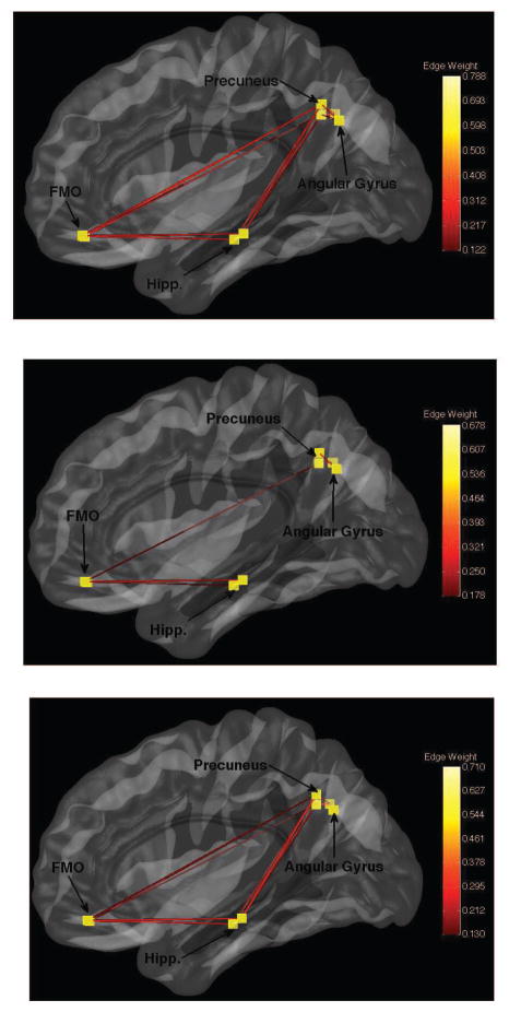
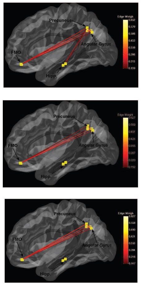
The obtained networks for the AAL, PCA and p-Eigen labels are shown in Figures 11, 13 and the corresponding heatmaps are show in Figures 12 and 14.

Fig. 11.

Default Mode Networks for a randomly chosen control. Top-to-Bottom AAL, PCA, pEigen. Key: FMO-Frontal Medial Orbital.

Fig. 13.

Default Mode Networks for a randomly chosen patient. Top-to-Bottom AAL, PCA, pEigen. Key: FMO-Frontal Medial Orbital.

Fig. 12.

Heatmaps for brain networks connectivity for the same randomly chosen control as above. AAL, PCA, pEigen (L-to-R). Key: FMO-Frontal Medial Orbital, AG-Angular Gyrus, P-Precuneus, Hipp.-Hippocampus.

Fig. 14.

Heatmaps for brain networks connectivity for the same randomly chosen patient as above. AAL, PCA, pEigen (L-to-R). Key: FMO-Frontal Medial Orbital, AG-Angular Gyrus, P-Precuneus, Hipp.-Hippocampus.

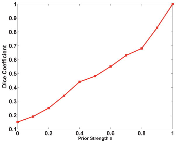
The Dice coefficient for p-Eigen as a function of the prior strength parameter θ is shown in Figure 9. A prior strength of zero corresponds to totally data driven (PCA) based decomposition and a prior strength of one corresponds to using only the prior. As expected, there is increasing overlap between the p-Eigen refined ROIs and the true AAL ROIs as the prior strength increases.

Fig. 9.

Dice coefficient for p-Eigen for the randomly chosen subject (same as Figure 4) with AAL ROIs as a function of the prior strength parameter θ. The plotted dice coefficient ( $=2\frac{\mid A\cap B\mid }{\mid A\mid +\mid B\mid }$, where A is the p-Eigen modified ROI and B is the true AAL ROI ) was computed as the average of dice coefficients over all the 8 DMN ROIs.

Our main findings are:

1. p-Eigen network measurements along with the base features are a significantly better predictor of both MCI status and Delayed Recall score compared to using the base features alone.

2. p-Eigen network measurements along with the base features are a significantly better predictor of both MCI status and Delayed Recall score compared to using AAL or PCA ROI graph measurements along with the base features.

3.4 Robustness of p-Eigen

In this section we first show some additional experiments which highlight the robustness of our approach. Particularly, we consider alternate definitions of initial ROIs and the use of other measures of correlation to construct networks.

Sensitivity to the Choice of ROIs

To investigate the sensitivity of our results we considered an alternative ROI set constructed using Ward Clustering (Michel et al., 2012). We parcellated the average time-series image of the subjects using Ward Clustering (we used the implementation from NILEARN (http://nilearn.github.io/)) with 80 clusters and then used those as the prior ROIs for p-Eigen. The corresponding method is called p-Eigen (Ward).

In addition, we also compared p-Eigen against another baseline. We created subject specific parcellations by intersecting AAL ROI labels with the subject specific ROIs obtained by performing Ward Clustering on each subject’s time series image separately and keeping only those clusters that were larger than 100 voxels. This provides a simple baseline method to construct subject specific parcellations and hence functional connectivity networks.

The results are shown in Table 5 and the corresponding intersected ROIs are shown in Figure 10. We can make two observations from the results. Firstly, p-Eigen with AAL ROIs is statistically significantly better than subject specific parcellations constructed by intersecting AAL labels with Ward clusters. This shows that subject specific functional parcellations constructed using p-Eigen contain more discriminative signal to aid MCI and delayed recall prediction.

Table 5.

Results comparing 1). p-Eigen with Ward Clustering based ROIs and 2). p-Eigen with AAL ROIs vs p-Eigen with Ward Clustering based ROIs. For MCI vs. Normal we report mean classification error (e.g. 0.24 ↝ 24%), whereas for Delayed Recall we report Mean Absolute Prediction Error ( ${\sum }_{i=1}^n\frac{\Vert y_i-{\widehat{y}}_i\Vert }{n}$). All the classifiers also used Base Features in addition to the graph measurement features from ROIs. Note: The reported p-values are from a two sample t-test.

#	FeatureSet	MCI vs. Normal (μ ± σ)	Delayed Recall (All) (μ ± σ)	Delayed Recall (Patients) (μ ± σ)
1.	Ward Clustering	0.33 ± 0.08	2.24 ± 0.23	1.21 ± 0.24
2.	p-Eigen (Ward)	0.28 ± 0.05	2.07 ± 0.26	1.10 ± 0.22
3.	p-Eigen (AAL)	0.24 ± 0.06	1.83 ± 0.29	0.97 ± 0.18
	p-value	(2. vs 3.) 0.045 (1. vs 3.) 2.7 × 10−6	(2. vs 3.) 0.041 (1. vs 3.) 1.4 × 10−7	(2. vs. 3) 0.066 (1. vs. 3) 3.4 × 10−5

Fig. 10.

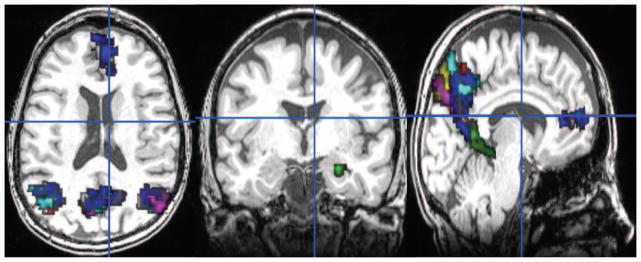
Figure showing only those Ward ROIs that had a non-zero intersection with any of the 8 AAL ROIs and were larger than 100 voxels. There were a total of 7 such ROIs.

Secondly, p-Eigen with AAL ROIs is significantly better (though marginally) than p-Eigen using Ward Clustered ROIs. We conjecture that it is due to the Ward Clustered ROIs being noisy as can be seen in Fig. 10. When we further smoothed them and used them to constrain p-Eigen (p-Eigen (Ward)), the difference was no longer significant.

So, p-Eigen is reasonably robust to the choice of ROIs used for priors, unless they are very noisy. In such cases, smoothing might improve performance.

Using Pearson’s Correlation for Constructing Networks

As mentioned earlier, regularized partial correlations have been shown to be a robust measure of graph connectivity. However, its estimation procedure via Graphical Lasso has a tunable parameter ρ, which needs to be chosen via cross validation. So, we were interested in knowing if we can obviate the need for it by constructing the functional connectivity network using Pearson’s correlation which has no tunable parameters.

The results are shown in Table 6. As can be seen p-Eigen with graph constructed using Graphical Lasso performs significantly better than p-Eigen with the graph constructed using Pearson’s correlation. This can be due to the fact that since regularized partial correlations explain away the effect of all the other nodes in the network while computing correlation between a pair of nodes, they are more robust. Our finding is also in consonance with the finding by (Smith et al., 2011).

Table 6.

Results showing p-Eigen (AAL) with Graphical Lasso better than p-Eigen using Pearson’s correlation. For MCI vs. Normal we report mean classification error (e.g. 0.24 ↝ 24%), whereas for Delayed Recall we report Mean Absolute Prediction Error ( ${\sum }_{i=1}^n\frac{\Vert y_i-{\widehat{y}}_i\Vert }{n}$). All the classifiers also used Base Features in addition to the graph measurement features from ROIs. All other p-values for each column were 2.2 × 10⁻¹⁶.

#	FeatureSet	MCI vs. Normal (μ ± σ)	Delayed Recall (All) (μ ± σ)	Delayed Recall (Patients) (μ ± σ)
1.	AAL (Pearson)	0.39 ± 0.05	2.51 ± 0.23	1.57 ± 0.28
2.	PCA (Pearson)	0.38 ± 0.06	2.59 ± 0.37	1.46 ± 0.21
3.	p-Eigen (Pearson)	0.31 ± 0.04	2.09 ± 0.31	1.11 ± 0.11
4.	p-Eigen (GLasso)	0.24 ± 0.06	1.83 ± 0.29	0.97 ± 0.18
	p-value	(3. vs 4.) 1.3 × 10−4	(3. vs 4.) 2.1 × 10−3	(3. vs. 4) 3.3 × 10−4

4 Discussion

We proposed a new approach for deriving data-driven subject specific functional parcellations. The strong and robust empirical performance of p-Eigen makes it a viable alternative to the seed based or totally data driven approaches. p-Eigen also enhances the findings of several MCI clinical studies.

Multiple clinical studies have reported that there is change in connectivity in default mode network (DMN) for MCI patients as well as for the patients who progress onto clinical Alzheimer’s Disease (AD) (Greicius et al., 2004; Sheline et al., 2010; Petrella et al., 2011; Agosta et al., 2012; Hedden et al., 2009; Bai et al., 2009; He and Evans, 2010).

There are variations in ROI definitions across these studies and furthermore there are some variations on the ROIs thought to be the primary nodes. In this paper, we tried to choose the ROIs corresponding to one of the most widely accepted definitions of DMN. However, differences in definition of the primary nodes of the network maybe a source of some variation across the studies. Nonetheless, there are two consistent and general findings across most MCI studies.

• There is reduced mean connectivity across all the nodes in the DMN for the MCI patients compared to the healthy controls.

• There is reduced mean connectivity of the hippocampus with the other nodes of the DMN (Frontal Medial Orbital, Angular Gyrus, Precuneus in our case) for the MCI patients compared to the healthy controls.

The networks and heatmaps generated by our approach (Figures 11, 13, 12 and 14) for a randomly chosen patient and control illustrate these findings.

First, all the three approaches (AAL, PCA, p-Eigen) highlight that there is reduced mean DMN connectivity in the networks of MCI patients compared to the controls. However, this reduction (averaged over all the subjects) is only significant (p ≈ 0.03 in Welch’s t-test) for p-Eigen ROIs. The corresponding p-values for AAL and PCA are 0.09 and 0.11 respectively.

Second, the memory network is disrupted in patients; they have limited or no connectivity of hippocampus with the DMN. This contrast is more evident in the case of p-Eigen ROIs as the Hippocampus has strong connections to DMN on average for the controls but is not connected (or is weakly connected) to the nodes of the DMN for the patients. In the case of AAL, the Hippocampus also has strong connections to DMN for the controls but the change is less drastic when we compare to patients as some patients also have significant hippocampus connectivity to DMN. Lastly, in the case of PCA, there is no hippocampus connectivity with DMN in the case of patients, but the same is true for controls also, as the PCA networks have very few connections, in general.

A quantitative evaluation of mean connectivity of hippocampus with the nodes of the DMN, shows that the reduction in mean connectivity between controls and patients is highly significant (p < 0.01) for p-Eigen. For AAL and PCA it is again insignificant, however, with a trend towards statistical significance.

We conjecture that it is due to the ability of p-Eigen ROIs to highlight these differences (which have also been confirmed by multiple studies) between controls and patients, that it does a better job of MCI vs. Control classification and Delayed Recall prediction compared to AAL and PCA.

4.1 Limitations

In summary, we showed that p-Eigen better resolves subtle functional patterns that separate MCI from controls and that this is largely consistent with past research. It is also possible that changes in DMN may predict those who convert from MCI to AD and those who do not. While we cannot address this question, it is possible that our MCI data contains subjects of both types. Although this is a limitation in this study, it leads to the possibility that p-Eigen may be extracting signal that is relevant to separating those who do from those who do not progress to AD. This will be a topic of future research. A second limitation of our research is that we explored only a single parcellation scheme, i.e. the AAL. While other parcellation schemes e.g. (Klein and Tourville, 2011; Yeo et al., 2011) may reveal different results, our focus on the relatively consistently defined DMN mitigates this possibility. We did show results which used data-driven Ward Clustering based parcellations and showed that p-Eigen is reasonably robust to the definition of ROIs. However, we think that this needs to be explored more as connectome analyses are known to be sensitive to functional homogeneity (Zuo et al., 2013). We also note that a full exploration of the parameter space of fMRI pre-processing decisions may alter the results reported here. For instance, though we perform motion correction but there might be some residual motion effects in the signal that could affect our results (Van Dijk et al., 2012; Power et al., 2012). We chose a minimal pre-processing pipeline with reasonable control for motion and other nuisance parameters widely recognized as problematic. The fact that we employ a prediction framework and consistent processing across all algorithms compared also mitigates this limitation, although it remains considerable. Finally, we note that we explored only one out of the many possible applications of p-Eigen. Additional work in structural imaging and structural-functional decomposition will be considered in the future.

5 Conclusion

We proposed a novel approach, Prior Based Eigenanatomy (p-Eigen), for fMRI network analysis which integrates ideas from the matrix decomposition and the ROI paradigms. p-Eigen leads to statistically refined definitions of ROIs based on local covariance structure of the data matrix and provides a principled way of incorporating prior information in the form of probabilistic or binary ROIs while still allowing the data to softly modify the original ROI definitions.

The subject specific parcellations generated by p-Eigen were used to construct subject specific functional connectivity networks. These networks showed reduced sensitivity to ROI placement for a cohort of subjects which included people diagnosed with MCI. The network measures gathered from our refined ROIs significantly aid classification of early Mild Cognitive Impairment (MCI) as well as the prediction of Delayed Recall in a memory task when compared to metrics derived from standard registration-based ROI definitions, totally data driven methods, a model based on standard demographics plus hippocampal volume and state-of-the-art Ward Clustering parcellations. We show that the use of our methodology enhances the detection of previously demonstrated findings in this population, namely that there is reduced mean connectivity and disruption of the connections of hippocampus with DMN for MCI patients.

Highlights.

• A novel method for prior constrained decomposition of high-dimensional matrices.

• A novel algorithm for its mathematical optimization.

• Publicly available implementation of our approach in C++.

• Application of our approach to improve network extraction from BOLD data.

• Evaluation on mild cognitive impairment and delayed recall prediction tasks.

A List of 80 AAL (Cortical) ROIs used

The list of 80 cortical ROIs is below.

• 1,Precentral_R

• 2,Precentral_L

• 3,Frontal_Sup_R

• 4,Frontal_Sup_L

• 5,Frontal_Sup_Orb_R

• 6,Frontal_Sup_Orb_L

• 7,Frontal_Mid_R

• 8,Frontal_Mid_L

• 9,Frontal_Mid_Orb_R

• 10,Frontal_Mid_Orb_L

• 11,Frontal_Inf_Oper_R

• 12,Frontal_Inf_Oper_L

• 13,Frontal_Inf_Tri_R

• 14,Frontal_Inf_Tri_L

• 15,Frontal_Inf_Orb_R

• 16,Frontal_Inf_Orb_L

• 17,Rolandic_Oper_R

• 18,Rolandic_Oper_L

• 19,Supp_Motor_Area_R

• 20,Supp_Motor_Area_L

• 21,Olfactory_R

• 22,Olfactory_L

• 23,Frontal_Sup_Medial_R

• 24,Frontal_Sup_Medial_L

• 25,Frontal_Med_Orb_R

• 26,Frontal_Med_Orb_L

• 27,Rectus_R

• 28,Rectus_L

• 29,Insula_R

• 30,Insula_L

• 31,Cingulum_Ant_R

• 32,Cingulum_Ant_L

• 33,Cingulum_Mid_R

• 34,Cingulum_Mid_L

• 35,Cingulum_Post_R

• 36,Cingulum_Post_L

• 37,Hippocampus_R

• 38,Hippocampus_L

• 39,ParaHippocampal_R

• 40,ParaHippocampal_L

• 41,Amygdala_R

• 42,Amygdala_L

• 43,Calcarine_R

• 44,Calcarine_L

• 45,Cuneus_R

• 46,Cuneus_L

• 47,Lingual_R

• 48,Lingual_L

• 49,Occipital_Sup_R

• 50,Occipital_Sup_L

• 51,Occipital_Mid_R

• 52,Occipital_Mid_L

• 53,Occipital_Inf_R

• 54,Occipital_Inf_L

• 55,Fusiform_R

• 56,Fusiform_L

• 57,Postcentral_R

• 58,Postcentral_L

• 59,Parietal_Sup_R

• 60,Parietal_Sup_L

• 61,Parietal_Inf_R

• 62,Parietal_Inf_L

• 63,SupraMarginal_R

• 64,SupraMarginal_L

• 65,Angular_R

• 66,Angular_L

• 67,Precuneus_R

• 68,Precuneus_L

• 69,Heschl_R

• 70,Heschl_L

• 71,Temporal_Sup_R

• 72,Temporal_Sup_L

• 73,Temporal_Pole_Sup_R

• 74,Temporal_Pole_Sup_L

• 75,Temporal_Mid_R

• 76,Temporal_Mid_L

• 77,Temporal_Pole_Mid_R

• 78,Temporal_Pole_Mid_L

• 79,Temporal_Inf_R

• 80,Temporal_Inf_L

References

- Aertsen A, Gerstein G, Habib M, Palm G. Dynamics of neuronal firing correlation: modulation of “effective connectivity”. Journal of Neurophysiology. 1989;61 (5):900–917. doi: 10.1152/jn.1989.61.5.900. [DOI] [PubMed] [Google Scholar]
- Agosta F, Pievani M, Geroldi C, Copetti M, Frisoni GB, Filippi M. Resting state fmri in alzheimer’s disease: beyond the default mode network. Neurobiology of aging. 2012;33 (8):1564–1578. doi: 10.1016/j.neurobiolaging.2011.06.007. [DOI] [PubMed] [Google Scholar]
- Avants BB, Tustison N, Song G. Advanced normalization tools (ANTS) Insight J 2009 [Google Scholar]
- Bai F, Watson DR, Yu H, Shi Y, Yuan Y, Zhang Z. Abnormal resting-state functional connectivity of posterior cingulate cortex in amnestic type mild cognitive impairment. Brain research. 2009;1302:167–174. doi: 10.1016/j.brainres.2009.09.028. [DOI] [PubMed] [Google Scholar]
- Beckmann C, DeLuca M, Devlin J, Smith S. Investigations into resting-state connectivity using independent component analysis. Philosophical Transactions of the Royal Society B: Biological Sciences. 2005;360 (1457):1001–1013. doi: 10.1098/rstb.2005.1634. [DOI] [PMC free article] [PubMed] [Google Scholar]
- Beckmann CF, Smith SM. Probabilistic independent component analysis for functional magnetic resonance imaging. Medical Imaging, IEEE Transactions on. 2004;23 (2):137–152. doi: 10.1109/TMI.2003.822821. [DOI] [PubMed] [Google Scholar]
- Behzadi Y, Restom K, Liau J, Liu TT. A component based noise correction method (CompCor) for bold and perfusion based fmri. Neuroimage. 2007 Aug;37 (1):90–101. doi: 10.1016/j.neuroimage.2007.04.042. http://dx.doi.org/10.1016/j.neuroimage.2007.04.042. [DOI] [PMC free article] [PubMed] [Google Scholar]
- Biswal B, Kylen J, Hyde J. Simultaneous assessment of flow and bold signals in resting-state functional connectivity maps. NMR in Biomedicine. 1997;10 (45):165–170. doi: 10.1002/(sici)1099-1492(199706/08)10:4/5<165::aid-nbm454>3.0.co;2-7. [DOI] [PubMed] [Google Scholar]
- Blumensath T, Jbabdi S, Glasser MF, Van Essen DC, Ugurbil K, Behrens TE, Smith SM. Spatially constrained hierarchical parcellation of the brain with resting-state fMRI. NeuroImage. 2013 doi: 10.1016/j.neuroimage.2013.03.024. [DOI] [PMC free article] [PubMed] [Google Scholar]
- Bredies K, Lorenz DA. Linear convergence of iterative soft-thresholding. Journal of Fourier Analysis and Applications. 2008;14 (5–6):813–837. [Google Scholar]
- Bullmore E, Sporns O. Complex brain networks: graph theoretical analysis of structural and functional systems. Nature Reviews Neuroscience. 2009;10 (3):186–198. doi: 10.1038/nrn2575. [DOI] [PubMed] [Google Scholar]
- Calhoun V, Adali T, Pearlson G, Pekar J. A method for making group inferences from functional mri data using independent component analysis. Human brain mapping. 2001;14 (3):140–151. doi: 10.1002/hbm.1048. [DOI] [PMC free article] [PubMed] [Google Scholar]
- Carp J. On the plurality of (methodological) worlds: Estimating the analytic flexibility of fmri experiments. Frontiers in Neuroscience. 2012;6:149. doi: 10.3389/fnins.2012.00149. [DOI] [PMC free article] [PubMed] [Google Scholar]
- Cordes D, Haughton V, Arfanakis K, Wendt G, Turski P, Moritz C, Quigley M, Meyerand M. Mapping functionally related regions of brain with functional connectivity mr imaging. American Journal of Neuroradiology. 2000;21 (9):1636–1644. [PMC free article] [PubMed] [Google Scholar]
- Cordes D, Haughton V, Carew J, Arfanakis K, Maravilla K. Hierarchical clustering to measure connectivity in fmri resting-state data. Magnetic resonance imaging. 2002;20 (4):305–317. doi: 10.1016/s0730-725x(02)00503-9. [DOI] [PubMed] [Google Scholar]
- Damoiseaux J, Rombouts S, Barkhof F, Scheltens P, Stam C, Smith S, Beckmann C. Consistent resting-state networks across healthy subjects. Proceedings of the national academy of sciences. 2006;103 (37):13848–13853. doi: 10.1073/pnas.0601417103. [DOI] [PMC free article] [PubMed] [Google Scholar]
- d’Aspremont A, El Ghaoui L, Jordan M, Lanckriet G. A direct formulation for sparse pca using semidefinite programming. SIAM review. 2007;49 (3):434–448. [Google Scholar]
- Dawson D, Cha K, Lewis L, Mendola J, Shmuel A. Evaluation and calibration of functional network modeling methods based on known anatomical connections. NeuroImage. 2012 doi: 10.1016/j.neuroimage.2012.11.006. [DOI] [PubMed] [Google Scholar]
- Deligianni F, Varoquaux G, Thirion B, Robinson E, Sharp DJ, Edwards AD, Rueckert D. Information Processing in Medical Imaging. Springer; 2011. A probabilistic framework to infer brain functional connectivity from anatomical connections; pp. 296–307. [DOI] [PubMed] [Google Scholar]
- Dhillon PS, Gee JC, Ungar L, Avants B. Anatomically-constrained pca for image parcellation. PRNI (3rd International Workshop on Pattern Recognition and Neuroimaging); IEEE; 2013. pp. 25–28. [Google Scholar]
- Eckart C, Young D. The approximation of one matrix by another of low rank. Psychometrika. 1936:211. [Google Scholar]
- Eke A, Herman P, Sanganahalli B, Hyder F, Mukli P, Nagy Z. Pitfalls in fractal time series analysis: fmri bold as an exemplary case. Frontiers in Physiology. 2012:3. doi: 10.3389/fphys.2012.00417. [DOI] [PMC free article] [PubMed] [Google Scholar]
- Fox M, Snyder A, Vincent J, Corbetta M, Van Essen D, Raichle M. The human brain is intrinsically organized into dynamic, anticorrelated functional networks. Proceedings of the National Academy of Sciences of the United States of America. 2005;102 (27):9673–9678. doi: 10.1073/pnas.0504136102. [DOI] [PMC free article] [PubMed] [Google Scholar]
- Friedman J, Hastie T, Tibshirani R. Sparse inverse covariance estimation with the graphical lasso. Biostatistics. 2008;9 (3):432–441. doi: 10.1093/biostatistics/kxm045. [DOI] [PMC free article] [PubMed] [Google Scholar]
- Friedman J, Hastie T, Tibshirani R. R package version 1. 2009. glmnet: Lasso and elastic-net regularized generalized linear models. [Google Scholar]
- Friston K. The disconnection hypothesis. Schizophrenia research. 1998;30 (2):115–125. doi: 10.1016/s0920-9964(97)00140-0. [DOI] [PubMed] [Google Scholar]
- Glasser MF, Sotiropoulos SN, Wilson JA, Coalson TS, Fischl B, Andersson JL, Xu J, Jbabdi S, Webster M, Polimeni JR, et al. The minimal preprocessing pipelines for the human connectome project. NeuroImage. 2013 doi: 10.1016/j.neuroimage.2013.04.127. [DOI] [PMC free article] [PubMed] [Google Scholar]
- Greicius M, Srivastava G, Reiss A, Menon V. Default-mode network activity distinguishes alzheimer’s disease from healthy aging: evidence from functional mri. Proceedings of the National Academy of Sciences of the United States of America. 2004;101 (13):4637–4642. doi: 10.1073/pnas.0308627101. [DOI] [PMC free article] [PubMed] [Google Scholar]
- Haller S, Bartsch A. Pitfalls in fmri. European radiology. 2009;19 (11):2689–2706. doi: 10.1007/s00330-009-1456-9. [DOI] [PubMed] [Google Scholar]
- He Y, Evans A. Graph theoretical modeling of brain connectivity. Current opinion in neurology. 2010;23 (4):341–350. doi: 10.1097/WCO.0b013e32833aa567. [DOI] [PubMed] [Google Scholar]
- Hedden T, Van Dijk KR, Becker JA, Mehta A, Sperling RA, Johnson KA, Buckner RL. Disruption of functional connectivity in clinically normal older adults harboring amyloid burden. The Journal of neuroscience. 2009;29 (40):12686–12694. doi: 10.1523/JNEUROSCI.3189-09.2009. [DOI] [PMC free article] [PubMed] [Google Scholar]
- Hoyer PO. Non-negative sparse coding. Neural Networks for Signal Processing, 2002; Proceedings of the 2002 12th IEEE Workshop on; IEEE; 2002. pp. 557–565. [Google Scholar]
- Jenkinson M, Beckmann CF, Behrens TE, Woolrich MW, Smith SM. Fsl. NeuroImage. 2012;62 (2):782–790. doi: 10.1016/j.neuroimage.2011.09.015. [DOI] [PubMed] [Google Scholar]
- Klein A, Tourville J. 101 labeled brain images and a consistent human cortical labeling protocol. Frontiers in neuroscience. 2011;6:171–171. doi: 10.3389/fnins.2012.00171. [DOI] [PMC free article] [PubMed] [Google Scholar]
- Langs G, Tie Y, Rigolo L, Golby A, Golland P, Williams C, Shawe-Taylor J, Zemel R, Culotta A. Functional geometry alignment and localization of brain areas. NIPS. 2010:1225–1233. [PMC free article] [PubMed] [Google Scholar]
- Liu Y, Liang M, Zhou Y, He Y, Hao Y, Song M, Yu C, Liu H, Liu Z, Jiang T. Disrupted small-world networks in schizophrenia. Brain. 2008;131 (4):945–961. doi: 10.1093/brain/awn018. [DOI] [PubMed] [Google Scholar]
- Lowe M, Beall E, Sakaie K, Koenig K, Stone L, Marrie R, Phillips M. Resting state sensorimotor functional connectivity in multiple sclerosis inversely correlates with transcallosal motor pathway transverse diffusivity. Human brain mapping. 2008;29 (7):818–827. doi: 10.1002/hbm.20576. [DOI] [PMC free article] [PubMed] [Google Scholar]
- Mackey L. Deflation methods for sparse pca. Neural Information Processing Systems (NIPS08) 2008 Dec;:1–8. [Google Scholar]
- Michel V, Gramfort A, Varoquaux G, Eger E, Keribin C, Thirion B. A supervised clustering approach for fmri-based inference of brain states. Pattern Recognition. 2012;45 (6):2041–2049. [Google Scholar]
- Mohammadi B, Kollewe K, Samii A, Krampfl K, Dengler R, Münte T, et al. Changes of resting state brain networks in amyotrophic lateral sclerosis. Experimental neurology. 2009;217 (1):147. doi: 10.1016/j.expneurol.2009.01.025. [DOI] [PubMed] [Google Scholar]
- Morris J, Heyman A, Mohs R, Hughes J, et al. The consortium to establish a registry for alzheimer’s disease (cerad): I. clinical and neuropsychological assessment of alzheimer’s disease. Neurology. 1989 doi: 10.1212/wnl.39.9.1159. [DOI] [PubMed] [Google Scholar]
- Murphy KP. Machine learning: A Probabilistic Perspective. MIT Press; Cambridge, MA: 2012. [Google Scholar]
- Ng B, Abugharbieh R, McKeown MJ. Information Processing in Medical Imaging. Springer; 2009a. Discovering sparse functional brain networks using group replicator dynamics (grd) pp. 76–87. [DOI] [PubMed] [Google Scholar]
- Ng B, Abugharbieh R, McKeown MJ. Medical Image Computing and Computer-Assisted Intervention–MICCAI 2009. Springer; 2009b. Functional segmentation of fmri data using adaptive non-negative sparse pca (anspca) pp. 490–497. [DOI] [PubMed] [Google Scholar]
- Nieto-Castanon A, Ghosh SS, Tourville JA, Guenther FH. Region of interest based analysis of functional imaging data. Neuroimage. 2003 Aug;19 (4):1303–1316. doi: 10.1016/s1053-8119(03)00188-5. [DOI] [PubMed] [Google Scholar]
- Petersen RC. Mild cognitive impairment as a diagnostic entity. Journal of internal medicine. 2004;256 (3):183–194. doi: 10.1111/j.1365-2796.2004.01388.x. [DOI] [PubMed] [Google Scholar]
- Petrella J, Sheldon F, Prince S, Calhoun V, Doraiswamy P. Default mode network connectivity in stable vs progressive mild cognitive impairment. Neurology. 2011;76 (6):511–517. doi: 10.1212/WNL.0b013e31820af94e. [DOI] [PMC free article] [PubMed] [Google Scholar]
- Power JD, Barnes KA, Snyder AZ, Schlaggar BL, Petersen SE. Spurious but systematic correlations in functional connectivity mri networks arise from subject motion. Neuroimage. 2012;59 (3):2142–2154. doi: 10.1016/j.neuroimage.2011.10.018. [DOI] [PMC free article] [PubMed] [Google Scholar]
- Salvador R, Suckling J, Coleman M, Pickard J, Menon D, Bullmore E. Neurophysiological architecture of functional magnetic resonance images of human brain. Cerebral Cortex. 2005;15 (9):1332–1342. doi: 10.1093/cercor/bhi016. [DOI] [PubMed] [Google Scholar]
- Seeley W, Crawford R, Zhou J, Miller B, Greicius M. Neurodegenerative diseases target large-scale human brain networks. Neuron. 2009;62 (1):42. doi: 10.1016/j.neuron.2009.03.024. [DOI] [PMC free article] [PubMed] [Google Scholar]
- Sheline YI, Morris JC, Snyder AZ, Price JL, Yan Z, D’Angelo G, Liu C, Dixit S, Benzinger T, Fagan A, et al. Apoe4 allele disrupts resting state fmri connectivity in the absence of amyloid plaques or decreased csf aβ42. The Journal of Neuroscience. 2010;30 (50):17035–17040. doi: 10.1523/JNEUROSCI.3987-10.2010. [DOI] [PMC free article] [PubMed] [Google Scholar]
- Shen H, Huang JZ. Sparse principal component analysis via regularized low rank matrix approximation. J Multivar Anal. 2008 Jul;99 (6):1015–1034. [Google Scholar]
- Sill M, Kaiser S, Benner A, Kopp-Schneider A. Robust biclustering by sparse singular value decomposition incorporating stability selection. Bioinformatics. 2011;27 (15):2089–2097. doi: 10.1093/bioinformatics/btr322. [DOI] [PubMed] [Google Scholar]
- Smith SM, Miller KL, Salimi-Khorshidi G, Webster M, Beckmann CF, Nichols TE, Ramsey JD, Woolrich MW. Network modelling methods for fmri. Neuroimage. 2011;54 (2):875–891. doi: 10.1016/j.neuroimage.2010.08.063. [DOI] [PubMed] [Google Scholar]
- Stam C, Reijneveld J, et al. Graph theoretical analysis of complex networks in the brain. Nonlinear Biomed Phys. 2007;1(3) doi: 10.1186/1753-4631-1-3. [DOI] [PMC free article] [PubMed] [Google Scholar]
- Thirion B, Flandin G, Pinel P, Roche A, Ciuciu P, Poline JB. Dealing with the shortcomings of spatial normalization: Multi-subject parcellation of fmri datasets. Human brain mapping. 2006;27 (8):678–693. doi: 10.1002/hbm.20210. [DOI] [PMC free article] [PubMed] [Google Scholar]
- Tukey JW. Exploratory data analysis. Reading, MA: 1977. p. 231. [Google Scholar]
- Tzourio-Mazoyer N, Landeau B, Papathanassiou D, Crivello F, Etard O, Delcroix N, Mazoyer B, Joliot M, et al. Automated anatomical labeling of activations in spm using a macroscopic anatomical parcellation of the mni mri single-subject brain. Neuroimage. 2002;15 (1):273–289. doi: 10.1006/nimg.2001.0978. [DOI] [PubMed] [Google Scholar]
- van den Heuvel M, Hulshoff Pol H. Exploring the brain network: a review on resting-state fmri functional connectivity. European Neuropsychopharmacology. 2010;20 (8):519–534. doi: 10.1016/j.euroneuro.2010.03.008. [DOI] [PubMed] [Google Scholar]
- Van Dijk KR, Sabuncu MR, Buckner RL. The influence of head motion on intrinsic functional connectivity mri. Neuroimage. 2012;59 (1):431–438. doi: 10.1016/j.neuroimage.2011.07.044. [DOI] [PMC free article] [PubMed] [Google Scholar]
- Varoquaux G, Gramfort A, Poline JB, Thirion B. Brain covariance selection: better individual functional connectivity models using population prior. 2010a. arXiv preprint arXiv:1008.5071. [Google Scholar]
- Varoquaux G, Sadaghiani S, Pinel P, Kleinschmidt A, Poline JB, Thirion B. A group model for stable multi-subject ica on fmri datasets. Neuroimage. 2010b May;51 (1):288–299. doi: 10.1016/j.neuroimage.2010.02.010. http://dx.doi.org/10.1016/j.neuroimage.2010.02.010. [DOI] [PubMed] [Google Scholar]
- Whitfield-Gabrieli S, Thermenos H, Milanovic S, Tsuang M, Faraone S, McCarley R, Shenton M, Green A, Nieto-Castanon A, LaViolette P, et al. Hyperactivity and hyperconnectivity of the default network in schizophrenia and in first-degree relatives of persons with schizophrenia. Proceedings of the National Academy of Sciences. 2009;106 (4):1279–1284. doi: 10.1073/pnas.0809141106. [DOI] [PMC free article] [PubMed] [Google Scholar]
- Witten DM, Tibshirani R, Hastie T. A penalized matrix decomposition, with applications to sparse principal components and canonical correlation analysis. Biostatistics. 2009 Jul;10 (3):515–534. doi: 10.1093/biostatistics/kxp008. http://dx.doi.org/10.1093/biostatistics/kxp008. [DOI] [PMC free article] [PubMed] [Google Scholar]
- Wold S, Geladi P, Esbensen K, Öhman J. Multi-way principal components-and pls-analysis. Journal of chemometrics. 1987;1 (1):41–56. [Google Scholar]
- Yang AY, Sastry SS, Ganesh A, Ma Y. Fast l1-minimization algorithms and an application in robust face recognition: A review. Image Processing (ICIP), 2010 17th IEEE International Conference on; IEEE; 2010. pp. 1849–1852. [Google Scholar]
- Yeo BT, Krienen FM, Sepulcre J, Sabuncu MR, Lashkari D, Hollinshead M, Roffman JL, Smoller JW, Zöllei L, Polimeni JR, et al. The organization of the human cerebral cortex estimated by intrinsic functional connectivity. Journal of neurophysiology. 2011;106 (3):1125–1165. doi: 10.1152/jn.00338.2011. [DOI] [PMC free article] [PubMed] [Google Scholar]
- Zass R, Shashua A. Nonnegative sparse pca. Advances in Neural Information Processing Systems. 2006:1561–1568. [Google Scholar]
- Zhang T, Guo L, Li K, Jing C, Yin Y, Zhu D, Cui G, Li L, Liu T. Predicting functional cortical rois via dti-derived fiber shape models. Cerebral Cortex. 2012;22 (4):854–864. doi: 10.1093/cercor/bhr152. [DOI] [PMC free article] [PubMed] [Google Scholar]
- Zou H, Hastie T, Tibshirani R. Sparse principal component analysis. Journal of computational and graphical statistics. 2006;15 (2):265–286. [Google Scholar]
- Zuo XN, Xu T, Jiang L, Yang Z, Cao XY, He Y, Zang YF, Castellanos FX, Milham MP. Toward reliable characterization of functional homogeneity in the human brain: preprocessing, scan duration, imaging resolution and computational space. Neuroimage. 2013;65:374–386. doi: 10.1016/j.neuroimage.2012.10.017. [DOI] [PMC free article] [PubMed] [Google Scholar]