Gambling and Problem Gambling Across the Lifespan

Abstract

Two national U.S. telephone surveys of gambling were conducted, an adult survey (age 18 and over, N = 2,631) in 1999–2000 and a youth (age 14–21, N = 2,274) survey in 2005–2007. The data from these surveys were combined to examine the prevalence of any gambling, frequent gambling and problem gambling across the lifespan. These types of gambling involvement increased in frequency during the teens, reached a high level in the respondents’ 20s and 30s, and then fell off in as the respondents aged. The notion that gambling involvement generally, and especially problem gambling, is most prevalent during the teens was not supported. A comparison of the age patterns of gambling involvement and alcohol involvement showed that alcohol involvement peaks at a younger age than gambling involvement; and thus, the theory that deviant behaviors peak at an early age applies more to alcohol than to gambling.

Introduction

Among adults, the prevalence of problem behaviors generally declines with age. Hirschi and Gottfredson (1994, p. 12) advanced the idea that the prevalence of problem behaviors (which they call ‘‘crime and behaviors analogous to crime,’’ and define as acts that demonstrate an inability to delay gratification) would increase rapidly in prevalence and incidence during the early teens, peak in the late teens or early 20s, and then decline throughout life. This age pattern was seen as typical of all problem behaviors in all cultures. Indeed, Gottfredson and Hirschi (1990, p. 124) marshaled an impressive amount of data to support their claim. Gambling easily fits into the formulation of ‘‘behaviors analogous to crime’’ because it is an activity that gives pleasure in the short run but might lead to serious consequences in the long run. Other explanations have been advanced for a decline in gambling involvement with age. Mok and Hraba (1991) speculated that the age decline in gambling found in cross-sectional data might be a cohort effect resulting from the fact that older respondents formed their moral views in a time when gambling was less acceptable. They also suggested that young people might gamble more because they were experimenting with gambling for self-identity.

National U.S. gambling surveys of adults have shown a decline in gambling participation with age. The national gambling survey conducted by the University of Michigan in the 1970s (Kallick et al. 1979) found that 73% of respondents 18–24 years old had gambled in the past year, but for respondents aged 65 or older the rate had dropped to 23%. Likewise, 3.1% of respondents 18–44 years old and 2.8% of respondents aged 45–64 engaged in ‘‘heavy illegal’’ gambling in the past year, but no respondents over 65 did so. The U.S. national gambling adult survey conducted by NORC in 1998 (NORC 1999) showed less of a decline in past-year gambling than did the earlier survey; 64% of respondents aged 18–24 gambled in the past year, compared to 50% of those 65 or older. The NORC survey also found a reduction in current problem gambling with age, with .8% of those aged 18–29 being current problem gamblers, which dropped to .2% for those 65 or older. The national adult gambling survey conducted by our own research group in 1999–2000 (Welte et al. 2001) showed a moderate decline with age in past-year gambling, with 89% of respondents aged 18–30 having gambled in the past year, and 61% of those 61 or older. Problem or pathological gambling (three or more DSM-IV criteria for pathological gambling) declined markedly with age, from 4.3% for respondents aged 18–30, to 1.2% for respondents aged 61 or older.

Although it is fairly clear that the prevalence of gambling participation declines with age among adults, the pattern for adolescents is less clear. There have been only two national surveys of youth gambling. As an adjunct to their national adult study, NORC (1999) conducted a national U.S. survey of 534 respondents aged 16–17. They found that rates of at-risk, problem or pathological gambling among respondents aged 16–17 were lower than among adult respondents. Our own research group (Welte et al. 2008) conducted a national U.S. survey of respondents aged 14–21, and found results that are consistent with the NORC findings. Past-year gambling (60% for age 14–15, 72% for 20–21) and problem gambling (1.7% for age 14–15, 3.3% for age 20–21) increased with age in the youth sample. These figures for problem gambling in our youth survey cannot be compared with the published figures cited above for problem gambling in our adult survey, because different measures were published for the two studies. However, these national U.S. surveys all produced results consistent with gambling involvement increasing in the teens, peaking in young adulthood, and falling thereafter.

There is a distinct inconsistency between these national surveys and much of the other research literature, which supports the proposition that pathological gambling is more common among adolescents than among adults. Shaffer et al. (1997) conducted a meta-analysis of 22 methodologically sound surveys of adolescent gambling in various parts of the U.S. They determined that the rate for past-year level 3 gambling (their term for pathological gambling) for adolescents was 5.77%. From a meta-analysis of adult gambling surveys, they found a prevalence of 1.14% for adults. This striking difference suggests that the prevalence of pathological gambling must peak in adolescence and decline thereafter. What might explain the inconsistency between the national surveys and this literature? As Shaffer et al. (1997) point out, different methods have been used to measure pathological or problem gambling for adolescents and adults. Although the conceptual criteria are the same, some criteria must be operationalized differently for adolescents. A question containing wording such as ‘‘borrowed money from your spouse or partner’’ or ‘‘borrowed money from in-laws’’ would not be appropriate for adolescents. Therefore, measures of adolescent pathological gambling use wording appropriate for adolescents. In addition, some adolescent studies have used a smaller number of endorsed items than adult studies to qualify for problem or pathological gambling.

Although we used different scales as the primary measures of problem and pathological gambling in our national U.S. adult and youth surveys, we did plan for comparability by using the same scale, in nearly identical form, as our secondary measure of problem and pathological gambling. In the current article, we will describe analyses of a combined data set containing both studies, and examine gambling involvement across the lifespan, from age 14 to the 90s.

As we mentioned above, gambling fits a general definition of problem behaviors. Alcohol abuse is another problem behavior that is common across adolescence and adulthood in the U.S. As Hirschi and Gottfredson would predict, serious alcohol involvement tends to peak at a young age. For example, Grant (1997) found that the prevalence of alcohol dependence in the U.S. was highest in the 18–24 age range and that by age 25–34 it had declined 40%. In an earlier article (Barnes et al. 2009), we compared alcohol and gambling involvement in the youth survey only, and found both alcohol and gambling involvement to be increasing in the 14–21 age range.

The age patterns of current prevalence of all problem behaviors must have common features: they must be rising at very young ages, and are very likely to decline during late adulthood. The age of peaking is an interesting question about these behaviors. We have chosen alcohol involvement as a prototypical problem behavior with which to compare gambling involvement. In the current article, we will compare the patterns of gambling and alcohol involvement across the lifespan from adolescence through adulthood. Various inferences about the role of gambling in U.S. society can be made from this comparison. If gambling involvement and alcohol involvement have similar patterns during the teens and young adulthood, then gambling fits the classic pattern for a problem behavior associated with weak self control. For another example, if the age-related decline in gambling involvement were due to the increasing social approval of gambling in recent decades, as Mok and Hraba (1991) suggested, a similar pattern would not necessarily occur for alcohol involvement. However, if this decline in gambling involvement with age is a developmental effect, then a similar pattern for alcohol involvement might well occur.

Methods

Our research group at the Research Institute on Addictions (RIA) conducted a telephone survey of gambling behavior and pathology in adults in the U.S. Interviews were conducted in 1999–2000 in all 50 states and the District of Columbia. Interviewers contacted 4,338 eligible households containing a resident 18 or older. The respondents were recruited by selecting randomly from among the residents aged 18 years and older in each household. Three hundred and two (302) of the selected respondents were physically or mentally unable to participate in the interview, leaving 4,036 eligible households in which we selected a respondent who was able to be interviewed, if willing. A total of 2,631 interviews were conducted; therefore the response rate was 2,631/4,036 = 65.2%.

The first U.S. national survey to determine gambling behaviors among youth was also carried out by our group at RIA. Interviews were conducted in 2005–2007 in all 50 states and the District of Columbia. Interviewers contacted 4,467 households which contained an eligible respondent. The respondents were recruited by selecting randomly from among the residents aged 14–21 in each household. Among the selected respondents, 329 were physically or mentally unable to provide an interview, leaving 4,138 respondents able to provide an interview, if willing. Among those households, 2,274 provided interviews, giving a response rate of 2,274/4,138 = 55.0%. Parental permission to participate in the survey was obtained for respondents under the age of 18 years old.

For both surveys, the telephone samples were purchased from Survey Sampling, Inc. Every household phone number in the U.S. had an equal probability of being included in the sample. The samples were stratified by county and by telephone block within county. This resulted in samples that were spread across the U.S. according to population and not clustered by geographic area. In both surveys, interviews were conducted by random-digit-dial telephone sampling procedures. Each telephone number was called at least seven times to determine if that number was assigned to a household containing an eligible respondent. Once a household was designated as eligible, the number was called until an interview was obtained or refusal conversion had failed. When there were multiple persons of eligible age within a household, a respondent was selected randomly by recruiting the age-eligible person whose birthday falls next. This has been shown to be equivalent to random selection (Lavrakas 1993), and is less intrusive because it does not require listing all household members. Interviews for both surveys lasted between 35 and 40 min. Respondents in both studies were paid $25 for their time participating in the survey. Sample management and interviewing was conducted by trained interviewers using RIA’s Computer-Assisted Telephone Interviewing (CATI) facility (for additional methodological details about the two surveys, see Welte et al. 2001, 2008).

To combine the datasets, we used the programming features of SPSS software to create comparable derived variables in each dataset. The combined file was created using the ADD FILES command, which combined SPSS system files containing the same-named variables but different cases. A categorical variable with two values indicating the dataset was also included in the combined file.

In both surveys, the weight variables were calculated in three steps. First, they were made directly proportional to the number of potential eligible respondents in the household, so that a respondent who was chosen from two eligibles would have a weight of two, and so forth. Second, the weights were adjusted to match the gender, age and race distribution in the U.S. census. For example, in the adult survey there was a shortage of males, so the weight of every male was multiplied by (for example) 1.05, so that a weighted breakdown by gender gave the gender proportions in the census. Third, the weight variable in each study was divided by its own mean, giving it a mean of one, so the weighted N equaled the true N. Weights from the two separate surveys were placed unaltered in the combined dataset, so the weighted N of the youth survey portion is equal to the true N of 2,274, and the weighted N of the adult survey portion is equal to the true N of 2,631. Therefore, the age distribution of the combined file does not equal the age distribution of the U.S., because persons in the 14–21 age range are over-represented. Weighting to the U.S. age distribution would radically increase sampling variance and lower the ‘‘effective N’’ for analyses. The gender and race distributions of the combined sample are approximately equal those in the U.S.

Both surveys included quantity-frequency questions for alcohol consumption. Respondents were asked how frequently they drank each type of alcoholic beverage, and how much they drank on a typical day when they drank it. The beverages covered were: beer or malt liquor, fortified wine, wine coolers or flavored malt beverages, wine, and liquor. This information, along with the alcoholic content of each beverage, was used calculate the respondents’ average consumption in ounces of ethanol per day. The average consumption variable was recoded to make dichotomous variables indicating any drinking in the past year and drinking more than one drink (.45 oz. ethanol) per day in the past year. DSM-IV-based measures of alcohol dependence were also included in the adult survey (Diagnostic Interview Schedule, Robins et al. 1996) and the youth survey (Adolescent Diagnostic Interview, Winters and Henley 1993).

Both surveys included questions on the frequency of past-year gambling on specific types of gambling. These were: (1) raffles, office pools, and charitable gambling, (2) pulltabs, (3) bingo, (4) cards, not in a casino, (5) games of skill, e.g., pool, golf, (6) dice, not in a casino, (7) sports betting, (8) horse or dog track, (9) horses, dogs off-track, (10) gambling machines, not in a casino, (11) casino, (12) lottery, (13) lottery video-keno, (14) internet gambling, and (15) other gambling. An overall gambling frequency variable was produced by summing the frequency of these types of gambling, and dichotomous variables indicating any gambling in the past year and frequent gambling (52+ times) in the past year were made by recoding the overall gambling frequency variable. Both surveys included the DIS-IV for pathological gambling (Robins et al. 1996), which contains 13 items that map into the 10 DSM-IV criteria, such as preoccupation with gambling and needing to gamble with increasing amounts of money to get the same excitement (‘‘tolerance’’). All 13 of these items apply to adolescents as well as adults. For the youth survey, one additional item was added: ‘‘Have you ever missed a day or more of school because of your gambling’’. Endorsement of five or more criteria is considered DIS (Diagnostic Interview Schedule, Robins et al. 1996) pathological gambling (APA 1994), and endorsement of three or more criteria was considered to be DIS problem or pathological gambling.

In both studies, the measure of socioeconomic status was based on years of education and occupational prestige. In the adult survey, the respondent’s own education and occupation were used. Occupational prestige was measured using the method of Duncan updated (Stricker 1988). For this method, our research staff classified the respondent’s occupation into predefined categories used by the U.S. Census, and these categories were subsequently recoded into scores based on the average prestige ratings given those categories by a U.S. general population sample. This prestige score and the respondent’s years of education were then both scaled in the 0–10 range, and averaged. If one of these variables was missing, the other was used.

In the youth survey, the measure of socioeconomic status was based on the mean of four equally weighted factors: father’s years of education, mother’s years of education, father’s occupational prestige and mother’s occupational prestige. Occupational prestige was measured using the method described by Hauser and Warren (1997). Similarly to the adult survey, research staff classified the respondent’s occupation into predefined categories used by the U.S. Census, and these categories were subsequently recoded into scores based on the average prestige ratings given those categories by a U.S. general population sample. These four variables (father’s occupational prestige, father’s years of education, mother’s occupational prestige, mother’s years of educations) were scaled in the 0–10 range. Knowing that a few respondents would be unable to supply information on their parent’s education and occupation, we asked a series of questions (home ownership, number of musical instruments and books in home, receipt of food stamps, etc.) gleaned from other studies (Currie et al. 1997; Ensminger et al. 2000; Wardle et al. 2002) that attempted to measure the SES of teens and young adults. We used these as independent variables to impute parental education or occupational prestige when these variables were missing. Imputation was performed by the SPSS Missing Value program. Both of the adult and youth SES variables were scaled from 1 to 10 and had similar variances, enabling them to be merged for the combined analysis of the two studies.

Results

Table 1 shows the demographic distribution of three dichotomous variables indicating: percent of respondents who gambled in the past year (gambling), percent of respondents who gambled 52 or more times in the past year (frequent gambling), and percent of respondents who had three or more criteria DSM pathological gambling in the past year (problem gambling). All of these relationships will be tested statistically in subsequent analyses. A preliminary examination shows that serious gambling involvement rises in the teens but does not peak until well into adulthood (30+), and falls off among those over 70. Males are more gambling-involved than females; for instance, the rate of frequent gambling is twice as great among males (28%) as among females (13%). Asians and blacks are the least likely to have gambled in the past year (66 and 67%, respectively), with Native Americans being the most likely to have gambled (83%). Asians and whites have the lowest rates of frequent gambling (14 and 19%, respectively), with blacks and Native Americans having the highest rates of frequent gambling (25 and 32%, respectively). Whites have the lowest rate of problem gambling (1.9%), with Blacks (5.5%), Native Americans (5.4%) and Asians (5.3%) having the highest rates of problem gambling. Gambling involvement tends to decline as SES rises.

Table 1.

Combined youth and adult surveys past year gambling involvement by demographics (N = 4,905)

	N	Percent gambled	Percent gambled 52+ times (frequent gambling)	Percent 3+ DSM criteria (problem gambling)
14–15	588	60	13	1.3
16–17	583	64	17	1.4
18–19	721	78	19	3.4
20–21	649	73	19	3.5
22–30	451	89	21	3.9
31–40	511	86	25	5.2
41–50	528	83	25	3.3
51–60	365	81	28	3.3
61–70	278	75	24	1.7
71+	231	62	18	.7
Female	2,496	70	13	1.7
Male	2,409	81	28	4.2
White	3,255	77	19	1.9
Black	649	67	25	5.5
Hispanic	675	76	22	4.6
Asian	178	66	14	5.3
Native American	45	83	32	5.4
Mixed/unknown	103	70	21	2.3
Low SES	1,664	77	25	4.6
Medium SES	1,692	75	21	2.2
High SES	1,549	73	14	1.9
All	4,905	75	20	2.9

Tables 2, 3 and 4 show logistic regressions predicting gambling, frequent gambling and problem gambling. Age is represented by nine contrasts rather than as a continuous variable, and the peak category for each type of gambling involvement has been selected as the reference category, so that the rising and falling pattern of the odds ratios will show the age effect on each measure. Bar graphs were used to compare the age pattern of the gambling variables to the age pattern of an analogous measure of alcohol involvement. After the main effects model had been tested, the interactions of age with gender, race and SES were tested. Significant interactions are displayed with bar graphs.

Table 2.

Combined youth and adult survey logistic regression predicting any gambling in the past year (N = 4,905)

	Predictor	Significance	Odds ratio
Age	14–15	< .001	.16
	16–17	< .001	.20
	18–19	< .001	.41
	20–21	< .001	.31
	22–30	Reference
	31–40	NS	.72
	41–50	.002	.55
	51–60	< .001	.48
	61–70	< .001	.34
	71+	< .001	.18
Gender	Male	< .001	1.8
	Female	Reference
Race	White	Reference
	Black	< .001	.60
	Hispanic	NS	.91
	Asian	< .001	.47
	Native American	NS	1.58
	Mixed/unknown	NS	.70
SES		NS	1.00

Table 3.

Combined youth and adult survey logistic regression predicting frequent gambling (52+ times) in the past year (N = 4,905)

	Predictor	Significance	Odds ratio
Age	14–15	< .001	.38
	16–17	.001	.56
	18–19	.001	.60
	20–21	.003	.62
	22–30	.009	.64
	31–40	NS	.81
	41–50	NS	.85
	51–60	Reference
	61–70	.012	.81
	71+	< .001	.58
Gender	Male	< .001	2.8
	Female	Reference
Race	White	Reference
	Black	.001	1.4
	Hispanic	NS	1.1
	Asian	NS	.66
	Native American	.04	2.00
	Mixed/unknown	NS	1.2
SES		< .001	.90

Table 4.

Combined youth and adult survey logistic regression predicting problem gambling (3+ DSM criteria) in the past year (N = 4,905)

	Predictor	Significance	Odds ratio
Age	14–15	.002	.27
	16–17	.002	.28
	18–19	NS	.65
	20–21	NS	.67
	22–30	NS	.69
	31–40	Reference
	41–50	NS	.68
	51–60	NS	.71
	61–70	.04	.35
	71+	.03	.18
Gender	Male	< .001	2.6
	Female	Reference
Race	White	Reference
	Black	< .001	2.8
	Hispanic	.001	2.2
	Asian	.004	2.9
	Native American	NS	2.7
	Mixed/unknown	NS	1.2
SES		.001	.87

Table 2 shows a logistic regression in which age, gender, race and socioeconomic status were used to predict whether or not a respondent gambled in the past year. The significance tests associated with the age contrasts show that the prevalence of gambling varies greatly with age. Gambling peaks at 22–30, with 89% of respondents in that age range having gambled in the past year. The youngest (14–15) and oldest (71+) ages have the lowest prevalence of gambling, 60 and 62% respectively. Figure 1 shows this curvilinear pattern. A comparison with the age pattern of drinking shows that a higher proportion of the population gambles than drinks and that gambling becomes prevalent at a much earlier age than drinking. Both behaviors peak in the 20s and then decline monotonically with increasing age. The odds of gambling in the past year were significantly higher for males than females, and significantly higher for whites than for blacks or Asians (Table 2).

Fig 1.

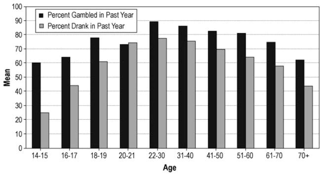
Gambling and alcohol use in past year by age

Figure 2 shows the significant age by gender interaction for any gambling in the past year. Males have high rates of gambling at a younger age than females. In the 20s and after, the rates are similar. Figure 3 shows the age by SES interaction. The age profile of gambling has a pronounced inverted U shape for the lower SES respondents; it is flatter for higher SES respondents.

Fig 2.

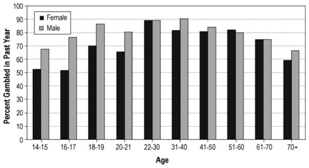
Gambling in past year: age by gender

Fig 3.

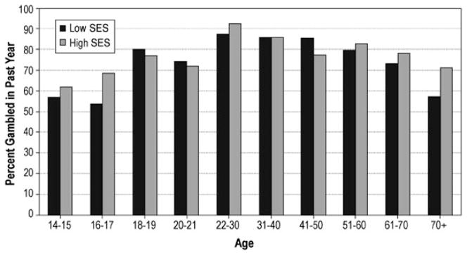
Gambling in past year: age by SES

Table 3 shows a logistic regression predicting frequent gambling (52+ times in the past year). Frequent gambling is highest in the age range 31–60 (see also Table 1). Figure 4 shows a comparison of the age profile of frequent gambling to the age profile of drinking .45 oz. of alcohol (about 1 drink) a day or more, an amount selected because it has the same proportion in the population as frequent gambling. The prevalence of drinking one drink a day or more peaks much younger (20–21 years) than frequent gambling, 51–60 years (Fig. 4). The odds of frequent gambling are higher for blacks and Native Americans than for whites, and lower SES respondents have higher odds of being a frequent gambler than higher SES respondents (Table 3; see also Table 1).

Fig 4.

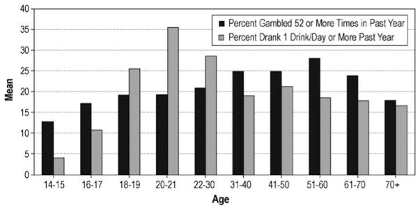
Alcohol use and gambling by age

Figure 5 shows the significant age by gender interaction for frequent gambling. For males, frequent gambling is near its highest prevalence by 18–19. For females, frequent gambling is not near its highest prevalence until the 30s.

Fig 5.

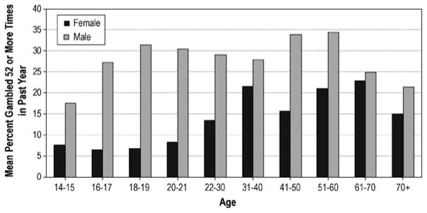
Frequent gambling: age by gender

Table 4 shows a logistic regression predicting problem gambling. The prevalence of problem gambling peaks at age 31–40, although the age range from youth to late middle age is not significantly different. Figure 6 shows a striking difference between the age profile of current problem gambling and the age profile of current alcohol dependence. At age 18–19 alcohol dependence peaks and has a prevalence over twice that of problem gambling. However, the age profile of alcohol dependence falls off quickly; and after age 21, problem gambling is more prevalent than alcohol dependence. For problem gambling, none of the age interactions were significant.

Fig 6.

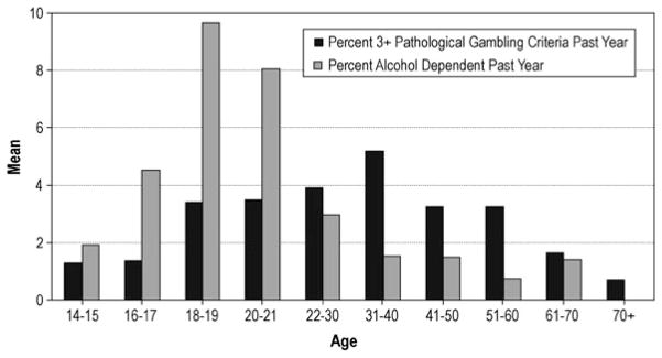
Alcohol dependence and problem gambling by age

Discussion

By combining two comparable national surveys of gambling among youths 14–21 and adults 18 and older, we were able to examine patterns of gambling and alcohol involvement across the lifespan. No comparable analysis has been done previously, and therefore none is available for a direct comparison. Our results do not support the notion that gambling involvement is highest in the teens (Shaffer et al. 1997). The percentage of respondents who gambled in the past year peaks in the age range 22–30, frequent gambling peaks in the 30s–50s, and problem gambling peaks at age 31–40. The percentage of respondents who drank in the past year also peaks at age 22–30, the same as the peak age for any gambling. However, the rate of drinking one drink per day or more peaks much younger than frequent gambling (20–21 vs. 31–60), and the rate of alcohol dependence peaks much younger than the rate of problem gambling (18–19 vs. 31–40). The extent of alcohol involvement falls off faster with age than does the extent of gambling involvement. The theory of Hirsch and Gottfredson, that deviant behaviors peak at an early age, seems to apply to alcohol more than it does to gambling.

In a recent analysis of data from our national youth gambling survey (Welte et al. 2009), we found that problem gambling had a much higher co-morbidity with conduct disorder if it started early in life. From this finding, we concluded that early-onset problem gambling had a closer link to general deviance than to late-onset problem gambling. This is consistent with the taxonomy advanced by Blaszczynski and Nower (2002), who proposed three etiology-based types of problem gambler: behaviourally conditioned, emotionally vulnerable, and antisocial impulsivist. The antisocial impulsivist is characterized by impulsivity, features of antisocial personality disorder, high rates of substance abuse, high rates of attention deficit hyperactivity disorder, and early onset of gambling involvement. Cloninger et al. (1996) made a similar observation about alcohol: they classified early-onset, highly anti-social and genetically influenced alcoholics as Type II, while those whose alcoholism emerged later in life and were not anti-social were classified as Type I. We speculate that a high proportion of problem gamblers are behaviourally conditioned (in Blaszczynski & Nower’s terminology) and analogous to Cloninger’s Type I alcoholic, and that the later-life development of those problem gamblers is responsible for fact that problem gambling peaks later in life than most problem behaviors.

Mok and Hraba (1991) suggested that the age-related decline in gambling involvement was due to the increasing social approval of gambling. It is certainly possible that the wave of legalization of gambling in recent decades, and the increase in the social approval of gambling, are responsible for the decline of gambling involvement with age. However, the age-related decline of gambling involvement is much slower than the age-related decline in alcohol involvement, and there has not been an increased availability of alcohol. It is therefore reasonable to speculate that the age-related decline in gambling is a developmental effect, and a part of the general decline in problem behaviors which occurs with age. Longitudinal data would be necessary to obtain convincing evidence.

Another interesting observation is that problem gambling has often been described as rare. Even the National Council on Problem Gambling (www.ncpgambling.org) describes it as ‘‘rare but treatable.’’ However, Fig. 6 shows that after age 21 problem gambling is considerably more common than alcohol dependence, although alcohol dependence has received much more attention. For example, there is no NIH agency dedicated to funding gambling research which is comparable to the National Institute on Alcohol Abuse and Alcoholism.

Unsurprisingly, males have more gambling involvement than females. Males reach their highest rates of any gambling and frequent gambling in the late teens, while females take longer to reach their highest rates. Clearly, male gambling involvement escalates earlier in life. It is also notable that frequent and problem gambling become more common as socioeconomic status gets lower. As we have speculated in our earlier work (e.g., Welte et al. 2004), lower SES Americans may be pursuing gambling as a way to make money, leading to more difficulties than if their motivation were strictly recreational. Native Americans are the highest or near highest on our three measures of gambling involvement, although this effect was statistically significant only for frequent gambling, due to a relatively small number of Native Americans in our sample.

In summary, gambling involvement is prevalent by middle adolescence, it increases through the 20s, and declines slowly until older adulthood when it falls off to a low level. Given the persistence of frequent gambling and problem gambling through adulthood, increased prevention and intervention efforts are warranted.

References

- American Psychiatric Association. DSM-IV: Diagnostic and Statistical Manual of Mental Disorders. 4. Washington, DC: American Psychiatric Association; 1994. [Google Scholar]
- Barnes GM, Welte JW, Hoffman JH, Tidwell MCO. Gambling, alcohol and other substance use among youth in the U.S. Journal of Studies on Alcohol and Drugs. 2009;70:134–142. doi: 10.15288/jsad.2009.70.134. [DOI] [PMC free article] [PubMed] [Google Scholar]
- Blaszczynski A, Nower L. A pathways model of problem and pathological gambling. Addiction. 2002;97:487–499. doi: 10.1046/j.1360-0443.2002.00015.x. [DOI] [PubMed] [Google Scholar]
- Cloninger CR, Sigvardsson S, Bohman M. Type I and type II alcoholism: An update. Alcohol Health & Research World. 1996;20:18–23. [PMC free article] [PubMed] [Google Scholar]
- Currie CE, Elton RA, Todd J, Platt S. Indicators of socioeconomic status for adolescents: The WHO Health Behaviour in School-aged Children Survey. Health Education Research. 1997;12:385–397. doi: 10.1093/her/12.3.385. [DOI] [PubMed] [Google Scholar]
- Ensminger ME, Forrest CB, Riley AW, Kang M, Green BF, Starfield B, et al. The validity of measures of socioeconomic status of adolescents. Journal of Adolescent Research. 2000;15:392–419. [Google Scholar]
- Gottfredson MR, Hirschi T. A general theory of crime. Stanford, CA: Stanford University Press; 1990. [Google Scholar]
- Grant BF. Prevalence and correlates of alcohol use and DSM-IV alcohol dependence in the United States: Results of the National Longitudinal Alcohol Epidemiologic Survey. Journal of Studies on Alcohol. 1997;58:464–473. doi: 10.15288/jsa.1997.58.464. [DOI] [PubMed] [Google Scholar]
- Hauser RM, Warren JR. Socioeconomic indexes for occupations: A review, update, and critique. Sociological Methodology. 1997;27:177–298. [Google Scholar]
- Hirschi T, Gottfredson MR, editors. The generality of deviance. New Brunswick, NJ: Transaction Publishers; 1994. [Google Scholar]
- Kallick M, Suits D, Dielman T, Hybels J. A survey of American gambling attitudes and behavior. Ann Arbor, MI: Institute for Social Research, The University of Michigan; 1979. [Google Scholar]
- Lavrakas PJ. Telephone survey methods: Sampling, selection, and supervision. Newbury Park, CA: Sage; 1993. [Google Scholar]
- Mok WP, Hraba J. Age and gambling behavior: A declining and shifting pattern of participation. Journal of Gambling Studies. 1991;7:313–335. doi: 10.1007/BF01023749. [DOI] [PubMed] [Google Scholar]
- National Opinion Research Center. Gambling impact and behavior study. Chicago, IL: NORC; 1999. [Google Scholar]
- Robins L, Marcus L, Reich W, Cunningham R, Gallagher T. NIMH Diagnostic Interview Schedule–Version IV (DIS-IV) St. Louis: Department of Psychiatry, Washington University School of Medicine; 1996. [Google Scholar]
- Shaffer HJ, Hall MN, Bilt JV. Estimating the prevalence of disordered gambling behavior in the United States and Canada: A meta-analysis. Boston, MA: Harvard Medical School; 1997. [DOI] [PMC free article] [PubMed] [Google Scholar]
- Stricker LJ. Measuring social status with occupational information: A simple method. Journal of Applied Social Psychology. 1988;18:423–437. [Google Scholar]
- Wardle J, Robb K, Johnson F. Assessing socioeconomic status in adolescents: The validity of a home affluence scale. Journal of Epidemiology and Community Health. 2002;56:595–599. doi: 10.1136/jech.56.8.595. [DOI] [PMC free article] [PubMed] [Google Scholar]
- Welte JW, Barnes GM, Tidwell MCO, Hoffman JH. The prevalence of problem gambling among U.S. adolescents and young adults: Results from a national survey. Journal of Gambling Studies. 2008;24:119–133. doi: 10.1007/s10899-007-9086-0. [DOI] [PMC free article] [PubMed] [Google Scholar]
- Welte JW, Barnes GM, Tidwell MO, Hoffman JH. The association between problem gambling and conduct disorder in a national survey of adolescents and young adults in the United States. Journal of Adolescent Health. 2009;45:396–401. doi: 10.1016/j.jadohealth.2009.02.002. [DOI] [PMC free article] [PubMed] [Google Scholar]
- Welte JW, Barnes GM, Wieczorek WF, Tidwell MCO, Parker J. Alcohol and gambling pathology among U.S. adults: Prevalence, demographic patterns and co-morbidity. Journal of Studies on Alcohol. 2001;62:706–712. doi: 10.15288/jsa.2001.62.706. [DOI] [PubMed] [Google Scholar]
- Welte JW, Wieczorek WF, Barnes GM, Tidwell MCO, Hoffman JH. The relationship of ecological and geographic factors to gambling behavior and pathology. Journal of Gambling Studies. 2004;20:405–423. doi: 10.1007/s10899-004-4582-y. [DOI] [PubMed] [Google Scholar]
- Winters KC, Henley GA. Adolescent Diagnostic Interview schedule and manual. Los Angeles, CA: Western Psychological Services; 1993. [Google Scholar]