A generalised enzyme kinetic model for predicting the behaviour of complex biochemical systems

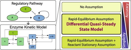
Graphical abstract

Highlights

• •We propose the dQSSA model as a novel way of modelling complex biological networks.
• •No low enzyme concentration assumption, covering more biological settings.
• •Reduces the number of parameters, which simplifies optimisation.
• •dQSSA was validated both in silico and in vitro.
• •Both biochemical and signalling pathways can be modelled accurately and simply.

Abstract

Quasi steady-state enzyme kinetic models are increasingly used in systems modelling. The Michaelis Menten model is popular due to its reduced parameter dimensionality, but its low-enzyme and irreversibility assumption may not always be valid in the in vivo context. Whilst the total quasi-steady state assumption (tQSSA) model eliminates the reactant stationary assumptions, its mathematical complexity is increased. Here, we propose the differential quasi-steady state approximation (dQSSA) kinetic model, which expresses the differential equations as a linear algebraic equation. It eliminates the reactant stationary assumptions of the Michaelis Menten model without increasing model dimensionality. The dQSSA was found to be easily adaptable for reversible enzyme kinetic systems with complex topologies and to predict behaviour consistent with mass action kinetics in silico. Additionally, the dQSSA was able to predict coenzyme inhibition in the reversible lactate dehydrogenase enzyme, which the Michaelis Menten model failed to do. Whilst the dQSSA does not account for the physical and thermodynamic interactions of all intermediate enzyme-substrate complex states, it is proposed to be suitable for modelling complex enzyme mediated biochemical systems. This is due to its simpler application, reduced parameter dimensionality and improved accuracy.

List of abbreviations

Model names

ODE

ordinary differential equation

tQSSA

total quasi-steady state assumption

dQSSA

differential quasi-steady state assumption

SBML

Systems Biology Markup Language

Chemical species

ATP

adenosine triphosphate

NAD⁺

nicotinamide adenine dinucleotide

NADH

reduced nicotinamide adenine dinucleotide

LDH

lactate dehydrogenase

Modelling states and parameters

S_F

free substrate

E_F

free enzyme

S_T

total substrate (sum of bound and free)

E_T

total enzyme (sum of bound and free)

ES

enzyme-substrate complex

EP

enzyme-product complex

P_F

free product

P_T

free product (sum of bound and free)

k

rate parameter

K^m

Michaelis constant

1. Introduction

Systems modelling of intracellular biochemical processes can provide quantitative insight into a cell’s response to stimuli and perturbations [1]. If the model is mechanistic, it has the power to both infer molecular mechanisms and predict biological responses [2]. This requires the simulation of biochemical reaction kinetics typically described using ordinary differential equations (ODEs). Modelling enzymatic cascade networks, however, requires the simulation of multiple reactions. This inevitably increases the complexity of the ODE model, which increases the number of free kinetic parameters. It then becomes more difficult to constrain all parameters simultaneously using a limited amount of available experimental data [3]. This can result in the derivation of multiple well fitting models with limited predictive power because of their non-uniqueness. Thus, an optimum parameter dimensionality should be selected to reduce non-uniqueness without reducing the topological complexity required to capture key kinetic features in the system [4].

Of the biochemical processes that need to be modelled, many are enzyme reactions [5]. Enzymatic cascades are based on enzyme kinetics within which additional interactions such as inhibition and allosteric effects can be included using mass action kinetics [6]. Basic enzyme kinetics is modelled using the following series of reactions:

$$S+E\underset{k_f^d}{\overset{k_f^a}{\rightleftharpoons }}\mathit{ES}\underset{k_f^c}{\overset{k_r^c}{\rightleftharpoons }}\mathit{EP}\underset{k_r^a}{\overset{k_r^d}{\rightleftharpoons }}P+E$$ (1)

where S, E, ES, EP and P denote the substrate, enzyme, enzyme-substrate complex, enzyme-product complex and product, respectively. The full mass action description of this reaction requires six kinetic parameters: k^a_f, k^d_f and k^c_f are the forward association, dissociation and catalytic rate parameters, respectively, and k^a_r, k^d_r and k^c_r are the corresponding reaction rate parameters in the reverse direction.

Many models of biochemical systems use the simplified irreversible form of the reaction (Fig. 1d), which only requires three kinetic parameters [5,7–15]. Whilst this is an approximation of real enzyme action, in vitro spectroscopic studies of single molecule enzyme kinetics have shown that this approximation is sufficient in experiments where there is no product inhibition [16,17]. Further simplifications have led to other enzyme kinetic models such as the Michaelis–Menten model and the Tzafriri total quasi-steady state assumption (tQSSA) model [7,9,18–21]. Whilst the Michaelis–Menten model is more widely used, it is strictly accurate at low enzyme concentrations. Since this may not be true under in vivo conditions, unrealistic conclusions may be drawn from models using the Michaelis–Menten equation [18,22–24]. The tQSSA is not subject to the same limitation, but it has a more complex mathematical form that requires reanalysis for each distinct network to which it is applied [24]. Currently, systems modellers must choose between complex enzyme models with high parameter dimensionality, or simpler models at the cost of accuracy.

Fig. 1.

Various models of enzyme kinetics in a cyclic reaction system. (a) Shows the simple reaction cycle which interconverts a substrate and product involving an enzyme reaction and a backward decay reaction. (b) Shows the mechanism of the reversible enzyme kinetic model, (c) shows the coupled irreversible enzyme kinetic model, (d) shows the irreversible enzyme kinetic model, which includes the Michaelis Menten model and tQSSA model.

A further compounding factor is that in vitro investigations of enzyme action are generally performed in closed thermodynamic systems which achieve thermodynamic equilibrium, as reflected in the model described by Eq. (1). Cellular systems, however, are not thermodynamically closed, and so achieve only homeostatic equilibrium. This is achieved by constant energy inflow through coenzymes such as ATP which allows the network to form cyclic reactions made of counteracting enzymatic reaction pairs which maintain and regulate this equilibrium. Examples of cyclic reactions are the cyclic interconversion of nicotinamide adenine dinucleotide (NAD⁺) and nicotinamide adenine dinucleotide phosphate (NADP⁺), mediated by NAD kinase and NADP⁺ phosphatase in metabolism, and the cyclic interconversion of phosphatidylinositol (4,5)-bisphosphate to (3,4,5)-triphosphate, mediated by PI3K kinase and PTEN phosphatase in insulin and cancer signalling [25–27]. Thus, models of cellular systems need to account for the continual energy consumption in these cyclic reactions. Conventionally, the global coenzyme concentration is not the focus of study, hence systems models implicitly account for the effects of coenzyme concentration [CoE] by asserting that $k_c^{\prime }\approx k_c[\text{CoE}]$ and then directly varying the catalytic rate $k_c^{\prime }$ to vary energy input rate. This allows the thermodynamically closed enzyme kinetic model to be used in a thermodynamically open context [4].

To address these issues, we have developed a generalised enzyme kinetic model that retains its mathematical form for systems with multiple enzymes, whilst minimising the number of simplifying assumptions and parameters needed to characterise the system. This enables more accurate simulation of the biochemical mechanisms involved.

2. Theoretical background

As enzymes form the basis of many biochemical processes, models of enzyme kinetics are fundamental components of mathematical models of biochemical networks. The difficulty in implementing enzyme kinetic models lies in its variety in the literature. In this section, we demonstrate and compare the limits of various simplifications of enzyme kinetic model, beginning with the more complex mass action based reversible enzyme kinetic model in a reaction cycle. The reaction cycle will involve an enzymatic reaction that favours substrate to product formation, coupled with an irreversible decay reaction of the product back to substrate (Fig. 1).

Whilst the overall goal of this work is to achieve an optimally accurate dynamic model, in this section, we focus on the product concentration at homeostatic equilibrium, or complete steady state as the standard of comparison. This is because the homeostatic, product concentration is easier to compare analytically than the full temporal behaviour, but an incorrect homeostatic equilibrium state implies the kinetic behaviour of the model is incorrect.

The following notations are used throughout:

• (i)Species names enclosed in square brackets implies their concentration, e.g. [S_F] is the concentration of S_F.
• (ii)Overhead dots of state variables indicate the total time derivative. e.g. $[{\dot{S}}_F]=d[S_F]/\mathit{dt}$ .
• (iii)Subscript T of states variables indicate total (free and in complex) concentrations of the parent species e.g. $[S_T]=[S_F]+[\mathit{ES}]$.
• (iv)Subscript 0 of state variables indicates initial concentrations of the parent species e.g. $[S_F(t=0)]={[S_F]}_0$.
• (v)Subscript ∞ of state variables indicates steady state concentrations of the parent species e.g. $[S_F(t=\infty )]={[S_F]}_{\infty }$.
• (vi)Numerical subscript of rate parameters indicates the reaction number it belongs to; additional subscripts such as f or r indicate the rate parameter in the forward or reverse direction of the enzyme reaction, or other labels for other types of rate parameters. Superscript a, d, or c on a rate parameter indicates the association, dissociation and catalytic rates of the enzyme reaction and direction given by the subscript respectively e.g. $k_{1f}^c$ indicates the catalytic rate parameter for reaction 1 in the forward direction.
• (vii)Parameters in bold font denote tensors and their numerical subscripts indicate their indices.

2.1. Reversible enzyme kinetic model in a cyclic reaction system

For the reversible cyclic reaction shown in Fig. 1b, the mass action model can be expressed minimally as [6,28]:

$$[\stackrel{·}{\mathit{ES}}]=k_{1f}^a[S_F][E_F]+k_{1r}^c[\mathit{EP}]-(k_{1f}^d+k_{1f}^c)[\mathit{ES}]$$ (2)

$$[\stackrel{·}{\mathit{EP}}]=k_{1r}^a[P_F][E_F]+k_{1f}^c[\mathit{ES}]-(k_{1r}^d+k_{1r}^c)[\mathit{EP}]$$ (3)

$$[\stackrel{·}{P_F}]=-k_{1r}^a[P_F][E_F]+k_{1r}^d[\mathit{PE}]-k_2[P_F]$$ (4)

$${[S_T]}_0=[S_F]+[P_F]+[\mathit{ES}]+[\mathit{EP}]$$ (5)

$${[E_T]}_0=[E_F]+[\mathit{ES}]+[\mathit{EP}]$$ (6)

Setting all derivatives to zero, solving Eqs. (2) and (3) simultaneously, and then substituting the result into Eq. (4), leads to the following expression for the free product concentration at complete steady state:

$${[P_F]}_{\infty }=\frac{1}{k_2}\frac{k_f^c{\beta }_r\frac{{[E_F]}_{\infty }{[S_F]}_{\infty }}{K_{\mathit{mS}}}(1-{\alpha }_f{\alpha }_r)-k_r^c{\beta }_f\frac{{[E_F]}_{\infty }{[P_F]}_{\infty }}{K_{\mathit{mP}}}(1-{\alpha }_f{\alpha }_r)}{({\beta }_r+{\beta }_f{\alpha }_r)({\beta }_f+{\beta }_r{\alpha }_f)}$$ (7)

where

$${\alpha }_i=\left(\frac{k_i^c}{k_i^c+k_i^d}\right|{\beta }_i=\frac{k_i^d}{k_i^c+k_i^d}$$ (8)

and

$$K_i^m=\frac{k_i^c+k_i^d}{k_i^a}$$ (9)

is the conventional Michaelis constant and i indicates whether the constant is associated with the forward or reverse reaction. Note that this expression for the equilibrium product concentration is different from the result from conventional derivations as we have retained the use of the free enzyme concentration as our variable and have applied an additional unimolecular decay reaction from product to substrate, which modifies the resulting expression (see Doc S1 for results obtained using conventional methods). We also note that this model creates eight coefficients; therefore all six kinetic parameters are needed to fully define the coefficients and the model.

2.2. Irreversible enzyme kinetic models in cyclic reactions

The coupled irreversible cyclic reaction shown in Fig. 1c is similar to the full reversible system with a subtle difference. The catalysis step of both the forward and reverse reactions immediately dissociate into their respective end species and free enzyme. The purpose of making this subtle change is to make the reversible reaction appear like two coupled irreversible enzyme reactions, which can be expressed minimally as:

$$\stackrel{·}{[\mathit{ES}]}=k_{1f}^a[E_F][S_F]-(k_{1f}^c+k_{1f}^d)[\mathit{ES}]$$ (10)

$$\stackrel{·}{[\mathit{EP}]}=k_{1r}^a[E_F][P_F]-(k_{1r}^c+k_{1r}^d)[\mathit{EP}]$$ (11)

$$[{\dot{P}}_F]=-k_{1r}^a[P_F][E_F]+k_{1r}^d[\mathit{EP}]+k_{1f}^c[\mathit{ES}]-k_2[P_F]$$ (12)

$${[S_T]}_0=[S_F]+[P_F]+[\mathit{ES}]+[\mathit{EP}]$$ (13)

$${[E_T]}_0=[E_F]+[\mathit{ES}]+[\mathit{EP}]$$ (14)

Again, setting all derivatives to zero and substituting Eq. (10) and (11) into Eq. (12), leads to the following expression for the free product concentration at complete steady state of the coupled irreversible system.

$${[P_F]}_{\infty }=\frac{1}{k_2}\left(\frac{k_{1f}^c{[S_F]}_{\infty }{[E_F]}_{\infty }}{K_S^m}-\frac{k_{1r}^c{[P_F]}_{\infty }{[E_F]}_{\infty }}{K_P^m}\right)$$ (15)

where $K_S^m$ and $K_P^m$ are the Michaelis constants for the forward and reverse reactions respectively. This is similar to the analogous expression for the fully reversible system (Eq. (7)) under the conditions $k_{1f}^d\gg k_{1f}^c$ and $k_{1r}^d\gg k_{1r}^c$ which causes ${\alpha }_f\text{,}{\alpha }_r\approx 0$, and ${\beta }_f\text{,}{\beta }_r\approx 1$, which is required for Eq. (7) to become identical to Eq. (15). This implies that under the “rapid equilibrium” condition (where free enzymes and substrates rapidly equilibrate with their complexed forms) the reversible enzyme kinetic system can be modelled as two opposing irreversible enzyme kinetic systems losing mechanistic detail. This assumption is identical to the original quasi-steady state assumption made by Michaelis and Menten [29].

For the reaction to be completely irreversible (Fig. 1d), we simply set $k_r^c=0$. This leads to the following result for the product concentration at complete steady state:

$${[P_F]}_{\infty }=\frac{k_{1f}^c}{k_2}\frac{{[S_F]}_{\infty }{[E_F]}_{\infty }}{K_S^m}$$ (16)

This model is now less realistic as enzymes do not behave irreversibly under physiological conditions. A significant consequence is that this model no longer includes product inhibition since no enzyme-product complex exists. For the purpose of comparison, however, we will require this result for the following sections.

2.3. The Michaelis–Menten model in cyclic reactions

Whilst the Michaelis–Menten (and Briggs–Haldane) model is a subset of the irreversible enzyme kinetic model, it is worthy of a standalone analysis as it is widely used in models of biochemical systems. Since the topology of reaction networks can itself be complicated, this model is often used to simplify the mathematics of the network model [5,8–12]. However, the mechanistic accuracy of the Michaelis–Menten model can break down under physiological conditions, such as for protein phosphorylation networks.

The Michaelis–Menten model adopts the quasi-steady state assumption, where the enzyme-substrate complex [ES] is set to be constant over small time scales ($[\dot{\mathit{ES}}]=0$ in Eq. (10)). This leads to the following expression for the enzyme-substrate complex:

$$[\mathit{ES}]=\frac{[S_F][E_F]}{K_S^m}$$ (17)

The state variable used is total enzyme concentration rather than free enzyme using the following substitution [7]:

$${[E_T]}_0=[E_F]+[\mathit{ES}]$$ (18)

Combining Eqs. (16)–(18) leads to the following expression for the enzyme reaction rate v is then:

$$v=k_{1f}^c\frac{{[E_T]}_0[S_F]}{K^m+[S_F]}$$ (19)

And the resulting kinetic equations for our cyclic reaction system using this enzyme kinetic model can be expressed as [9]:

$$[{\dot{S}}_F]=-\frac{k_{1f}^c{[E_T]}_0[S_F]}{K_S^m+[S_F]}+k_2[P_F]$$ (20)

$$[{\dot{P}}_F]=\frac{k_{1f}^c{[E_T]}_0[S_F]}{K_S^m+[S_F]}-k_2[P_F]$$ (21)

$${[S_T]}_0=[S_F]+[\mathit{ES}]+[P_F]$$ (22)

The product concentration at complete steady state is thus:

$${[P_F]}_{\infty }=\frac{k_{1f}^c}{k_2}\frac{{[S_F]}_{\infty }{[E_T]}_0}{K_S^m+{[S_F]}_{\infty }}$$ (23)

This is similar to Eq. (16) expressed in terms of ${[E_T]}_0$ by substituting in Eqs. (17) and (18). So in principle the Michaelis–Menten model is consistent with the mass action based irreversible enzyme kinetics model. In practice, however, this is not the case because it is commonly assumed that:

$$[S_F]\approx [S_T]$$ (24)

This implies that the ES complex must have a negligible concentration:

$$[\mathit{ES}]\approx 0$$ (25)

This is known as the reactant stationary assumption and is the origin of the low enzyme assumption implicit in the Michaelis–Menten model [9,23,30–32]. The condition required for this assumption to hold true is given by [18,32]:

$${[E_T]}_0<K_S^m+{[S_T]}_0$$ (26)

This does not strictly require that ${[E_T]}_0<<{[S_T]}_0$ but in the situation where ${[E_T]}_0⩾{[S_T]}_0$, a low enzyme-substrate affinity associated with a large $K_S^m$ is instead required for condition Eq. (25) to hold [32,33]. The tQSSA proposed by Tzafriri avoids this limitation by implicitly accounting for the enzyme-complex concentration by re-expressing the series of equations in terms of the total substrate concentration $[S_T]$ [18].

Despite this, there is a second way both models can further lose accuracy. In a system where an enzyme has multiple targets (e.g. Akt), the substitution in Eq. (18) is no longer valid [34]. This causes both the Michaelis–Menten and tQSSA models to break down as they both rely on this conservation law. Hence, the rate equations for these quasi-steady state models need to be rederived for each distinct biochemical network. As shown in other studies involving analysis using the tQSSA, this can become impractical as the networks become complex enough that the ensuing simultaneous equations become analytically intractable [24].

3. Results

We have established that reversible enzyme kinetics can be approximated as two opposing irreversible enzyme reactions under rapid equilibrium conditions. We also showed that the Michaelis–Menten quasi-steady state assumption fails to accurately reflect the mass action irreversible enzyme reaction since the enzyme-substrate concentration is not properly accounted for as a result of the reactant stationary assumption. If the quasi-steady state complex concentration can be dynamically calculated using a generalised method, the reactant stationary assumption would no longer be needed. Thus the rapid equilibrium assumption would be the only assumption made which will increase model accuracy (see Doc S1 for justification of why this cannot be achieved with the fully reversible model). Our approach proposes to achieve this by linearising the quasi-steady state model such that the complex state (made implicit by the quasi-steady state assumption) can be explicitly calculated at each integration step. This approach is henceforth referred to as the differential quasi-steady state assumption (dQSSA).

In this section, we first describe the mathematics behind the dQSSA model. Next we validate the model in silico and demonstrate its application by applying it to a complex hypothetical network and comparing its predicted time course to that achieved by the mass action and Michaelis–Menten models. Finally, we experimentally validate the dQSSA by applying it to the interconversion of pyruvate and lactate by lactate dehydrogenase (LDH) in the presence of different concentrations of coenzyme and enzyme. This will demonstrate the performance of this model and its ability to mechanistically predict the behaviour of a realistic biochemical system under physiological conditions.

3.1. Development of the dQSSA

The primary challenges the dQSSA must meet are threefold:

• (1)Calculation of state variables in a complex enzyme kinetic system without solving any simultaneous equations;
• (2)Retain the accuracy and parameter reduction on par with the tQSSA irreversible enzyme kinetic model;
• (3)Simplify the conversion between network topology into a dynamic equation.

Starting with the quasi-steady state assumption of Eq. (17), we note that the act of taking the quasi-steady state forces the ES complex concentration to only be a function of the enzyme and substrate concentrations, i.e. $\partial C/\partial t=0$ (see Doc S2). Note that, in general, the enzyme and substrate concentrations (both free and total) are themselves functions of time. Thus, the total time derivative of the complex concentration (i.e. of Eq. (10)) is not always zero. In fact, it is:

$$[\stackrel{·}{\mathit{ES}}]=\frac{[S_F]}{K_S^m}[\stackrel{·}{E_F}]+\frac{[E_F]}{K_S^m}[\stackrel{·}{S_F}]$$ (27)

Now differentiating the conservation laws for the enzyme and substrate states by time produces the following differential equations for the free enzyme and substrates:

$$[\stackrel{·}{E_f}]=-[\stackrel{·}{\mathit{ES}}]$$ (28)

$$[\stackrel{·}{S_F}]=-[\stackrel{·}{P_F}]-[\stackrel{·}{\mathit{ES}}]$$ (29)

Substituting the differential equation for the ES complex (Eq. (27)) into Eqs. (28) and (29) leads to the quasi-steady state assumption for the four state variables of the system in differential form.

$$[{\dot{P}}_F]=k^c[\mathit{ES}]$$ (30)

$$[{\dot{S}}_F]=-k^c[\mathit{ES}]-\frac{[S_F]}{K_S^m}[{\dot{E}}_F]-\frac{[E_F]}{K_S^m}[{\dot{S}}_F]$$ (31)

$$[{\dot{E}}_F]=-\frac{[S_F]}{K_S^m}[{\dot{E}}_F]-\frac{[E_F]}{K_S^m}[{\dot{S}}_F]$$ (32)

$$[\stackrel{·}{\mathit{ES}}]=\frac{[S_F]}{K_S^m}[\stackrel{·}{E_F}]+\frac{[E_F]}{K_S^m}[\stackrel{·}{S_F}]$$ (33)

Unfortunately, this series of equations are implicit because the derivatives are now mixed. Further manipulation into an explicit form requires re-expressing the linear system of differential equations as a vector $x$ of state variables. Using the indices:

• (1)Substrate
• (2)Enzyme
• (3)Product
• (4)ES complex

and isolating all derivatives to the left hand side leads to:

$$\left(1+\frac{x_2}{K_S^m}\right){\dot{x}}_1+\frac{x_1}{K_S^m}{\dot{x}}_2=-k^c{x}_4$$ (34)

$$\frac{x_2}{K_S^m}{\dot{x}}_1+\frac{x_2}{K_S^m}\left(1+\frac{x_1}{K_S^m}\right){\dot{x}}_2=0$$ (35)

$${\dot{x}}_3=k^c{x}_4$$ (36)

$$-\frac{x_2}{K_S^m}{\dot{x}}_1-\frac{x_1}{K_S^m}{\dot{x}}_2+{\dot{x}}_4=0$$ (37)

which can then be linearised as:

$$({\delta }_{\mathit{ij}}+{\mathbf{G}}_{\mathit{ijk}}{x}_k){\dot{x}}_j={\mathbf{W}}_{\mathit{ij}}{x}_j$$ (38)

where ${\delta }_{\mathit{ij}}$ is the Kronecker delta, and

$${\mathbf{G}}_{\mathit{ijk}}=\left\{\begin{array}{c}\hfill 1/K_S^m\hfill \\ \hfill -1/K_S^m\hfill \\ \hfill 0\hfill \end{array}\right)\begin{array}{c}\hfill \text{if}[i\text{,}j\text{,}k]=[1\text{,}1\text{,}2]\text{,}[1\text{,}2\text{,}1]\text{,}[2\text{,}1\text{,}2]\text{,}[2\text{,}2\text{,}1]\hfill \\ \hfill \text{if}[i\text{,}j\text{,}k]=[4\text{,}1\text{,}2]\text{,}[4\text{,}2\text{,}1]\hfill \\ \hfill \text{Else}\hfill \end{array}$$ (39)

$${\mathbf{W}}_{\mathit{ij}}=\left\{\begin{array}{c}\hfill -k^c\hfill \\ \hfill k^c\hfill \\ \hfill 0\hfill \end{array}\right)\begin{array}{c}\hfill \text{if}[i\text{,}j]=[1\text{,}4]\hfill \\ \hfill \text{if}[i\text{,}j]=[3\text{,}4]\hfill \\ \hfill \text{Else}\hfill \end{array}$$ (40)

The derivative terms can then be isolated from the non-derivative terms, leading to:

$${\dot{x}}_k={({\delta }_{\mathit{ij}}+{\mathbf{G}}_{\mathit{ijk}}{x}_k)}^{-1}{\mathbf{W}}_{\mathit{ij}}{x}_j$$ (41)

Multiple enzymatic reactions can be modelled simultaneously by adding the differential equation for each enzyme’s ES complex into the differential equation for their corresponding enzyme and substrate (i.e. Eqs. (28) and (29) respectively). For example, an enzyme that targets two substrates will be governed by the following dynamic equation:

$$[{\dot{E}}_F]=-\frac{[E_F]}{K_1^m}[{\dot{S}}_{F1}]-\frac{[E_F]}{K_2^m}[{\dot{S}}_{F2}]-\frac{[S_{F1}]}{K_1^m}[{\dot{E}}_F]-\frac{[S_{F2}]}{K_2^m}[{\dot{E}}_F]$$ (42)

This additional process can be implemented directly through the tensors. For n number of reactions within a network, the global dynamic equation is simply constructed by performing element by element summation of corresponding tensors from each individual enzymatic reaction r:

$${\mathbf{G}}_{\mathit{ijk}}^{(\text{Global})}={\displaystyle \sum _r^n}{\mathbf{G}}_{\mathit{ijk}}^{(r)}$$ (43)

$${\mathbf{W}}_{\mathit{ij}}^{(\text{Global})}={\displaystyle \sum _r^n}{\mathbf{W}}_{\mathit{ij}}^{(r)}$$ (44)

The dynamic equation can also be generalised to include other reactions. Fundamental unimolecular and bimolecular reactions, if included, would appear as an additional sum on the right hand side of Eq. (41). An external input can be implemented as an arbitrary function of the time and state variables, which appears on the right hand side of the equation. Thus, the fully generalised equation, which includes other reactions, is:

$${\dot{x}}_k={({\delta }_{\mathit{ij}}+{\mathbf{G}}_{\mathit{ijk}}{x}_k)}^{-1}[{\mathbf{V}}_{\mathit{ijk}}{x}_i{x}_j+{\mathbf{W}}_{\mathit{ij}}x+{\sigma }_i(t)+f_i(t\text{,}\overrightarrow{x})]$$ (45)

where ${\mathbf{V}}_{\mathit{ijk}}$ is a three dimensional tensor containing bimolecular rate constants, ${\mathbf{W}}_{\mathit{ij}}$ is a two dimensional tensor containing unimolecular rate constants, ${\sigma }_i$ is a one dimensional tensor containing synthesis type rate parameters and $f_i(t\text{,}\overrightarrow{x})$ is a vector of arbitrary functions of external inputs or other kinetic models. We refer to Eq. (45) as the dQSSA. By expressing the kinetic equation in this way, the model topology is now captured by the location and value of non-zero tensor elements.

What remains is a method for calculating the initial conditions for the quasi-steady state system. As the equation uses free and bound forms as state variables, it is initially unknown how much of the system’s reactants are bound within the complex for example. What is known instead is the total concentration of each species. Thus distribution of the total concentration into free and bound parts can be determined by simulating the addition of the total concentrations into an empty system using the dynamic equation (Eq. (45)). If the addition is made much faster than the reactions in the system, then the complex formation can be separated from the system’s evolution. As an in silico system, it is possible to simulate an infinitely fast addition. This is done by setting all terms within the square brackets of Eq. (45) to zero, which stops all non complex formation reactions from taking place. The system’s transient initial concentrations can then be “injected” into the system through the $f_i(t\text{,}\overrightarrow{x})$ parameter using an injection profile $q_{\text{ssa}}(t)$ (i.e. $q_{\text{ssa}}(t)=f_i(t\text{,}\overrightarrow{x})$). This is the only term within the square bracket that will be non-zero. The idea is the initial total concentrations are injected into the system which is allowed to equilibrate into its quasi-steady state without the transient non-quasi-static reactions explicitly running.

The only requirement for the input profile $q_{\text{ssa}}(t)$, is that ${\int }_0^{t_{\text{end}}}{q}_{\text{ssa}}(t)\mathit{dt}=x_0$ where $t_{\text{end}}$ is the end time of the additional simulation. This requirement states that the integrated rate of addition equals the total initial concentration. In practice, a Gaussian profile achieves the most accurate result due to its initially slow increase which minimises numerical error. The resulting steady state from this simulation defines the quasi-steady state initial concentrations of the kinetic simulation.

3.2. In silico validation

Whilst one of the goals of the dQSSA is to maximise the mechanistic accuracy of individual enzymatic reactions, this is secondary to the primary goal of achieving reliable predictions of the behaviour of arbitrarily large enzyme networks. This was verified by benchmarking the dQSSA against the predictions made by the mass action implementation of the same network. As the mass action model is mathematically verbose, this presents a practical limit on the size of the network that can be conveniently tested. Thus, a hypothetical small but complex network was designed such that it can be practically implemented whilst achieving the two verification goals.

The network was designed with an activator I which flips the network between two regimes (Fig. 2). The first regime (the I-off network), is designed to satisfy the simpler secondary goal of mechanistic accuracy. The only active reactions are unimolecular, bimolecular and a reversible enzyme reaction (the reverse reaction for reaction 10 is technically active in the I-off network, but as it is unfavoured, its effects are mostly negligible). This allows us to isolate the performance of the dQSSA within a controlled enzymatic system. A separate arm also tests the dQSSA’s ability to model fundamental reactions. The second regime (the I-on network), opens the network to topological complexity which allows us to assess the ability of the dQSSA to handle networks with complex coupling between reactions. The following coupling mechanisms were tested:

• •An enzyme with two substrate targets.
• •A substrate that is targeted by two enzymes.
• •A substrate that is itself an enzyme.

Fig. 2.

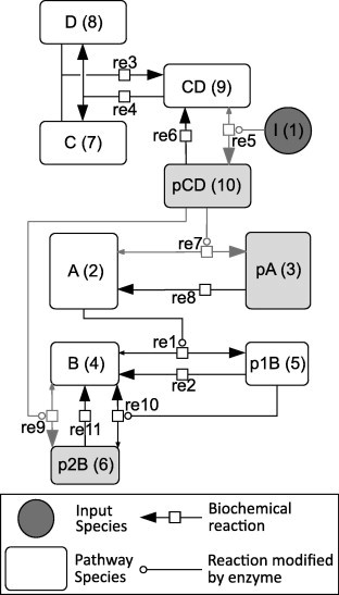
The hypothetical network constructed for in silico model validation. Network is illustrated in accordance for the Systems Biology Graphical Notation (SBGN) [45]. (A, B) and (C, D) Belong to two different pathways which cross-talk when I (circular species) is added. This activates shaded reactions and enables formation of shaded species. The numbers in parentheses next to the species refer to their indices in the model equations in the computational program (Doc S5).

The kinetic parameters for the reactions in this hypothetical model were mostly randomly generated, with the exception of the following:

• •The catalytic rate of the enzymatic reaction designated as the “forward reaction” is always larger than the direction designated as the “reverse reaction”.
• •The rapid equilibrium condition is enforced by setting the two dissociation rate constants of an enzymatic reaction to be one hundred times larger than the two catalytic rates of the reversible enzyme reaction.
• •So as to not unnecessarily bias the Michaelis constants of the reaction, the two randomly generated enzyme-substrate association rate constants are also made one hundred times larger than their randomised values.

This was done in order to benchmark the models in a parameter independent way.

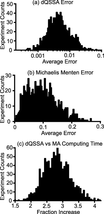
In the one thousand randomly generated parameter sets, the dQSSA model closely matched the time course of the mass action models, both in the I-off network and I-on network. At equilibrium, the average percentage difference between the two models was 0.5% over 1000 simulations (Fig. 4a, representative time courses shown in Doc S3) This I-off network verified that the dQSSA can replicate the mass action based reversible enzyme model whilst the I-on network showed that the dQSSA can accurately model the system behaviour with complex couplings in the network. We also investigated the performance of the Michaelis–Menten model in this scenario. We found that in many cases, the Michaelis–Menten model was inconsistent with the mass action and dQSSA model results, with an average difference of 9.7% over 1000 simulations (Fig. 4b, representative time courses shown in Doc S3).

Fig. 4.

Average error and computing times over multiple in silico runs. Histograms showing the (a) average fraction error between the dQSSA and mass action models, (b) average error between the Michaelis–Menten and mass action models, (c) spread of dQSSA compute time over mass action compute time, across 1000 computation runs. For (a) and (b), larger values are worse as they indicate a larger average difference between model predictions. For (c), smaller values are better as this indicates a better computational efficiency in simulating the system.

As seen in the theoretical analysis, this is most likely due to a violation of the low enzyme assumption of Eq. (26). Therefore, we further investigated whether this inconsistency requires the low enzyme assumption to be violated throughout the whole network, or whether a single instance is sufficient to cause inaccuracies in the whole network. To investigate this, we tested parameters such that the low enzyme assumption in all reactions except the forward direction of reaction 9. As such, the Michaelis–Menten model should be consistent with the other two models during the I-off phase but inconsistent in the I-on phase. The parameters used are given in Table 1. We found that all three models were consistent during the I-off phase (Fig. 3). However, in the I-on phase, the dQSSA and mass action model remained consistent with each other whilst the Michaelis–Menten model became inconsistent and varied between 7% and 45% consistency at equilibrium. The A and pA states had a difference of approximately 20% even though these are not directly related to the species involved with the high enzyme concentration reaction. Hence, this result demonstrates that violation of the low enzyme assumption even in just one reaction can lead to non-trivial discrepancies in the Michaelis–Menten model’s predictions.

Table 1.

Parameters of the in silico system. Parameters used for the in silico validation result shown in Fig. 3.

Fig. 3.

In the hypothetical network, the dQSSA is consistent with mass action kinetics whilst the Michaeli–Menten model is not. Time courses of the network simulation were predicted by the mass action model (crosses), Michaelis–Menten model (pluses) and dQSSA model (crosses). The total (i.e. free and in complex) concentration of each species are shown to enable a fair comparison between models (a–c). I is only added at t = 10 s (d).

Whilst the dQSSA was found to be significantly better than the Michaelis–Menten model at matching the mass action model’s predictions, the linearisation of the dynamic equation and the inclusion of a matrix inversion increases the model’s computational cost. For example, in our hypothetical network, we found that the dQSSA model (including solving for the initial conditions) required approximately 3 times longer to solve when compared to the mass action model (Fig. 4c). The accuracy of the dQSSA for estimating kinetic parameters was also tested by fitting the dQSSA model to the mass action generated time course with artificial noise with signal to noise ratio of 5 was added. It was found that fitted parameters are at most different by an average of 20% and the uncertainty of the fitted parameters covers the true parameter value (see Doc S3). This demonstrates that the dQSSA is useful in parameter estimation against experimental time course data.

3.3. Experimental validation

Thus far, the in silico validation demonstrated good agreement between the mass action model and the dQSSA whilst highlighting the deficiency in the Michaelis–Menten model. To determine its practical significance, we extended our comparison to an in vitro setting, modelling the action of LDH.

LDH is a well-characterised enzyme which reversibly converts pyruvate and reduced nicotinamide adenine dinucleotide (NADH) to lactate and NAD⁺. The reaction mechanism for LDH (Fig. 5) involves the ordered binding of the coenzymes (NADH or NAD⁺) to LDH followed by the subsequent binding of its corresponding substrate (pyruvate or lactate, respectively) [35]. The transfer of an electron between the coenzyme and the substrate then reversibly occurs in the ternary complex as part of the catalytic process. As LDH appears to be an enzyme that satisfies the “rapid equilibrium” assumption, this reversible catalysis can be viewed as two distinct reactions as described in Section 2.2 [36]. Thus, it is ideal for verifying whether the in silico difference found between the dQSSA model and the Michaelis–Menten model seen in Section 3.2 translates in vitro.

Fig. 5.

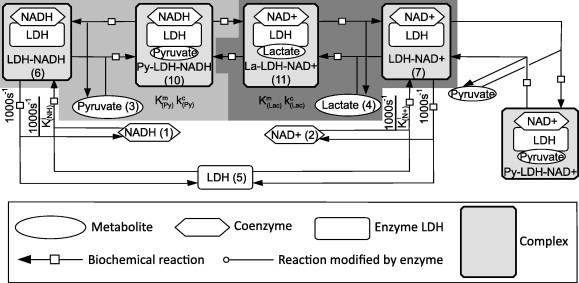
The model mechanism of LDH binding. Network is illustrated in accordance for the SBGN. The numbers denote the species ID in the mathematical model. The light grey and dark grey regions make up the enzymatic reactions that are abstracted by the dQSSA and Michaeli–Menten models. The kinetic parameters associated with them are shown in the shaded region. The remaining reactions adapted from [35].

As this is a real system, the first step involved characterising the kinetic constants in both directions. The reactions were run in the irreversible regime by adding equimolar concentrations of the reactant and coenzyme of the relevant reaction direction. The constants were then obtained by least squares fitting of the initial concentration and reaction velocity using a Lineweaver Burk plot (Fig. 6a and b). The time course of the reaction was run with a low time resolution to smooth out the kinetics of the transient phase, and the reaction velocity was calculated using the first 5 time points to smooth out other experimental noise that can skew this parameter The dissociation constants of the coenzymes were then determined by fitting the predicted time course with the experimental time course, which describes the kinetics of the system when all four reactants are present. Four representative fits are shown in Fig. 6c–f (see Doc S4 for the full set of data used). This approach was taken as the progression of the reaction caused all four reactants to become present. We reasoned that this causes the effect of coenzyme competition for the LDH to become present, which can be used to determine the dissociation constants. The resulting parameters are shown in Table 2 and were found to be in good agreement with that found in the literature [37,38].

Fig. 6.

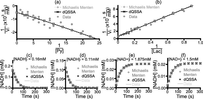
Derivation of the LDH kinetic parameters. The Lineweaver–Burk plot for the (a) pyruvate to lactate reaction and (b) lactate-to-pyruvate reaction, with the best fit line used to determine $K^m$ and $k^c$ (Table 2). (c)–(f) Representative time courses used for fitting the $K^i$ for coenzymes. The remaining time courses used are presented in Figs. S1–4.

Table 2.

Parameters and residuals of LDH system. Parameters used for the in vitro LDH system shown in Fig. 6 and the residuals for the best fit used to obtain them.

	Michaelis–Menten		dQSSA (value)
	Value	Residual	Value	Residual
NADH $K_{\left(\text{NH}\right)}^i$ (M)	9.23 × 10−9	4.2 × 104	9.83 × 10−9	3.0 × 104
NAD+$K_{\left({\text{NH}}^{+}\right)}^i$ (M)	3.79 × 10−7	N/A	3.79 × 10−7	N/A
$K_{\left(\text{Py}\right)}^m$ (mM)	1.25 × 10−4	9.5 × 105	1.27 × 10−4	9.5 × 105
$k_{\left(\text{Py}\right)}^c$ (s−1)	78.9		79.3
$K_{\left(\text{Lac}\right)}^m$ (mM)	1.30 × 10−2	2.0 × 106	1.35 × 10−2	2.0 × 106
$k_{\left(\text{Lac}\right)}^c$ (s−1)	62.8		63.3

At this point, it was necessary to verify the generated model. It is expected that when a reaction is initiated in a single direction, the presence of the opposing coenzyme will cause inhibition as some enzyme is bound with the wrong coenzyme. Given the quantitative nature of the dQSSA model, the degree of inhibition should be correctly predicted by the two models. As such, prediction of the change in initial reaction velocity of the pyruvate to lactate reaction, under varying concentration of NAD⁺ was used as the validating experiment. A good agreement was found between the dQSSA model’s prediction and the observed result (Fig. 7). On the other hand, the Michaelis–Menten model gave a different prediction from the dQSSA model which was a poorer fit to the experimental results (Fig. 7). Using an odds ratio quantification of the goodness of fit, the dQSSA is the better model with an odds ratio O = 2.3×10²⁸ in favour of the dQSSA model. This shows that the dQSSA is able to make accurate temporal conditions for enzyme reactions under physiological conditions, and that the Michaelis–Menten model is inaccurate in a non-trivial way.

Fig. 7.

The dQSSA model predicts coenzyme competition better than the Michaelis–Menten model. The pyruvate-to-lactate reaction was conducted in the presence of increasing concentrations of the opposing coenzyme, NAD⁺ (see Section 6). The initial velocity of these reactions ($V_i$) was then normalised to the initial velocity without NAD⁺ ($V_{i0}$). Data shown are mean ± SEM from six experiments performed with four replicate wells per condition.

4. Discussion

The motivation behind this study was to resolve the conflicting goals of model simplicity (both mathematical and dimensional) and model accuracy when choosing an enzyme kinetic model to use in simulating biochemical networks. As we demonstrated in the theoretical section, the most realistic model of enzyme kinetics, the fully reversible enzyme kinetic model, requires six rate parameters. The simplest model, the Michaelis–Menten model, only requires two. Each step of simplification, however, requires increasingly restrictive assumptions, some of which are not necessarily true in physiological conditions, such as the reactant stationary assumption in the Michaelis–Menten model. The resulting model, the dQSSA, aims to resolve this by retaining the reduced number of defining parameters of the simplest model whilst retaining the accuracy of the most complex model possible. When the dQSSA was tested, it was found to computationally match the accuracy of the fully reversible enzyme kinetic model both in a single cyclic reaction, and in a multienzyme complex network. Whilst these were promising results, the dQSSA is more computationally expensive, requiring more computing time to solve. This was, however, justified as the Michaelis–Menten prediction was significantly different from the dQSSA and mass action predictions when any reactions violated the low enzyme limit. This improved accuracy was found to also apply to an in vitro scenario, with the dQSSA model predicting the kinetic behaviour of LDH under a condition of coenzyme induced inhibition.

These results have shown that it is possible to resolve the conflict between model accuracy and complexity, with the dQSSA model being able to achieve the accuracy of the reversible enzyme kinetic model, and achieve the parameter reduction of the Michaelis–Menten and tQSSA models. This enables improved uniqueness in fitted models, whilst the mechanistic accuracy improves predictive reliability of the model. This is especially important in large networks which have large parameter dimensionalities and limited kinetic data [3,39–41]. Ultimately, this can also help to shift the analysis of models from parameter analysis (such as parameter range, parameter sensitivity) to model topology (such as the interaction between species and their mechanisms) when understanding discrepancies between the model and the data [4]. This also helps reduce the practical problem of computational burden during parameter fitting, which increases exponentially with parameter number, far exceeding the three fold increase in computational time associated with solving the dQSSA [42].

Whilst the model does not account for all physical mechanisms involved in the interchange between intermediate complexes, its focus is on the general existence of intermediate complexes and simulating conditions that more closely resemble the in vivo context. Although the initial quantity of the intermediate complex cannot be measured in vitro using steady state techniques in our in vitro assay, it can be achieved using high-throughput, highly-sensitive spectrometric techniques [43]. The excellent agreement between our model prediction and in vitro experimental data in the LDH example, even using a predicted rather than measured initial [ES], shows that indeed this additional detail can greatly improve the dQSSA’s performance as compared to the Michaelis–Menten model, which justifies its use in modelling physiological systems.

There are other advantages in using the dQSSA. As mentioned in the introduction, systems modellers must currently choose from a plethora of enzyme kinetic models of different complexities, such as the inclusion of product inhibition. As the dQSSA was derived using only the rapid equilibrium assumption, it retains most features of the mass action based model, encompassing all simplified models of the reversible enzyme kinetic model. Thus, the dQSSA is able to model a wide variety of enzyme mediated biological processes from post translational modifications in signalling, to metabolic processes. A drawback of our model is that it models a single substrate process whilst most biological enzyme processes are two substrate processes, which includes a coenzyme. Two substrate processes are beyond the scope of this paper, but they, along with other network complexities, can be incorporated into the current model using mass action as we did in our in vitro LDH model. Nonetheless, coenzyme levels are rarely a focus of current systems models. As such, unlike our approach using the in vitro model, the coenzyme concentration could be implicitly included in the catalytic rate of a single substrate reaction as is done conventionally [4]. For this purpose the dQSSA could be implemented without any additional mechanisms.

Overall, we have shown that the dQSSA can act as a faithful substitute for the reversible enzyme kinetic model in cases where the rapid equilibrium assumption is valid, and allow all single substrate enzyme kinetic models to be collapsed into a single model. It should be noted that the dQSSA requires the rapid equilibrium assumption to be satisfied to produce accurate predictions. That is the dissociation rate for enzymatic reactions must be considerably larger than the catalytic rate. Thus this model would be less accurate for modelling enzymes which do not satisfy rapid equilibrium, such as carbonic anhydrase or acetylcholinesterase, meaning the full mass action model would be required. Nonetheless, the addition of a quasi-steady state model for reversible enzyme reaction has the additional benefit of merging the enzymology understanding of enzyme kinetics, which is based on the reversible enzyme kinetics model, and the systems biology application of enzyme kinetics, which has typically been based on irreversible Michaelis–Menten kinetics.

The dQSSA model can also improve the way models are constructed and communicated. Conventionally, systems models are constructed and communicated using non-linearised rate equations. Whilst this is an unambiguous way of describing a model, it can become verbose for large models – it is not uncommon to find equations spanning over many pages [9]. In the case of the dQSSA, the rate equation remains in the same form regardless of the system studied. Instead, the model topology is changed by varying the element values within the tensors in the rate equation. Whilst the population of the dQSSA tensors elements is complex and unintuitive, this can be automated using computer algorithms by creating rules relevant to different reaction schemes. The shift in focus from rate equation to topology in describing biochemical models has some support in the literature, with the Systems Biology Markup Language (SBML) project attempting to overcome model ambiguity and verbosity in a similar way [44,45]. The dQSSA is well suited to the SBML approach since the rules governing how reactions are implemented are independent of the topology of the network and hence universal. As such, topology can be easily created using the dQSSA’s framework.

Conversely, the model topology of a dQSSA model can in principle be inferred from the tensor elements, which means dQSSA models can be communicated by providing the tensor structures. This also enables system topology to be inferred by fitting tensor values to experimental time courses and dose response data. In practice, this is not currently possible as the size of the tensor scales as n³ for n number of species in the model. Nonetheless, with continued improvements in computational software (e.g. optimisation techniques) and hardware (e.g. memory), there remains potential for this approach to become practical in the future.

5. Conclusion

A linear algebraic equation describing the kinetics of enzyme reactions under the quasi-steady state assumption has been derived in a fully generalised differential form. The resulting dQSSA model can describe reversible enzyme reactions using only four parameters and can be approximated into irreversible form using only two parameters. The model is consistent with the mass action equivalent and does not require reanalysis when applied to enzymes that have multiple substrate targets and substrates that have multiple targeting enzymes, thus being particularly well suited to modelling complex biochemical systems. Finally, the model can faithfully simulate the underlying biochemical mechanism of enzyme action as verified by its ability to replicate the kinetic behaviour of LDH. Since the dQSSA is an enzyme kinetic model with lower dimensionality than the mass action model, it can reduce complexity of systems models of enzymatic reaction networks such as cell signalling pathways and metabolic networks, in turn improving the quality of model predictions and inferences of key biological processes.

6. Materials and methods

6.1. In silico validation

To satisfy the design requirements of the in silico validation, a hypothetical complex network was constructed with:

• •Unidirectional reactions (reaction 2, 4, 6, 8, 11).
• •A bimolecular binding reaction (reaction 3).
• •Some enzyme reactions (reaction 1, 5, 7, 9, 10).
• •A single substrate enzyme (species I).
• •A multiple substrate enzyme (species p1B, pCD).
• •A single enzyme substrate (species CD).
• •A multiple enzyme substrate (species B).
• •A substrate that is itself an enzyme for a different species (species A).

All species in the network start at a concentration of zero except the species A, B, C and D. I is added to the system with an input velocity profile given by a Gaussian function with peak at t_1/2 and width t_w:

$$I(t)=I_0\frac{1}{0.2\sqrt{2\pi }}\exp \left(-\frac{1}{2}\frac{{(t-t_{1/2})}^2}{t_w^2}\right)$$ (46)

The network was adapted into three models: a mass action model, a Michaelis–Menten model and a dQSSA model. The mass action model was constructed using mass action kinetics for fundamental reactions, and the full mass action form of enzyme kinetic reactions given by Eqs. (2)–(4). Each enzymatic reaction contains 6 rate parameters. All other reactions contain one. As such, this model required 41 parameters in total: 36 rate parameters and 5 concentration parameters. Equations for this model can be found in the computer code in Doc S5.

For the dQSSA and Michaelis–Menten models, the 6 enzyme reaction parameters are simplified into 4 as per the quasi-steady state assumption. This resulted in 31 parameters: 26 rate parameters and 5 concentration parameters. The dQSSA model was constructed as given in Eq. (45). The tensors were assigned as per the rules given in Eqs. (20) and (21).

The 41 parameters for the mass action model were generated using Eq. (47). The probability generating function was chosen such that their logarithm is uniformly distributed between [−1,1].

$$\log (\varphi )=\text{rand}[-1\text{,}1]$$ (47)

The parameter modifications described in Section 3.2 for satisfying rapid equilibrium were then applied to the generated parameter set.

The resulting network was simulated using Matlab’s ode15s function, with a relative tolerance of $1\times {10}^{-5}$ in the following way:

• (1)For the dQSSA model, the initial conditions were found by solving Eq. (45) with tensors V and W set to zero only at this step and with $\sigma (t)$ set to add the transient initial concentrations of A, B, C and D with a Gaussian time profile centred at t = 0.5 s and width = 0.01 s to the system. The time course was solved for t = [0,1]s.
• (2)The mass action, Michaelis–Menten and dQSSA models were then solved for t = [0, t_1/2 − 10t_w]s. The Gaussian input for I was included in this simulation.
• (3)The three models were then solved for t = [t_1/2 − 10t_w, t_1/2 + 10t_w]s, using the final concentration from the previous run as the initial condition.
• (4)The three models were then solved for t = [t_1/2 + 10t_w, t_end]s, using the final concentration from the previous run as the initial condition.
• (5)The results were then stitched together.

Simulations were performed in three stages because of limitations involved with the ODE15s routine.

Average error and average computing time was calculated over 1000 iterations. The average computing time was determined using the “tic” and “toc” function in Matlab, with the total time summed from the simulation time of each phase. The average error for the dQSSA was calculated using all free and complex states compared to their mass action counterpart at equilibrium. For the Michaelis–Menten model, the error was compared to the equivalent state in the mass action model after all complexes are dissociated (e.g. [A]_tot = [A] + [A − B] + [A − p1B]) again at equilibrium. The following equation was then applied.

$${\text{err}}_i=\left\{\begin{array}{cc}\hfill 0\hfill & \hfill \text{if}[{\text{dQSSA}}_i]=[{\text{MA}}_i]\hfill \\ \hfill \log 10\left(\frac{\left|\left[{\text{dQSSA}}_i\right]-\left[{\text{MA}}_i\right]\right|}{\min \left(\left[{\text{dQSSA}}_i\right]\text{,}\left[{\text{MA}}_i\right]\right)}\right)\hfill & \hfill \text{else}\hfill \end{array}\right)$$ (48)

$${\text{error}}_{\text{tot}}={10}^{\frac{{\displaystyle \sum _{i=1}^n}{\text{err}}_i}{n}}$$ (49)

where i is the model states to be summed over, excluding states where [dQSSA_i] = [MA_i]. This gives a rough measure of the scale of the difference, rather than the absolute differences, which can become dominated by states with large concentrations.

6.2. In vitro validation

6.2.1. Experimental materials

Rabbit muscle L-LDH with a concentration of 5 mg/mL (10127876001) was purchased from Roche Diagnostics. NADH (43420), NAD⁺ (N0632), sodium pyruvate (P4562), sodium lactate (L7022) and Corning polystyrene black-bottom microtitre plates (3915) were purchased from Sigma–Aldrich. Phosphate buffered solution (PBS) was used as the buffer due to its activating effects on LDH [46]. It was made internally using 0.36 (w/v)% Na₂HPO₄, 0.02 (w/v)% KCl, 0.024 (w/v)% KH₂PO₄ and 0.8 (w/v)% NaCl.

6.2.2. In vitro experiments

To derive the kinetic constants, equimolar solutions of substrate and cofactor (NADH and pyruvate, NAD⁺ and lactate) were prepared in PBS. 50 μL of each solution was added to the 96 well plate in 4 replicates. LDH solution (4 U/L, 100 nM) was similarly prepared in PBS diluted and 50 μL injected into each well. Experiments were run in polystyrene black flat bottom 96 well plates (Corning 3915). Enzyme kinetics were measured by the fluorescence of NADH in a Fluostar Omega plate reader (${\lambda }_{\text{Ex}}$ = 355 nm, ${\lambda }_{\text{Ex}}$ = 450 nm, 5 flashes per well), with 250 reads per well recorded over 300 s. The gain was calibrated using an NADH standard curve (in PBS, without other substrates or LDH), which was prepared in each experiments in 4 replicates from 0 to 5 mM (100 μL total volume). It was also found that presence of NAD⁺ significantly reduced the fluorescence of the NADH. This decay was measured using a standard curve of 0–50 mM of NAD⁺ in the presence of 0.3 mM of pyruvate and NADH. The observed fraction drop in fluorescence is then fitted to an exponential decay to model the absorbance of NAD⁺. The resulting model is shown in Doc S4. Acquired fluorescence were converted to [NADH] using this standard curve and model of absorbance by [NAD⁺].

The initial velocity was calculated by fitting a straight line through the first 5 linear points of each time course, averaged over each technical replicate. We assume that the products of the reaction (or the reactants of the reverse reaction) are negligible at this time, allowing us to analyse each half reaction individually. The kinetic parameters, $K^m$ and $k^c$, were determined by fitting the initial reaction velocities to the initial concentrations on a Lineweaver–Burk plot. The NADH and LDH dissociation constant and NAD⁺ and LDH dissociation constants were the parameters remaining to be determined. Since these are quick processes, the dissociation rate was fixed at 1000 s⁻¹. From there it was found that, given the fast rate of association and dissociation between the enzyme and the coenzymes, the important parameter determine how NADH and NAD⁺ competes for binding with LDH was in fact the ratio between the NADH–LDH dissociation constant and the NAD⁺–LDH dissociation constant. As such, the NAD⁺ and LDH dissociation constant was fixed at 4.0 × 10⁻⁷ M based on literature [37]. From there the NADH–LDH dissociation constant was identified using the full time course of the reactions used to identify the enzymatic rate parameters. We did this by taking advantage of the fact that the four reactants become present at the reactions evolve beyond the initial regime where only two reactants are present.

To investigate the inhibitory effects of NAD⁺ on the pyruvate to lactate reaction, the initial velocity of the reaction initiated using 100 μL solutions of pyruvate and NADH (0.3 mM) in the presence of increasing concentrations of NAD⁺ (0–10 mM).

6.2.3. Design of the mathematical model

Since the Michaelis–Menten model is a single substrate enzyme kinetic models, the ordered bi–bi nature of LDH was separated into the enzyme and coenzyme binding step (Eqs. (50) and (51)), followed by the enzymatic step (Eqs. (52) and (53)). The reaction velocity in the enzymatic step is a function of LDH-coenzyme and free substrate concentration. This reaction velocity (Eq. (52) for the pyruvate to lactate reaction, and Eq. (53) for the lactate to pyruvate reaction) was then subtracted from the rate equation of both the free coenzyme (Eq. (54) for the pyruvate to lactate reaction and Eq. (55) for the lactate to pyruvate reaction) and free substrate (Eq. (57) for the pyruvate to lactate reaction and Eq. (58) for the lactate to pyruvate reaction) to simulate the consumption of both chemical species by the enzyme reaction (and conversely for the products). The Michaelis–Menten model is constructed using the following equations:

$$v_1=1000/K_{\left(\text{NH}\right)}^i[\text{NADH}][\text{LDH}]-1000[\text{NADH}''–''\text{LDH}]$$ (50)

$$v_2=1000/K_{\left({\text{NH}}^{+}\right)}^i[{\text{NAD}}^{+}][\text{LDH}]-1000[{\text{NAD}}^{+}''–''\text{LDH}]$$ (51)

$$v_3=k_{\left(\text{Py}\right)}^c\frac{[\text{Py}][\text{NADH}''–''\text{LDH}]}{[\text{Py}]+K_{\left(\text{Py}\right)}^m}$$ (52)

$$v_4=k_{\left(\text{Lac}\right)}^c\frac{[\text{Lac}][{\text{NAD}}^{+}''–''\text{LDH}]}{[\text{Lac}]+K_{\left(\text{Lac}\right)}^m}$$ (53)

$$d[\text{NADH}]/\mathit{dt}=-v_1-v_3+v_4$$ (54)

$$d[{\text{NAD}}^{+}]/\mathit{dt}=-v_1-v_3+v_4$$ (55)

$$d[\text{LDH}]/\mathit{dt}=-v_1-v_2$$ (56)

$$d[\text{Py}]/\mathit{dt}=-v_3+v_4$$ (57)

$$d[\text{Lac}]/\mathit{dt}=v_3-v_4$$ (58)

$$d[\text{NADH}''–''\text{LDH}]/\mathit{dt}=v_1$$ (59)

$$d[{\text{NAD}}^{+}''–''\text{LDH}]/\mathit{dt}=v_2$$ (60)

The tensors in the dQSSA model of this system were populated as per Eqs. (61)–(63), using the coupled irreversible enzyme reaction form. The rate parameters used are the $K^i$ (dissociation constant) of LDH–NADH and LDH–NAD⁺ and the $K^m$ and $k^c$ of the lactate and pyruvate reactions. The readout from the models is the total NADH concentration (both free and bound forms).

$${\mathbf{G}}_{\mathit{ijk}}=\left\{\begin{array}{c}\hfill 1/K_{\left(\text{Py}\right)}^m\hfill \\ \hfill -1/K_{\left(\text{Py}\right)}^m\hfill \\ \hfill 1/K_{\left(\text{Lac}\right)}^m\hfill \\ \hfill -1/K_{\left(\text{Lac}\right)}^m\hfill \\ \hfill 0\hfill \end{array}\right)\begin{array}{c}\hfill \text{if}[i\text{,}j\text{,}k]=[3\text{,}3\text{,}6]\text{,}[3\text{,}6\text{,}3]\text{,}[6\text{,}3\text{,}6]\text{,}[6\text{,}6\text{,}3]\hfill \\ \hfill \text{if}[i\text{,}j\text{,}k]=[10\text{,}3\text{,}6]\text{,}[10\text{,}6\text{,}3]\hfill \\ \hfill \text{if}[i\text{,}j\text{,}k]=[4\text{,}4\text{,}7]\text{,}[4\text{,}7\text{,}4]\text{,}[7\text{,}4\text{,}7]\text{,}[7\text{,}7\text{,}4]\hfill \\ \hfill \text{if}[i\text{,}j\text{,}k]=[11\text{,}4\text{,}7]\text{,}[11\text{,}7\text{,}4]\hfill \\ \hfill \text{Else}\hfill \end{array}$$ (61)

$${\mathbf{V}}_{\mathit{ij}}=\left\{\begin{array}{c}\hfill -1000/K_{\left(\text{NH}\right)}^i\hfill \\ \hfill 1000/K_{\left(\text{NH}\right)}^i\hfill \\ \hfill -1000/K_{\left({\text{NH}}^{+}\right)}^i\hfill \\ \hfill 1000/K_{\left({\text{NH}}^{+}\right)}^i\hfill \\ \hfill 0\hfill \end{array}\right)\begin{array}{c}\hfill \text{if}[i\text{,}j\text{,}k]=[1\text{,}1\text{,}5]\text{,}[5\text{,}1\text{,}5]\hfill \\ \hfill \text{if}[i\text{,}j\text{,}k]=[6\text{,}1\text{,}5]\hfill \\ \hfill \mathit{if}[i\text{,}j\text{,}k]=[2\text{,}2\text{,}5]\text{,}[5\text{,}2\text{,}5]\hfill \\ \hfill \text{if}[i\text{,}j\text{,}k]=[7\text{,}2\text{,}5]\hfill \\ \hfill \text{Else}\hfill \end{array}$$ (62)

$${\mathbf{W}}_{\mathit{ij}}=\left\{\begin{array}{c}\hfill -1000\hfill \\ \hfill 1000\hfill \\ \hfill -k_{\left(\text{Py}\right)}^c\hfill \\ \hfill k_{\left(\text{Py}\right)}^c\hfill \\ \hfill -k_{\left(\text{Lac}\right)}^c\hfill \\ \hfill k_{\left(\text{Lac}\right)}^c\hfill \\ \hfill 0\hfill \end{array}\right)\begin{array}{c}\hfill \text{if}[i\text{,}j]=[6\text{,}6]\text{,}[7\text{,}7]\hfill \\ \hfill \text{if}[i\text{,}j]=[1\text{,}6]\text{,}[5\text{,}6]\text{,}[2\text{,}7]\text{,}[5\text{,}7]\hfill \\ \hfill \text{if}[i\text{,}j]=[1\text{,}10]\text{,}[3\text{,}10]\hfill \\ \hfill \mathit{if}[i\text{,}j]=[2\text{,}10]\text{,}[4\text{,}10]\hfill \\ \hfill \text{if}[i\text{,}j]=[2\text{,}11]\text{,}[4\text{,}11]\hfill \\ \hfill \text{if}[i\text{,}j]=[1\text{,}11]\text{,}[3\text{,}11]\hfill \\ \hfill \text{Else}\hfill \end{array}$$ (63)

Since both models contain the initial enzyme-coenzyme binding phase which we are not interested in, the simulation is run in two phases. The first phase sets the catalytic rates for both enzyme reactions to zero. This enables the enzyme-coenzyme binding reactions to equilibrate before the reaction begins. The catalytic rates are then reset to their required value and the time courses captured. The simulation is then run for 10 s before determining the initial velocity, since the Michaelis–Menten system needs to some time to settle into its new transient quasi-steady state first, giving a more accurate representation of the predicted initial velocity.

6.2.4. Parameterisation of the model

The first parameters to be fitted were the $K^m$ and $k^c$ of the catalytic reactions. This was done by fitting the regression line of the Lineweaver–Burk plot of the initial velocities of the reactions. The residual ε for this fitting routine is:

$$\epsilon ={\displaystyle \sum _i}{(y-{\mu }_i)}^2$$ (64)

This allows the enzymatic parameters $K^m$ and $k^c$ to be determined independently of the $K^i$ of LDH-coenzyme formation because the concentration of the competitive coenzyme was zero at the beginning of the reaction. Once the enzymatic parameters were fitted, the $K^i$ of LDH-coenzyme formation was fitted using the Nelder–Mead simplex method. The residual ε in this case is:

$$\epsilon ={\displaystyle \sum _i}{\left(\frac{y-{\mu }_i}{{\sigma }_i}\right)}^2$$ (65)

6.2.5. Model comparison

The odds ratio was used to compare the models in their ability to predict the data. This was calculated using:

$$O=\frac{P(M_{\text{dQSSA}}|D)}{P(M_{\text{MM}}|D)}$$ (66)

where O is the odds ratio, M is the model and,

$$P(M_i|D)={\mathrm{\Pi }}_i\exp \left(\frac{1}{2}{\left(\frac{y-{\mu }_i}{{\sigma }_i}\right)}^2\right)$$ (67)

where y is the model prediction, ${\mu }_i$ is the mean of the experimental data and ${\sigma }_i$ is the standard deviation of the experimental data.

Conflict of interest

None to declare.

Author contribution

M.K.L.W. performed the theoretical derivation and in silico validation of the model. J.R.K. and M.K.L.W. designed the in vitro validation experiments, which were performed by M.K.L.W. The data was analysed by J.R.K. and M.K.L.W. J.G.B., D.E.J. and Z.K. supported the design of this study. The manuscript was written by M.K.L.W. and proof-read by J.R.K., J.G.B., D.E.J. and Z.K. prior to submission.

References

- 1.Kholodenko B., Yaffe M.B., Kolch W. Computational approaches for analyzing information flow in biological networks. Sci. Signal. 2012;5:re. 1. doi: 10.1126/scisignal.2002961. [DOI] [PubMed] [Google Scholar]
- 2.Bachmann J., Raue A., Schilling M., Becker V., Timmer J., Klingmüller U. Predictive mathematical models of cancer signalling pathways. J. Intern. Med. 2012;271:155–165. doi: 10.1111/j.1365-2796.2011.02492.x. [DOI] [PubMed] [Google Scholar]
- 3.Apgar J.F., Witmer D.K., White F.M., Tidor B. Sloppy models, parameter uncertainty, and the role of experimental design. Mol. BioSyst. 2010;6:1890–1900. doi: 10.1039/b918098b. [DOI] [PMC free article] [PubMed] [Google Scholar]
- 4.Aldridge B.B., Burke J.M., Lauffenburger D.A., Sorger P.K. Physicochemical modelling of cell signalling pathways. Nat. Cell Biol. 2006;8:1195–1203. doi: 10.1038/ncb1497. [DOI] [PubMed] [Google Scholar]
- 5.Goltsov A., Faratian D., Langdon S.P., Bown J., Goryanin I., Harrison D.J. Compensatory effects in the PI3K/PTEN/AKT signaling network following receptor tyrosine kinase inhibition. Cell. Signal. 2011;23:407–416. doi: 10.1016/j.cellsig.2010.10.011. [DOI] [PubMed] [Google Scholar]
- 6.Cornish-Bowden A. Revised Portland Press; London: 1995. Fundamentals of Enzyme Kinetics. [Google Scholar]
- 7.Briggs G.E., Haldane J.B.S. A note on the kinetics of enzyme action. J. Biochem. 1925;19:338–339. doi: 10.1042/bj0190338. [DOI] [PMC free article] [PubMed] [Google Scholar]
- 8.Chen K.C., Csikasz-Nagy A., Gyorffy B., Val J., Novak B., Tyson J.J. Kinetic analysis of a molecular model of the budding yeast cell cycle. Mol. Biol. Cell. 2000;11:369–391. doi: 10.1091/mbc.11.1.369. [DOI] [PMC free article] [PubMed] [Google Scholar]
- 9.Chen W.W., Niepel M., Sorger P.K. Classic and contemporary approaches to modeling biochemical reactions. Genes Dev. 2010;24:1861–1875. doi: 10.1101/gad.1945410. [DOI] [PMC free article] [PubMed] [Google Scholar]
- 10.Brännmark C., Nyman E., Fagerholm S., Bergenholm L., Ekstrand E.-M., Cedersund G., Strålfors P. Insulin signalling in Type 2 diabetes: experimental and modeling analyses reveal mechanisms of insulin resistance in human adipocytes. J. Biol. Chem. 2013;288:9867–9880. doi: 10.1074/jbc.M112.432062. [DOI] [PMC free article] [PubMed] [Google Scholar]
- 11.Moles C.G., Mendes P., Banga J.R. Parameter estimation in biochemical pathways: a comparison of global optimization methods. Genome Res. 2003;13:2467–2474. doi: 10.1101/gr.1262503. [DOI] [PMC free article] [PubMed] [Google Scholar]
- 12.Hao N., Yildirim N., Nagiec M.J., Parnell S.C., Errede B., Dohlman H.G., Elston T.C. Combined computational and experimental analysis reveals mitogen-activated protein kinase-mediated feedback phosphorylation as a mechanism for signaling specificity. Mol. Biol. Cell. 2012;23:3899–3910. doi: 10.1091/mbc.E12-04-0333. [DOI] [PMC free article] [PubMed] [Google Scholar]
- 13.Fujita K.A., Toyoshima Y., Uda S., Ozaki Y., Kubota H., Kuroda S. Decoupling of receptor and downstream signals in the Akt pathway by its low-pass filter characteristics. Sci. Signal. 2010;3:ra56. doi: 10.1126/scisignal.2000810. [DOI] [PubMed] [Google Scholar]
- 14.Dalle Pezze P., Sonntag a.G., Thien A., Prentzell M.T., Godel M., Fischer S., Neumann-Haefelin E., Huber T.B., Baumeister R., Shanley D.P., Thedieck K. A dynamic network model of mTOR signaling reveals TSC-independent mTORC2 regulation. Sci. Signal. 2012;5:1–17. doi: 10.1126/scisignal.2002469. [DOI] [PubMed] [Google Scholar]
- 15.Kubota H., Noguchi R., Toyoshima Y., Ozaki Y., Uda S., Watanabe K. Temporal coding of insulin action through multiplexing of the AKT pathway. Mol. Cell. 2012;46:1–13. doi: 10.1016/j.molcel.2012.04.018. [DOI] [PubMed] [Google Scholar]
- 16.Schenter G.K., Lu H.P., Box P.O., Xie X.S. Statistical analyses and theoretical models of single-molecule enzymatic dynamics. J. Phys. Chem. A. 1999:10477–10488. [Google Scholar]
- 17.Min W., Xie X.S., Bagchi B. Two-dimensional reaction free energy surfaces of catalytic reaction: effects of protein conformational dynamics on enzyme catalysis. J. Phys. Chem. B. 2008;112:454–466. doi: 10.1021/jp076533c. [DOI] [PubMed] [Google Scholar]
- 18.Tzafriri A.R. Michaelis–Menten kinetics at high enzyme concentrations. Bull. Math. Biol. 2003;65:1111–1129. doi: 10.1016/S0092-8240(03)00059-4. [DOI] [PubMed] [Google Scholar]
- 19.Borghans J.A.M., De Boer R.J., Segel L.A. Extending the quasi-steady state approximation by changing variables. Bull. Math. Biol. 1996;58:43–63. doi: 10.1007/BF02458281. [DOI] [PubMed] [Google Scholar]
- 20.Bajzer Z., Strehler E.E. About and beyond the Henri–Michaelis–Menten rate equation for single-substrate enzyme kinetics. Biochem. Biophys. Res. Commun. 2012;417:982–985. doi: 10.1016/j.bbrc.2011.12.051. [DOI] [PubMed] [Google Scholar]
- 21.Kargi F. Generalized rate equation for single-substrate enzyme catalyzed reactions. Biochem. Biophys. Res. Commun. 2009;382:157–159. doi: 10.1016/j.bbrc.2009.02.155. [DOI] [PubMed] [Google Scholar]
- 22.Blüthgen N., Bruggeman F.J., Legewie S., Herzel H., Westerhoff H.V., Kholodenko B.N. Effects of sequestration on signal transduction cascades. FEBS J. 2006;273:895–906. doi: 10.1111/j.1742-4658.2006.05105.x. [DOI] [PubMed] [Google Scholar]
- 23.Bersani A.M., Dell’Acqua G. Is there anything left to say on enzyme kinetic constants and quasi-steady state approximation? J. Math. Chem. 2010;50:335–344. [Google Scholar]
- 24.Pedersen M.G., Bersani A.M., Bersani E. Quasi steady-state approximations in complex intracellular signal transduction networks – a word of caution. J. Math. Chem. 2007;43:1318–1344. [Google Scholar]
- 25.Kawai S., Murata K. Structure and function of NAD kinase and NADP phosphatase: key enzymes that regulate the intracellular balance of NAD(H) and NADP(H) Biosci. Biotechnol. Biochem. 2008;72:919–930. doi: 10.1271/bbb.70738. [DOI] [PubMed] [Google Scholar]
- 26.Vanhaesebroeck B., Alessi D.R. The PI3K-PDK1 connection: more than just a road to PKB. Biochem. J. 2000;346(Pt 3):561–576. [PMC free article] [PubMed] [Google Scholar]
- 27.Rodríguez-Escudero I., Roelants F.M., Thorner J., Nombela C., Molina M., Cid V.J. Reconstitution of the mammalian PI3K/PTEN/Akt pathway in yeast. Biochem. J. 2005;390:613–623. doi: 10.1042/BJ20050574. [DOI] [PMC free article] [PubMed] [Google Scholar]
- 28.Noor E., Flamholz A., Liebermeister W., Bar-Even A., Milo R. A note on the kinetics of enzyme action: a decomposition that highlights thermodynamic effects. FEBS Lett. 2013;587:2772–2777. doi: 10.1016/j.febslet.2013.07.028. [DOI] [PubMed] [Google Scholar]
- 29.Michaelis L., Menten M.L., Johnson K.A., Goody R.S. The original Michaelis constant: translation of the 1913 Michaelis–Menten paper. Biochemistry. 2011;50:8264–8269. doi: 10.1021/bi201284u. [DOI] [PMC free article] [PubMed] [Google Scholar]
- 30.Segel L.A. On the validity of the steady state assumption of enzyme kinetics. Bull. Math. Biol. 1988;50:579–593. doi: 10.1007/BF02460092. [DOI] [PubMed] [Google Scholar]
- 31.Schnell S. A century of enzyme kinetics : reliability of the K M and v max estimates. Comments Theor. Biol. 2003;8:169–187. [Google Scholar]
- 32.Schnell S. Validity of the Michaelis–Menten equation – steady-state, or reactant stationary assumption: that is the question. FEBS J. 2014;281:464–472. doi: 10.1111/febs.12564. [DOI] [PubMed] [Google Scholar]
- 33.Tzafriri A.R., Edelman E.R. Quasi-steady-state kinetics at enzyme and substrate concentrations in excess of the Michaelis–Menten constant. J. Theor. Biol. 2007;245:737–748. doi: 10.1016/j.jtbi.2006.12.005. [DOI] [PubMed] [Google Scholar]
- 34.Tan S.-X., Ng Y., Meoli C.C., Kumar A., Khoo P.-S., Fazakerley D.J., Junutula J.R., Vali S., James D.E., Stöckli J. Amplification and demultiplexing in insulin-regulated Akt protein kinase pathway in adipocytes. J. Biol. Chem. 2012;287:6128–6138. doi: 10.1074/jbc.M111.318238. [DOI] [PMC free article] [PubMed] [Google Scholar]
- 35.Gutfreund H., Cantwell R., McMurray C.H., Criddle R.S., Hathaway G. The kinetics of the reversible inhibition of heart lactate dehydrogenase through the formation of the enzyme-oxidized nicotinamide-adenin dinucleotide-pyruvate compound. J. Biochem. 1968;106:683–687. doi: 10.1042/bj1060683. [DOI] [PMC free article] [PubMed] [Google Scholar]
- 36.McClendon S., Zhadin N., Callender R. The approach to the Michaelis complex in lactate dehydrogenase: the substrate binding pathway. Biophys. J. 2005;89:2024–2032. doi: 10.1529/biophysj.105.062604. [DOI] [PMC free article] [PubMed] [Google Scholar]
- 37.Zewe V., Fromm H.J. Kinetic studies of rabbit muscle lactate dehydrogenase. J. Biol. Chem. 1962;237:1668–1675. [PubMed] [Google Scholar]
- 38.Yancey P.H., Somero G.N. Temperature dependence of intracellular pH: its role in the conservation of pyruvate apparent Km values of vertebrate lactate dehydrogenase. J. Comp. Physiol. B. 1978;125:129–134. [Google Scholar]
- 39.Erguler K., Stumpf M.P.H. Practical limits for reverse engineering of dynamical systems: a statistical analysis of sensitivity and parameter inferability in systems biology models. Mol. BioSyst. 2011;7:1593–1602. doi: 10.1039/c0mb00107d. [DOI] [PubMed] [Google Scholar]
- 40.Olufsen M.S., Ottesen J.T. A practical approach to parameter estimation applied to model predicting heart rate regulation. J. Math. Biol. 2012;67:39–68. doi: 10.1007/s00285-012-0535-8. [DOI] [PMC free article] [PubMed] [Google Scholar]
- 41.Berthoumieux S., Brilli M., Kahn D., Jong H., Cinquemani E. On the identifiability of metabolic network models. J. Math. Biol. 2012 doi: 10.1007/s00285-012-0614-x. [DOI] [PubMed] [Google Scholar]
- 42.Klinke D.J. An empirical Bayesian approach for model-based inference of cellular signaling networks. BMC Bioinformatics. 2009;10:371. doi: 10.1186/1471-2105-10-371. [DOI] [PMC free article] [PubMed] [Google Scholar]
- 43.Humphrey S.J., Yang G., Yang P., Fazakerley D.J., Stöckli J., Yang J.Y., James D.E. Dynamic adipocyte phosphoproteome reveals that Akt directly regulates mTORC2. Cell Metab. 2013;17:1009–1020. doi: 10.1016/j.cmet.2013.04.010. [DOI] [PMC free article] [PubMed] [Google Scholar]
- 44.Hucka M., Finney a., Sauro H.M., Bolouri H., Doyle J.C., Kitano H., Arkin a.P., Bornstein B.J., Bray D., Cornish-Bowden a., Cuellar a.a., Dronov S., Gilles E.D., Ginkel M., Gor V., Goryanin I.I., Hedley W.J., Hodgman T.C., Hofmeyr J.-H., Hunter P.J., Juty N.S., Kasberger J.L., Kremling a., Kummer U., Le Novere N., Loew L.M., Lucio D., Mendes P., Minch E., Mjolsness E.D., Nakayama Y., Nelson M.R., Nielsen P.F., Sakurada T., Schaff J.C., Shapiro B.E., Shimizu T.S., Spence H.D., Stelling J., Takahashi K., Tomita M., Wagner J., Wang J. The systems biology markup language (SBML): a medium for representation and exchange of biochemical network models. Bioinformatics. 2003;19:524–531. doi: 10.1093/bioinformatics/btg015. [DOI] [PubMed] [Google Scholar]
- 45.Le Novère N., Hucka M., Mi H., Moodie S., Schreiber F., Sorokin A., Demir E., Wegner K., Aladjem M.I., Wimalaratne S.M., Bergman F.T., Gauges R., Ghazal P., Kawaji H., Li L., Matsuoka Y., Villéger A., Boyd S.E., Jouraku A., Kim S., Kolpakov F., Luna A., Sahle S., Schmidt E. The systems biology graphical notation. Nat. Biotechnol. 2009;27:735–742. doi: 10.1038/nbt.1558. [DOI] [PubMed] [Google Scholar]
- 46.Lovell S.J., Winzor D.J. Effects of phosphate on the dissociation and enzymic stability of rabbit muscle lactate dehydrogenase. Biochemistry. 1974;13:3527–3531. doi: 10.1021/bi00714a018. [DOI] [PubMed] [Google Scholar]
Associated Data
This section collects any data citations, data availability statements, or supplementary materials included in this article.