Structural Equation Model Trees

Abstract

In the behavioral and social sciences, structural equation models (SEMs) have become widely accepted as a modeling tool for the relation between latent and observed variables. SEMs can be seen as a unification of several multivariate analysis techniques. SEM Trees combine the strengths of SEMs and the decision tree paradigm by building tree structures that separate a data set recursively into subsets with significantly different parameter estimates in a SEM. SEM Trees provide means for finding covariates and covariate interactions that predict differences in structural parameters in observed as well as in latent space and facilitate theory-guided exploration of empirical data. We describe the methodology, discuss theoretical and practical implications, and demonstrate applications to a factor model and a linear growth curve model.

In this article, we describe a multivariate statistical method that combines benefits from confirmatory and exploratory approaches to data analysis, and is grounded in two well-established paradigms: structural equation models (SEMs) and the recursive partitioning paradigm, also known as decision tree paradigm. A combination of these concepts yields trees of SEMs, thereby forming SEM Trees. Given a template SEM, which reflects prior hypotheses about the data, the data set is recursively partitioned into subsets that explain the largest differences in relation to parameters of a SEM. This allows the detection of heterogeneity of a data set with respect to covariates. SEM Trees are sought to provide a useful and versatile integration of confirmatory and exploratory approaches. Confirmatory aspects are provided by the structural equation modeling framework, and exploratory aspects arise from the properties of decision trees. SEM Trees allow finding covariates and covariate interactions that predict non-linear differences in structural parameters among the observed variables as well as in latent space and facilitate the exploratory discovery of homogeneous subgroups of a data set. They allow successive discovery and confirmation of hypotheses within the same statistical framework.

Structural Equation Modeling

In the behavioral and social sciences, structural equation models (SEMs) have become widely accepted as a statistical tool for modeling the relation between latent and observed variables. SEMs can be perceived as a unification of several multivariate analysis techniques (cf. Fan, 1997), such as path analysis (Wright, 1934) and the common factor model (Spearman, 1904). SEMs represent hypotheses about multivariate data by specifying relations among observed entities and hypothesized latent constructs. By minimizing an appropriate discrepancy function, model parameters can be estimated from data and goodness-of-fit indices for a sample can be obtained. Latent variable models allow measurements to be purged of measurement errors and thus offers greater validity and generalizability of research designs than methods based on observed variables (Little, Lindenberger, & Nesselroade, 1999). Traditionally, SEM is considered a confirmatory tool of data analysis.

Decision Trees

Decision trees are hierarchical structures of decision rules that describe differences in an outcome with respect to observed covariates. Assume that for each subject, an observed categorical outcome y and a vector of covariates x were collected. A decision tree refers to a recursive partition of the covariate space that is associated with significant differences in the outcome variable. It is usually depicted as a dendrogram (see Figure 1). The partitions of the covariate space are defined as inequalities on the individual dimensions of the covariate space. Hence, decision trees can be read like rule sets, for example, “if x₁ > 5 and x₂ < 2 then y = 0, otherwise y = 1.” The maximum number of such rules encountered until arriving at a decision designates the depth of the tree. Formally, decision trees describe partitions of the covariate space that are orthogonal to the axes of the covariate space. The paradigm was introduced by Sonquist and Morgan (1964) and has gained popularity through the seminal work by Breiman, Friedman, Olshen, and Stone (1984) and Quinlan (1986). Decision trees split a data set recursively by maximizing an information criterion or by applying statistical tests to determine the significance of splits. As an extension, model-based trees have appeared in many varieties. Model-based trees maximize differences of observations with respect to a hypothesized model. CRUISE (Kim & Loh, 2001), GUIDE (Loh, 2002), and LOTUS (Chan & Loh, 2004) allow parametric models in each node. Linear model trees based on a maximum-likelihood estimation procedure have been also described by Su, Wang, and Fan (2004). Zeileis, Hothorn, and Hornik (2006) reported applications of recursive partitioning with linear regression models, logistic regression models, and Weibull regression for censored survival data. A recent comprehensive framework for model-based recursive partitioning was presented by Zeileis, Hothorn, and Hornik (2008), and an important treatment of recursive partitioning approaches was given by Strobl, Malley, and Tutz (2009). Decision tree methods are usually considered as an exploratory data-analytic tool.

Figure 1.

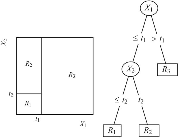
Decision trees describe partitions of the covariate space that maximize differences in the outcome. Right: A decision tree describing partitions of the covariates X₁ and X₂ into the areas R₁, R₂, and R₃. In this example, covariate X₁ was split at value t₁, and a subsequent split of covariate X₂ at value t₂ was found in the left subtree. Left: A two-dimensional plot of the partitioned covariate space in the areas R ₁, R ₂, and R₃.

Structural Equation Model Trees

Model-based trees enhance the decision tree paradigm by partitioning the data set with respect to differences prescribed by a hypothesized model. Thus far, model-based trees focused on differences in model parameters describing relations between observed variables. SEM Trees extend these approaches to a target structure that is specified at the latent level. Due to the great flexibility of SEM, SEM Trees facilitate exploratory analyses for a large range of models, including regression models, factor analytic models (Jöreskog, 1969), autoregressive models (Jöreskog, 1970), latent growth curve models (McArdle & Epstein, 1987), latent difference score models (McArdle & Hamagami, 2001), or latent differential equations (Boker, Neale, & Rausch, 2004). Typical questions that can be addressed with SEM Trees include the following: “Is there a significant difference in the mean values of a latent construct in subpopulations of the data set with respect to the covariates?” or “Does the correlation between a latent intercept and a latent slope in a latent growth curve model differ between specific subgroups of a population?”

To find and interpret differences between individuals or groups in factor-analytic models, measurement invariance has to be ensured (Meredith, 1993), that is, restrictions of freely estimated parameters have to be established across groups. SEM Trees include specific mechanisms to guarantee measurement invariance and can thus provide insight whether the chosen level and type of invariance holds across a data set for a given factor model. On the other hand, finding significant differences in this framework without the invariance assumption is also possible. The latter property of SEM Trees enables the retrieval of different factor profiles for distinct sub-populations.

In an exploratory data analysis, researchers might choose to sequentially include covariates in models to examine their influences on model variables. Alternatively, models are sometimes split into multi-group models according to covariates, such as age or sex, sometimes with the hope to identify homogeneous sub-groups for which the hypothesized model fits better. For example, Asparouhov and Muthén (2009) set up a two-group model by participants’ sex and, in a second step, expanded this model by adding a poverty index as latent predictor. Such kinds of model selection processes are often driven by more or less implicit heuristics and proceed in an exploratory or quasi-exploratory fashion. For example, in developmental research on age differences in cognition, the selection of age groups is informed by prior knowledge about the age trajectories of task-relevant mechanisms (e.g., Kray & Lindenberger, 2000). Although sample and variable selection can be effective in practice, it generally lacks a formal justification. In particular, the selection process is susceptible to implicit or explicit biases of the investigator (cf. Kriegeskorte, Simmons, Bellgowan, & Baker, 2009).

Whenever models are built from a single data set, there is the danger that the model will fit the data set well but will generalize poorly to others. This is called overfitting the data. Some practices in SEM, such as the use of modification indices and some fit indices, mislead the researcher in engaging in an exploratory model selection process while reporting confirmatory statistics. Sometimes, this is referred to as data dredging or capitalizing from chance. SEM Trees are built around a greedy selection procedure that builds tree structures based on criteria that account for the dangers of overfitting and allow to find generalizable features in the data.

SEM Trees offer a formal setting for model selection by combining confirmatory and exploratory approaches. Main influences and interactions of covariates on the parameter estimates of a template model are found in an exploratory fashion, while theory-based assumptions and hypotheses can be represented in the SEM. SEM Trees then allow in a successive step to confirm the refined hypothesis on an evaluation set of participants. The importance of such an evaluation has been stressed repeatedly in the modeling literature (Bishop, 2006; Browne & Cudeck, 1992; Kriegeskorte et al., 2009).

Techniques for recursive partitioning of SEM have also been suggested by Merkle and Zeileis (2011) and Sanchez (2009). Both approaches are implemented in R packages. The former is available as strucchange by Zeileis, Leisch, Hornik, and Kleiber (2002), and the latter is available as pathmox by Sanchez and Aluja (2012). Strucchange can be employed for a recursive partitioning methodology based on a generalized fluctuation test framework, whereas the pathmox software provides recursive partitioning of path models based on partial least squares estimation. Differences between pathmox and SEM Trees primarily reflect differences of the underlying estimation techniques, which is least squares for pathmox and maximum likelihood for SEM Trees. For a comparison of those, see Jöreskog and Wold (1982).

In the remainder of this article, we formally define SEM Trees and discuss two methods to evaluate covariate-specific splits of a given data set during the tree growing process, one based on a Bonferroni-corrected likelihood ratio test and the other on crossvalidation estimates. We explain how measurement invariance is implemented in SEM Trees, thereby greatly facilitating the use of factor analytic models. We also discuss ways to incorporate parameter restrictions across a tree structure, and we discuss possibilities to apply pruning, a technique designed to increase the generalizability of tree structured models. To illustrate the utility of SEM Trees in exploratory data analysis, we present SEM Tree analyses of previously published empirical data sets using a latent growth curve model and a standard factor model. We conclude by detailing some strengths and limitations of the SEM Tree framework.

Structural Equation Modeling

SEM Trees can be conceived as a hierarchical structure of models, in which each model is a SEM. In structural equation modeling, models are constructed by specifying a model-based expectations vector µ and a model-based covariance matrix l. By imposing or freeing restrictions in these matrices, different concepts and hypotheses about the data can be integrated into a single model. The key feature lies in the comparison of the model-based expectations and covariances with the observed expectations and covariances in a data set. Based on a discrepancy function, model parameters can be estimated, and indices of goodness-of-fit can be derived.

SEMs have been extensively discussed in the literature. For an introduction, see for example the textbook by Bollen (1989). SEMs constitute a widely applied multivariate analysis technique and can be seen as a unification of several multivariate statistics (cf. Fan, 1997). Different representations of SEMs proposed in the literature, among which LISREL (Jöreskog & Sörbom, 1996) and RAM (Boker, McArdle, & Neale, 2002; McArdle & Boker, 1990; McArdle & McDonald, 1984), can be used for SEM Trees. A diverse range of methods exists for parameter estimation in SEM, that is, least squares, partial least squares, maximum likelihood, and expectation maximization. Under the assumption of multivariate normality, maximum likelihood estimation has some convenient properties, such as the availability of standard errors of the parameter estimates, known distributional properties of the test statistic, and efficiency of the estimator.

With the full information maximum likelihood (FIML) formulation, robust parameter estimation under missing data is feasible (Finkbeiner, 1979). For notational convenience, twice the negative log-likelihood (−2LL) usually replaces the likelihood function. The case-wise −2LL of the model under the data is obtained through the following equation:

$$-2L{L}_i=K_i+\log \mid {\Sigma }_i\mid +({\mathrm{x}}_i-{\mu }_i)\prime {\Sigma }_i^{-1}({\mathrm{x}}_i-{\mu }_i)$$ (1)

where K_i is a constant depending on the number of non-missing data points, Σ_i is the model-implied covariance matrix with rows and columns deleted according to the pattern of missingness in the ith observation x_i, and likewise µ_i is the model-implied meanvector with elements deleted according to the respective pattern of missingness.

Since the observations are assumed to be independent, the complete −2LL function for n independent observations is given by the following:

$$-2LL=\sum _{i=1}^n-2L{L}_i$$ (2)

Parameters are estimated by minimizing this function, usually by an iterative, gradient-based optimization method (e.g., von Oertzen, Ghisletta, & Lindenberger, 2009).

From Model to Tree

SEM Trees are a variant of model-based recursive partitioning. Instead of fitting a single model to an observed data set, the data set is partitioned with respect to covariates that explain the maximum difference in the parameter estimates of the hypothesized model. This partitioning procedure is applied in a hierarchical fashion as long as differences are discovered. For example, in a factor model, a SEM Tree could identify covariates, that is, measured variables describing subsets of the sample, that maximally differ in their latent mean score. In a bi-variate linear latent growth curve model, a SEM Tree could retrieve subgroups that maximally differ in their latent slope correlation. A SEM Tree can be depicted as a tree structure with each node in the tree representing a SEM. Each inner node of the tree also represents a split point with respect to a covariate. The respective child nodes are associated with a SEM that represents the induced subsamples of the data set.

For illustration, assume a data set of N = 400 participants of two age groups: “young” and “old.” Half of each group participated in a cognitive training program that is supposed to prevent or attenuate cognitive decline with age. The decline is assumed linear and thus is modeled with a linear latent growth curve model, which measures a hypothetical cognitive score on four occasions of measurement. Model parameters include mean µ and variance a² of the intercept and mean µ and variance a² of the slope. This hypothetical example is inspired by the literature on cognitive intervention in old age (for summaries, see Baltes, Lindenberger, & Staudinger, 2006).

Let us assume that decline in older adults was steeper than in younger adults, and that the treatment only affected older participants by reducing the slope of their decline process to the extent that it was similar to that of younger participants. In this instance, the SEM Tree would find the covariate interaction of “age” and “treatment.” Results for a simulated data set are shown in Figure 2. The SEM Tree split the data set according to age and recursively proceeded to split the older individuals into two subgroups that significantly differ in their growth curve parameters, namely those with the treatment and those without. The group of younger individuals was homogeneous with respect to the model parameters and was not selected for a further split. The simulated data set also contained a further covariate “noise,” which was generated from a Bernoulli process. In the process of growing the tree, this variable has never been selected because it has no explanatory power with respect to differences in the parameter estimates. While this setting is likely subject to a confirmatory analysis of variance, the strengths of SEM Trees come to the fore when (1) parameter specifications (e.g., error structure, latent factors) imply the need to set up a SEM, and (2) when the number of covariates is large, their interaction unknown, or both (e.g., sets of behavioral, cognitive, or genetic covariates).

Figure 2.

Left: Illustration of a structural equation model (SEM) Tree with a linear growth curve model as the template model. Right: Predicted mean trajectories with respect to the groups identified by the SEM Tree.

Formal Definition

A SEM Tree is a tuple (T, M, O), with T being a tree structure, and with M being a θ-parameterized structural equation model and a set of parameter estimates for each node τ given as $\Theta =\{{\theta }_{\tau }\mid \tau \in T\}$.

We denote the set of leaves of the tree—that is, nodes without successors—with L(T). The set of all inner nodes—that is, nodes that have successors—is denoted by I(T). The number of leaves and the number of inner nodes of a tree will be noted by the cardinalities of the respective sets, |L(T)| and |I(T)|. A subtree T= is a tree that contains as root any node of T, and also all successors of this node. Subtrees of T will be denoted as T ≤ T. A SEM Tree with two successors of every inner node—that is, a tree that at each node describes a bi-partition of the covariate space—is a binary SEM Tree.

The SEM M will in the following also be referred to as template model. Using a fit index f, typically a maximum likelihood index, a SEM Tree is constructed from a data set D represented by a n × (k + l) matrix of observations D, which consists of n observations, k observed variables, and l covariates not modeled in M. The observed data matrix used for parameter estimation in M is denoted as the submatrix D_k = D_1..n,1..k, and the matrix of covariates is denoted by D_l = D_{1..n,k + 1..k + l}. The covariates constitute the set of candidate split variables. Each SEM Tree possesses a mapping function t/J(T, d), which maps an observation d to a node of T. Essentially, the mapping function traverses the tree with respect to the covariates of an observation and thus matches the observed variables of an instance to a particular submodel of the tree. If a covariate encountered in the traversal process is missing, the traversal process finishes at that particular inner node instead of in a leaf node. In particular, this mechanism allows the formulation of a likelihood function of a SEM Tree M given the data D with potential missingness in the data set. Alternatively, a surrogate approach can be used to deal with missing values (cf. Hastie, Tibshirani, & Friedman, 2001).

The −2LL of a SEM Tree M is defined as the sum over the −2LLs of all node models:

$$-2LL=(T\mid \mathbf{D})=\sum _{d\in \mathrm{D}}-2LL(M\left({\theta }_{\Psi (T,d)}\right)\mid d)$$ (3)

In a SEM Tree, the likelihood of observing the data is maximal for the given tree structure, that is, each node model is associated with parameter estimates that represent the optimal solution with respect to the fit index f. Put differently, in the maximum likelihood setting, a SEM Tree has the maximum likelihood of having observed the data set given that particular tree structure. This can be achieved by maximizing the individual likelihood functions of the node models since the observations are independent and the node splits induce a non-overlapping partition of the data set.

SEM Trees are depicted as tree graphs with nodes and edges (see Figure 2). Inner nodes are drawn as ovals and represent splits of the data set with respect to a specific covariate. The node is labeled with the name of the covariate. If available, the p-value of the test statistic that was used for evaluating the split candidate is appended to the node label to reflect the confidence in the selection of the respective node as covariate split. Leaves of the tree represent the estimated parameter sets for the subset of the data according to the performed partition of the original data set. Leaf nodes are represented as rectangles containing information about the estimation of the submodel, usually including the number of data points N that remained in the respective partition and all parameter estimates and, if required, estimates of their standard error and statistical significance of differing from zero.

Categorical, Ordinal, and Continuous Covariates

Initially, tree-based methods were created for dichotomous attributes. A generalization to categorical, ordinal, and continuous variables is realized with a dichotomization procedure of the variables under investigation (Quinlan, 1993). Categorical variables can be split into a set of dichotomous variables applying a one-against-the-rest scheme or by consideration of all possible non-empty dichotomizations. For example, if there are five categories of occupation, there are 15 possible splits. Hence, the computational needs are generally much heavier for categorical variables. Alternatively, it is possible to allow multiple splits into several subgroups according to the number of categories of a variable. In the latter case, the degrees of freedoms of the likelihood ratio test for split candidate evaluation have to be adapted accordingly. For ordinally scaled and continuous variables, we apply the dichotomization as suggested by Quinlan (1993), which is also known as exhaustive split search in the literature. At first, the data set is ordered according to the attribute A under consideration. Given the sorted values of A as v₁ … . v_m, this results in a maximum of m - 1 splits, the ith split being at (v_i + v_{i + 1})/2. Along the same line, nominal data with m categories can be split into 2^m-1 - 1 dichotomous split variables.

If a covariate that has been dichotomized in this way occurs repeatedly in a tree, the corresponding subset of participants has to satisfy both constraints. For example, if a split is “age below 50” and later on in that subtree, a split is “age above 25,” then the resulting subset of participants ranges in age between 25 and 50.

Particularly interesting is the fact that monotonic transformations of the covariates do not change the structure of the SEM Tree. In a regression model, a researcher might choose to model relations on a logarithmic scale. However, the non-linear interactions that are investigated in the covariate structure do not have to be log-transformed because this transformation does not affect the partitioning of the data set. In aging research, researchers sometimes choose to standardize variables, such as age in years, by subtracting the mean and dividing by the standard deviation or by using polynomial forms of the variable, such as age squared. Assuming that age is always positive, these transformations also are monotonic and are subsumed in the exploratory procedure of searching for possible attribute splits. Thus, they do not have to be explicitly specified.

In the following and in line with Zeileis et al. (2008), we restrict our considerations to binary SEM Trees. This imposes no loss of generality because an N-ary split of a single covariate can be represented by a sequence of N - 1 binary splits. Non-dichotomous covariates will be transformed to a set of dichotomous variables. The emerging set of original dichotomous and transformed dichotomous covariates forms the candidate pool for potential node splits during tree growing. This set is referred to as the set of implied covariates.

Algorithm

The following section describes the general procedure for growing SEM Trees.

General recursive partitioning

The generic split procedure for model-based recursive partitioning is simple:

1. Fit a parametric template model to the current data set via a chosen optimization procedure;

2. for each covariate, split the data set with respect to the covariate and compare the fit of the compound model of all submodels against the fit of the template model; and

3. choose among the compound models the one that is the best description of the data set according to a chosen criterion. If this model fits significantly better than the template model, repeat the procedure with Step 1 for all submodels. Otherwise terminate.

Given that the statistics for growing SEM Trees rely on asymptotic assumptions, it might be convenient to define a minimum number of observations min_N that is required for a node candidate to be considered legitimate. Nodes with a smaller number of observations will be skipped in node evaluation.

Growing SEM Trees

To put this generic algorithm into a SEM context, we operationalize the three steps listed above as follows. The parameterized model in our context is represented by any generic SEM, reflecting assumptions and prior hypotheses about the structure of the data. In our implementation, optimization is performed using a maximum-likelihood estimation procedure. However, the suggested approach does not rely on this particular estimation method. Any other discrepancy function can also be used for parameter estimation, such as generalized least squares or asymptotic distribution free methods. As long as the function provides an asymptotic x² fit-statistic, the procedures described in this article remain unchanged.

Since the compound model, which is a model subsuming all models generated by the covariate split, and the base model are nested, we can apply a likelihood ratio test to evaluate whether the model can be split into submodels. Indeed, the full model can be interpreted as the compound model with additional linear constraints of parameter equality across all submodels. Thus, evaluating a model split can be interpreted as comparing a multi-group SEM whose groups are determined by the levels of a covariate against a unitary model (i.e., a SEM Tree with only the root node).

The formal evaluation of a node split with respect to a selected covariate is explained in the following. For a given template model M, we are equipped with the likelihood function f(θ|D) for a parameter set θ with m free parameters and a data set D. We obtain the parameter set θ_F for the full data set by minimizing f(θ_F|D). For a given candidate split variable, assume a partitioning of the data set D into independent subsets D₁,…, D_k. Because the subsets are non-overlapping, the parameters θ₁, … , θ_k are found by independently minimizing f(θ₁|D₁), … , f(θ_k|D_k). The compound model of all submodels is from now on referred to as M_SUB. M is nested within M_SUB since M corresponds to M_SUB with n additional linear equality constraints on the free parameters in θ. Given the nested structure, we can formulate a null hypothesis that the model fit of M is not significantly different from M_SUB so that the parameters of the submodels are indeed the same, that is, H₀ : θ₁ = θ₂. The log likelihood ratio A between M and M_SUB is then given as

$$\Lambda =\sum _{i=0}^{k}LL({\widehat{\theta }}_i\mid {\mathbf{D}}_i)-LL({\widehat{\theta }}_F\mid {\mathbf{D}}_F)$$ (4)

Following Wilks’s (1938) theorem, A is x²-distributed with (k - 1)m degrees of freedom. Given a set of covariates, all possible splits are evaluated, and the model with the best increase in fitness is compared against a previously chosen threshold, determined by ex, the chosen probability of Type I error. If the split is statistically significant, splitting is continued recursively.

Multiple testing

The variable selection criterion based on the likelihood ratio test chooses the split candidate with the maximum increase in likelihood after splitting, and thus bases acceptance of a candidate variable on the known distribution of the individual test statistics under the null hypothesis. However, this selection strategy is plagued by a popular fallacy. In fact, by choosing the maximum of a set of statistics (one for each covariate to be tested), the resulting distribution is no longer the same as the distribution of the individual statistics. A typical solution to this situation is a conservative correction of the significance level of the likelihood ratio test, commonly known as Bonferroni correction. Under the assumption of independence of the individual tests, it corrects the maximally chosen test statistic such that the originally chosen ex level is valid. Since covariates are typically correlated to some degree, the Bonferroni correction is overly conservative. Several authors (Jensen & Cohen, 2000; Kriegeskorte et al., 2009) recommend cross-validation (CV) as an appropriate technique to estimate the generalization performance of a selection algorithm. In SEM Trees, CV can be employed for the node selection process. Instead of evaluating attribute candidates on the full data set S, n-fold CV will split the training into set into n disjoint sets S_i. For each candidate attribute split, the respective submodels will be created, and their SEM parameters will be estimated from S after the removal of S_i. The likelihood ratio for this particular partition of the training will be approximated by estimating the log-likelihood ratio of the implied node split on the remaining validation set S_i. The overall estimate of the log likelihood ratio test statistic for the candidate split is the average of the n estimates. Kohavi (1995) evaluated the choice of cross-validation for model evaluation in the context of univariate categorical outcomes with the C4.5 decision tree algorithm. His results suggest that a choice of 5- or 10-fold CV can be an appropriate choice for SEM Trees. Nevertheless, the effect of the number of folds on bias and variance of the estimator remains to be investigated more fully. The number of folds n is a crucial choice. In each CV iteration, parameters will be estimated from (n - 1)/n of the sample, and the test statistic will be evaluated on 1/n of the sample. Choosing a larger n will stabilize the parameter estimation process with only a small decrease in sample size. On the other hand, computation time linearly increases with larger choices of n. Generally, CV estimates for attribute selection only imply a moderate increase in computation time and will correct for the multiple comparison problem. When using CV, the likelihood ratio estimate no longer follows a x²-distribution because the parameter estimates cannot be assumed to be close to the optimum of the fit index for the holdout set. Therefore, thresholds for significant results cannot be chosen based on known distributions but only heuristically. The threshold we suggest is to accept the split whenever the CV estimator of the likelihood ratio is larger than zero, as in these cases the candidate split model represents the data on average better than the unitary model. More precisely, the expected likelihood of observing a new data point under the tree is larger than under the unitary model. The larger the estimate, the better the representation relative to the unitary model. Given the shortcomings of the Bonferroni-correction, we recommend using CV-based SEM Trees over Bonferroni-based SEM Trees. Nevertheless, we like to emphasize that researchers can in principle build trees of arbitrary depth without stopping rule and this procedure might help them to gain a better understanding of their data. Trees hold the ex-level of the statistical test employed for variable selection because hypotheses in a tree are recursively nested Zeileis et al. (2008).

Selection bias

Any tree-structured algorithm carrying out an exhaustive search in the split attribute space exhibits the problem of selection bias, sometimes also referred to as attribute selection error (Jensen & Cohen, 2000). With a growing number of possible splits in a variable, this variable is increasingly likely to be selected as a split criterion, solely based on the larger number of partitions of random fluctuations, which induce apparently significant results but merely reflect random noise. General principles to address variable selection bias were described by Jensen and Cohen (2000). In the context of decision trees, variable selection bias was addressed by different approaches. Two general approaches to reduce bias are (a) the selection of variables based on p-values instead of maximally selected test statistics, and (b) the separation of variable and split point selection (Shih, 2004). Frank and Witten (1998) computed p-values from permutation tests, and Dobra and Gehrke (2001) approximated p-values for the distribution of the GINI-index. QUEST (Loh & Shih, 1997) also bases the split-variable selection on p-values derived from an analysis of variance (ANOVA) F-statistic for ordered values or x²-statistic for categorical values and uses a Bonferroni correction to account for multiple testing across variables. The authors report that this procedure has negligible bias. CRUISE (Kim & Loh, 2001) is a variant that allows multiway splits. GUIDE (Loh, 2002) controls bias by relying on a chi-square analysis to detect interactions between the residuals and the covariates. Numerical variables are divided into four groups corresponding to sample quartiles. Hothorn, Hornik, and Zeileis (2006) proposed a generalized framework based on conditional inference procedures that provides unbiased formal tests for variable selection and stopping criteria. Zeileis et al. (2008) suggested a unified framework for unbiased model-based recursive partitioning that is based on tests for parameter instability. Strobl, Wickelmaier, and Zeileis (2011) presented an application of this framework on Bradley–Terry models. They used a two-stage procedure that first selects a variable by parameter instability test statistics and then selects the optimal cut point by maximizing the likelihood after the split. Using either the Bonferroni-correction or CV is subject to variable selection bias. One might be tempted to apply a nested Bonferroni-correction that corrects at the tree level for the number of candidates and at the variable level for the number of implied splits. However, this correction reverses the bias because variables with many levels are more severely penalized. A fair selection strategy can be achieved by following the advice of Shih (2004) and separating variable and split point selection. In order to illustrate the effects of selection bias in SEM Trees, we show some simulation results in Figure 3. In the simulation, trees were built from uninformative ordinal variables with different numbers of levels (2, 4, and 10). For three different selection strategies, the bars indicate how often the particular variable would have been selected as the best splitting variable. Since all three variables are generated to be uninformative, a fair selection strategy is expected to show a uniform distribution. As expected, a naive selection scheme, in this case a Bonferroni-correction, prefers variables with more levels under the null hypothesis that the variable is uninformative. A nested Bonferroni scheme reverses the bias by overly penalizing variables with many levels. In contrast, a two-stage procedure related to the ones implemented by Loh and Shih (1997) and Kim and Loh (2001), which first selects the best cut point for each variable and then selects among the best candidates, has negligible selection bias. This procedure can be used with both a Bonferroni-correction or cross-validation to correct for multiple testing at the level of the original covariates.

Figure 3.

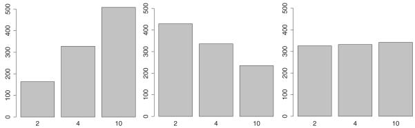
An illustration of variable selection bias for three different variable selection criteria: Bonferroni-correction (left), nested Bonferroni-correction (middle), and the fair selection criterion (right). Each subfigure depicts result of a simulation. The simulated data set contained three uninformative, categorical covariates with two, four, and 10 categories each. The depicted distribution shows the frequency with which each of these variables would have been picked under the null hypothesis. An unbiased variable selection algorithm is expected to have no preference for any variable.

Evaluation and pruning

The use of independent sets for model selection and model evaluation in data analysis has been emphasized in many contexts (Bishop, 2006; Browne & Cudeck, 1992; Kriegeskorte et al., 2009). If no independent sample is available, one usually divides the available data set into two disjoint sets: a training set and a test set. The training set is usually chosen to be larger than the test set to provide enough data for stabilizing the learning phase, that is, in the present case, the tree building phase. The test set can either be used for evaluation of the predictive performance of a tree or to prune back a tree to increase its generalizability. Pruning procedures select subtrees usually by pruning off terminal nodes by evaluating criteria that trade off reduction in heterogeneity against added complexity. An overview of different pruning algorithms can be found, for example, in Esposito, Malerba, Semeraro, and Kay (1997). One common pruning method for classification trees proposed by Quinlan (1987) is called Reduced Error Pruning. This technique can be straightforwardly employed with SEM Trees by replacing Quinlan’s classification error by the −2LL criterion. The algorithm prunes back terminal nodes of a SEM Tree as long as the −2LL of the test set improves. A different approach to pruning was suggested by Su et al. (2004), who proposed an Akaike information criterion (AIC)-based pruning strategy for trees based on models estimated with maximum likelihood procedures. An unbiased estimator of the generalization performance of a SEM Tree is the evaluation of an independent test set on the decision tree. For an independent data set, parameter estimates of the node models will not necessarily represent a maximum of the associated likelihood functions, and therefore the distribution of the likelihood ratios will be unknown. However, if the likelihood of having observed the test set is larger given the tree than given the root model only, we are inclined to believe that indeed the tree-implied model is a more appropriate representation of the population.

Computational Aspects

Asymptotic time complexity analysis

The run time of the algorithm depends on the sample size N and the number of dichotomous covariates M. For the evaluation of a potential new split, M calls to the SEM optimizer have to be made. The run time of the optimizer can be assumed to be linear in N if full information maximum likelihood (FIML) is employed. Bounds for the depth of the tree are the number of covariates M, and the binary logarithm of the number of cases log(N). In practical situations, most often we will find that log(N) < M. In that case, the run time will quadratically depend on the number of dichotomous covariates and linearly on the number of observations. When using k-fold CV for split evaluation, each parameter estimation process is executed k times, and therefore, the run time is linearly scaled by the number of folds. These considerations are general in the sense that they do not depend on a particular hardware or computing architecture.

Numerical parameter estimation

Parameter estimation in SEM requires the solution of an optimization problem. Typically, the solution is found by one of many numerical optimization methods. Given a set of starting values, the method will iteratively improve the estimate until the target function, such as the likelihood function value, will converge. In some cases, convergence is not reached, for example, if starting values are chosen far away from the unknown population values. Building a SEM Tree requires a large number of model fits and problems in some model fits are likely to occur.

The SEM Tree algorithm passes on parameter estimates of a node as starting values for submodels when evaluating splits. If the model does not converge, the original starting values can be used. If this still fails, either the potential split is disregarded or a new set of starting values has to be generated by a different estimation method, for instance, by a least-squares estimate. Non-converging models are marked during the tree growing process. Non-converging estimates can result for various reasons. Whenever non-converging models occur, the user is advised to cautiously inspect the reasons. If non-convergence occurs very early in the SEM Tree, model respecification is advised. In later stages of the growing process, non-convergence may reflect small sample size. In these cases, the limited information in the data set prevents the tree from being grown further. In our implementation, unique starting values and the passing-on of previous estimates as starting values is implemented.

Parameter restrictions

A particular strength of SEM is the possibility of algebraic restrictions on models. The likelihood ratio test offers statistical means to significantly reject restrictions if the sampled data contradict them. Most often, restrictions in SEM include either restricting a parameter to zero or restricting a set of parameters to be equal. Hence, significant values of the respective test statistics indicate that in the first case the parameter is truly different from zero or in the second case the chosen parameters are truly different from each other. Restrictions on SEM Trees help to test hypotheses, reflecting the substantive questions of the researcher.

In the following paragraph, we introduce two types of restrictions across models in a tree: (1) A global restriction requires a parameter from the template model to be the same across all models in the tree. Due to the greedy nature of the algorithm, this can be achieved only if values for the chosen parameters are estimated once on the full data set and regarded as fixed for all subsequent models. (2) A local restriction requires a parameter to be equal on all models whose nodes have the same father node only during split evaluation. This can be thought of as a parameter equality restriction across models in a multi-group setting. This leads eventually to diverging values of the restricted parameter in the leaf models. However, this restriction allows that parameters are freely estimated while their differences across submodels do not contribute to the evaluation of the split criterion. For example, in a regression model, a researcher might be interested in model differences with respect to the regression parameters, but not in differences of the regression line with respect to prediction accuracy, that is, the residual error term. In that case, the residual error can be defined as locally restricted. Without this restriction, the tree can in principle find distinct subgroups that are characterized by the exact same regression slope but differ only in the residual error term. Certainly, the latter case might also be of interest, depending on the researcher’s questions.

Variable Splits Under Invariance Assumptions

A widely used class of SEM are factor models that define relations between hypothesized latent factors and observed scores. In applied psychological research, hypotheses about factor-analytic structures are often tested across multiple groups. For example, in aging research, a common approach is the separation of the participants into models according to their age group, that is, a model for the younger and a model for the older participants (e.g., Kray & Lindenberger, 2000). Multi-group factor models are essentially represented by replications of a template model for each group whereby free parameters are unique within each group. Parameter constraints cannot only be set within groups but also across groups. This allows testing hypotheses whether parts of the model are indeed equal across groups or significantly differ from each other. An obvious question could be, “Do two groups differ in their average value of the latent construct?” These questions can be answered validly to the extent that the researcher can ascertain that latent constructs have been measured identically across all groups. This requirement, referred to as measurement invariance (MI) or measurement equivalence, has been debated in psychology for more than a century (Horn & McArdle, 1992; Meredith, 1964, 1993). Measurement invariance is traditionally tested through a sequence of hypothesis tests. While the literature has many concepts of invariance, most often four nested concepts are used: (1) configural invariance, sometimes termed configuration invariance or pattern invariance, requires the invariance of the pattern of zero and non-zero factor loadings across groups; (2) metric invariance, weak invariance, or factor pattern invariance requires invariance of the values of the factor loadings across groups; (3) strong invariance or scalar invariance assumes intercepts of the indicators and all factor loadings to be the same across groups; (4) strict invariance additionally restricts the residual errors to be equal across groups, to allow the interpretation of standardized coefficients across groups.

Having factor loadings, means, and variances all freely estimated could result in SEM Trees whose implied hierarchical group structure might violate the requested invariance qualifications. However, we definitely can gain knowledge about our data set from freely estimating all parameters. This would correspond to an exploratory search predicting the maximal difference between submodels and therefore subsumes covariates that maximally break the invariance assumptions. In line with Meredith (1993), we are inclined to require strong invariance whenever we are interested in latent mean differences. Since factor loadings express the expected change in the observed variable per unit of change of the latent variable, this invariance test is a test of equal scaling across the groups (Jöreskog, 1969). In that case, we suggest to only explore variable splits under the constraint that factor loadings are equal across all submodels. Effectively, the SEM Tree can be generated under the assumption of the chosen level of measurement invariance. By choosing a global restriction across the factor loadings, metric invariance can be imposed on the model; by extending the restriction to the score means, strong invariance is imposed. However, the assumption of MI is not yet statistically validated. By introducing additional tests whether these global restrictions hold at the stage of covariate split evaluation, the tenability of MI is ensured. Precisely, at each evaluation of a possible split in a submodel, a third model is introduced which is a variant of the submodel, only that the global restriction over the factor loadings is relaxed. The likelihood ratio between the compound submodel and the relaxed submodel allows testing MI in the traditional way by tentatively accepting the model as invariant if the null hypothesis cannot be rejected. Formally, let the estimated parameters of the full model before a split be θ_full, and the constrained compound split model’s parameters θ_res, and θ_free the freely estimated parameters of the compound model of all split models. These models are nested and their likelihood values will satisfy

$$-2LL\left({\theta }_{free}\right)<-2LL\left({\theta }_{res}\right)<-2LL\left({\theta }_{full}\right)$$ (5)

The only way to maintain a variable split is if the likelihood ratio 2LL(θ_full)−2LL(θ_res) is significantly different from zero, suggesting that the full model is truly a worse representation of the data set, and 2LL(θ_res)−2LL(θ_free) is not significantly different from zero, suggesting that the invariance assumption is tenable.

With this procedure in place, SEM Trees allow the generation of hierarchical model structures that predict parameter differences in SEM under a chosen assumption of measurement invariance, be it configural, metric, strong, or strict invariance.

Note that for factor-analytic models, both generative modes of the SEM Tree, either with or without measurement invariance, can make sense, depending on the researcher’s questions. A SEM Tree under measurement invariance can be used to predict differences in the factors, a regular SEM Tree might detect profiles of factor loadings that differ in the sample.

SEM Tree Package

We have implemented SEM Trees in the package semtree for the statistical programming language R (Ihaka & Gentleman, 1996), which is published as a complement to this article. It can be freely downloaded at http://www.brandmaier.de/semtree. The package is based on OpenMx (Boker et al., 2010), freely available at http://openmx.psyc.virginia.edu. In OpenMx, models can be specified with great flexibility, either in a matrix-based fashion or in a path-analytic way. Different representations of SEM proposed in the literature, among these LISREL (Jöreskog & Sörbom, 1996) and RAM (Boker et al., 2002; McArdle & Boker, 1990; McArdle & McDonald, 1984), can be used for SEM Trees. In particular, existing RAM-based OpenMx models can be run with the SEM Tree algorithm without modifications. The SEM Tree package provides methods for tree growing, pruning, evaluation, and plotting. Tree growing can be based either on the presented Bonferroni correction of the likelihood ratio test or on CV estimates. The latter is the recommended method. Local and global restrictions can be separately specified and the presented tests for MI are included. Tree pruning based on the reduced-error-pruning method is also implemented. All examples in this article were analyzed with this package. We also included facilities for tree visualization, both on-screen and as publication-ready LaTeX code.

Applications

To illustrate the utility of SEM Trees in data analysis, we present SEM Tree analyses on simulated and previously published empirical data sets. The examples include SEM Trees with four different template models, an autoregression model, a regression model, a longitudinal growth curve model, and a standard factor model.

Developmental Latent Growth Curves

McArdle and Epstein (1987) described aspects of latent growth curve modeling with a longitudinal data set of scores of N = 204 young children from the Wechsler Intelligence Scale for Children (WISC; Wechsler, 1949) over four repeated occasions of measurement, at about 6 years of age (t = 1), 7 years of age (t = 2), 9 years of age (t = 3), and finally at about 11 years of age (t = 4). Intellectual capability was measured on two distinct scales, representing verbal IQ and performance IQ. In line with McArdle and Epstein, we chose four subscales from each scale. The eight subscales included the Information, Comprehension, Similarities, Vocabulary, Picture Completion, Block Design, Picture Arrangement, and Object Assembly tests. The raw scores were rescaled to represent a “percent correct” scaling, thus ranging between 0 and 100. These were collapsed into an average score, which was investigated in further analyses. Covariates in the data set included the dichotomous variable sex, the continuous variable age at first measurement, and years of education of both mother and father in a categorical representation. Education of the father was the only variable that had missing values reported. The set of implied covariates had a size of 28.

We set up an equivalent factor model for an analysis with SEM Trees based on the data as described by Ferrer, Hamagami, and McArdle (2004) and McArdle and Epstein (1987). The template model for the SEM Tree was a linear latent growth curve model with a latent intercept and a latent slope, modeling a composite average score of the verbal and performance subscale over four occasions of measurement, with slope factor loadings λ₁ = 0, λ₂ = 1, λ₃ = 3 and λ₄ = 5 accounting for non-equidistant measurement occasions. The model was defined by six free parameters, mean µ_S and variance ${\sigma }_S^2$ of the slope, mean µ_I and variance ${\sigma }_I^2$ of the intercept, ${\sigma }_e^2$ for the measurement error, and ${\sigma }_{SI}^2$ for the correlation between intercept and slope.

A SEM Tree was generated from the full data set. Model differences were investigated with respect to the set of all six free parameters. We constructed trees both with the Bonferroni correction (ex= .05) and with CV estimates with a required minimum of min_N = 20 observations per leaf. The resulting from applying CV was in fact a pruned subtree of the Bonferroni-constructed SEM Tree. In Figure 4, the SEM Tree with the p-values from the Bonferroni-corrected construction method is presented. According to the CV method, the left subtree was associated with a significant improvement in model fit. Both construction methods found the variable mother’s education as primary split and found a subsequent split according to father’s education in the right subtree. The right subtree with the split point sex was not chosen by CV and would not have been chosen with the Bonferroni-corrected method with an ex-level of .01. This suggests that this split should indeed be ignored.

Figure 4.

Upper panel: Structural equation model (SEM) Tree on the longitudinal Wechsler Intelligence Scale for Children data set. A linear latent growth curve model served as the template model. The model indicates that the sample is maximally heterogeneous with respect to mother’s education, which accounts for differences in the learning curves between the two subsamples. The split point of both father’s and mother’s education corresponds to whether they graduated from high school. The dashed line indicates the subtree that was not constructed when cross-validation was used as the construction method. Lower panel: Representation of the linear latent growth model that served as the template model for the SEM Tree above.

In their original analysis of the data, McArdle and Epstein (1987) also reported that mother’s education predicted differences in children’s cognitive growth, which, they claim, would have been overlooked by individual path analysis or multivariate analysis of variance (MANOVA) models. While the influence of mother’s education on the model was a priori selected to be explored, the SEM Tree included an entire set of covariates and found mother’s education to predict the largest differences with respect to the model parameters.

The parents’ education covariates were originally coded with six categories, the first three representing various levels of high school graduation and graduation from schools beyond high school, and three levels for pre-high school education. Remarkably, the algorithm mimicked this plausible distinction of both education covariates in a purely data-driven fashion by separating children according to whether their mothers and fathers graduated from high school.

To examine the stability of the algorithm in the context of this data set, we drew 100 bootstrap samples. In each replication, we drew N = 204 samples from the original data with replacement to construct a training set. The remaining samples formed an independent test set. SEM Trees were generated from the training sets like described above and were evaluated on the test sets. In all 100 out of 100 replications, the SEM Tree algorithm found a model description, according to which the SEM Tree model with splits was more likely to be true than the unitary growth curve model. In 33 out of 100 of the bootstrapped trees, mother’s education was chosen as first split variable. In all these trees, “father’s education” was chosen as a single further split, thus replicating the tree structure obtained from the whole sample. In the remaining 67 bootstrapped trees, “father’s education” was chosen as first split variable. Interestingly, in only two out of these 67 trees, “mother’s education” was chosen as a subsequent split. The variables sex and age were never chosen. These results indicate that both parents’ education variables predict key differences in the model parameters. Particularly, father’s education seems a strong predictor (chosen in total in 98 of 100 replications). The possibility to get either mother’s or father’s education as first split is not surprising considering their high correlation in the population.

Factor Analysis of Wechsler Adult Intelligence Scale—Revised (WAIS–R; Wechsler, 1981) Data

The WAIS–R contains performance scores on eight subscales, similar to the WISC data set described in the previous section. We base our analysis on a data set that was previously analyzed by others, that is, McArdle and Prescott (1992) and Horn and McArdle (1992). The sample was collected during 1976 and 1980 by the Psychological Corporation and includes the scores of N = 1,880 individuals on a total of 11 WAIS–R subscales. A rich set of demographic covariates is available for this data set, including age group (in nine categories, hence eight implied dichotomous covariates), geographical information about the place of residence (four nominal categories, hence seven implied covariates), urban/rural place of residence (dichotomous), place of birth in the United States (dichotomous), marital status (again four nominal categories, hence seven covariates), handedness (dichotomous), education (six ordinal categories, hence five covariates), occupation (six nominal categories, hence 31 covariates), sex (dichotomous), and birth order (nine ordinal categories, hence eight covariates). In total, these resulted in 70 dichotomous variables.

Following McArdle and Prescott (1992), we included all individuals 18 years of age or older, obtaining a sample size of N = 1,680. For a first evaluation, we set up a single factor model that hypothesizes a latent factor representing verbal IQ on four verbal performance scores, represented by a latent mean µ_IQ and a latent variance ${\sigma }_{IQ}^2$. The performance on the remaining seven WAIS–R subscales was not considered in this example. The factor loading of the Information score (IN) was fixed at λ₁ = 1 and also the corresponding expectation of the observed score µ₁ = 0. Free parameters in the model include the remaining factor loadings λ₂ (Comprehension); λ₃ (Similarities); λ₄ (Vocabulary); and the residual errors ε₁, ε₂, ε₃, ε₄ of the four scores.

In the first run, the factor loadings were chosen to be tested for weak measurement invariance, that is, only candidate splits that fulfill this requirement were considered for further evaluation. The resulting SEM Tree under the factorial invariance assumption is shown in Figure 5 with a maximum depth of 4 to maintain readability for this form of presentation. Interestingly, the first two splits concern the levels of the education variable splitting off the two extreme groups from the data set, those with an education of 0 –7 years (education = 1) and those with an extremely long education of 16+ years (education = 6). For both extreme groups, there is no subsequent split that represents an improvement. For the remaining 1,335 individuals, occupation brought out the largest difference with respect to model parameters. The resulting two partitions were semi-skilled and skilled workers (occupation = 4, 5) versus all other occupations. For both subgroups, again, education described the largest difference, depending on whether participants had an education of more or less than 12 years (left subtree) or 13–15 years (right subtree). Thus, average differences in the latent expectation seemed monotonically related with the variable education. Another difference worth mentioning is the difference in the expectation of the Similarities score (µ₃) across groups determined by the variable occupation.

Figure 5.

Structural equation model (SEM) Tree with a factor model representing a single factor of verbal IQ, which was observed on four subscales from the Wechsler Adult Intelligence Scale—Revised data set for N = 1,680 individuals. The resulting splits indicate that the demographic covariates education and occupation account for substantial differences in the hypothesized model.

In a second run, we grew a tree without the invariance assumption to a maximum depth of 3. This analysis might guide us in finding potential splits in heterogeneous subgroups that are not invariant with respect to their factor loadings. Results might hint at splitting the data set with respect to one or more covariates into subgroups that are less easily compared with each other but might alert us to substantially meaningful differences in their factor structures. A resulting tree could be interpreted as covariate influences on different intelligence profiles, or more generally, sub-groups that systematically differ in the composition of the latent score. Subsequently, each of these models again can be analyzed with a second run of SEM Tree that incorporates the invariance assumption.

Figure 6 depicts the resulting tree without the invariance assumption, that is, each subtree features unique estimates for the loadings. The resulting tree resembles the tree under invariance to some extent. However, as the subgroups were allowed to differ in their factor loadings, the resulting estimates for the latent structure should be compared across models with caution. At the same time, the resulting tree can guide theory development by discovering meaningful differences in intelligence profiles.

Figure 6.

Structural equation model (SEM) Tree on the Wechsler Adult Intelligence Scale—Revised data set with a factor model as the template. The tree was generated in the default mode without implementing and testing invariance assumptions.

Limitations and Extensions

SEM Trees inherit the statistical properties that the template SEM and the chosen estimator impose; for example, when using a maximum likelihood estimator, multi-variate normality is an essential requirement. Also, since likelihood ratio tests are used to select the splits, the general properties and limitations of the likelihood ratio test in SEM apply to SEM Trees as well. Therefore, simulation results describing differential power of the test with respect to type of parameter, sample size (MacCallum, Widaman, Zhang, & Hong, 1999; Muthén & Curran, 1997), balance between groups (Hancock, 2001; Kaplan & George, 1995), incomplete data (Dolan, van der Sluis, & Grasman, 2005; Enders, 2001), non-normality (Enders, 2001), or model type—for example, latent growth curve model (Fan, 2003; Hertzog, von Oertzen, Ghisletta, & Lindenberger, 2008) or factor model (Hancock, 2001; Kaplan & George, 1995)—are directly pertinent to SEM Trees. In particular, this large body of research implies that differential power of the test can be critical for highly unbalanced subtrees (cf. Hancock, 2001; Kaplan & George, 1995). Furthermore, it is important to note that the power to detect group differences depends on the number and types of freely estimated parameters in the model. In future work, we plan to consider different estimators, which are, in some situations, more robust to violations of the normality assumption, like generalized least squares or weighted least squares (cf. Browne, 1974). SEM Trees provide a good basis for such extensions, as the choice of the objective function for the parameter estimation can be replaced without changes to the method for constructing the tree.

A second limitation coming from multi-group models is that sufficiently many participants have to be assigned to each group to ensure approximately asymptotic behavior. Multiple suggestions for an appropriate sample size have been made, ranging from minimum sample sizes of 10 –200 (cf. Tanaka, 1987). If groups are formed by few individuals only, standard errors of parameter estimates have to be interpreted with great caution. A possible way to decrease the influence of small sample size is to apply Bayesian estimation (cf. Lee, 2007), which we see as an interesting extension of SEM Trees.

The tree growing algorithm proceeds in a greedy fashion, that is, locally optimal choices are taken at each step of the growing process. The researcher has to keep in mind that the resulting tree is not necessarily the single best tree. Particularly, a tree can be susceptible to marginal changes in the data set, resulting in different choices for node splits and eventually structurally different trees. Building a set of trees from bootstrap samples sheds light on the stability of a tree (Strobl et al., 2009). A more rigorous approach is the generation of Structural Equation Forests, that is, ensembles of SEM Trees that were built from resampling the original data set. Breiman (2001) introduced random forests as ensembles of decision trees, and interesting measures of variable importance (cf. Strobl, Boulesteix, Zeileis, & Hothorn, 2007) exist that could be applied to SEM Forests straightforwardly. By using forests instead of trees, one moves from statistical modeling to algorithmic modeling and trades interpretability for stability (Berk, 2006) at the additional cost of computation time. An analysis with a forest can complement a single-tree analysis, of course.

Given the variety of solutions that arise from the selection of parameter estimation methods, split candidate selection methods, and hyper-parameters (e.g., folds in cross-validation), systematic methodological simulation studies are needed to comparatively evaluate the methods with respect to their performance in recovering known data structures. To enhance the use of SEM Trees in the toolbox of applied researchers, further simulations studies can help to outline problematic situations for the interpretation of tree structures in empirical research, including, for example, model misspecification, data perturbation, and violations of the normality assumption. Furthermore, future work needs to compare the different available tree-based estimation frameworks—such as SEM Trees, pathmox, and mob, strucchange—using both empirical and simulated data in terms of effectiveness and efficiency.

Discussion

Summary and Comparison to Other Approaches

By combining the benefits of exploratory and confirmatory approaches, SEM Trees provide a powerful tool for the theory-guided exploration of empirical data. The approach offers exploratory analyses for the refinement of a large range of hypothesized models. For models that require the assumption of measurement invariance, trees can be constructed in a way that only covariates are chosen that guarantee invariance across all tree-induced models. We discussed two methods to construct trees, based on distributional assumptions of the likelihood ratio test for candidate split evaluation and on cross-validation estimates of the likelihood ratio. In particular, we discussed selection bias and its remedy for naive selection strategies. In addition, we discussed how parameter constraints can be incorporated across node models. Also, we discussed a pruning method to increase generalizability of SEM Trees. Using two empirical examples based on previously published and analyzed data sets, we illustrated how SEM Trees can find substantially meaningful interactions of covariates and model parameters in different settings.

Instead of a single model for all participants, a multi-group model may often represent the structure of the data in a more appropriate way. In clinical trials, subgroup analysis is conducted to test whether a treatment affects subgroups of the sample differently. Here, SEM Trees can be regarded as a structured approach to recursive subgroup partitioning in relation to a set of covariates. In general, SEM Trees are similar to unsupervised clustering techniques in addressing the question whether latent variables and their relations among each other and to observed variables form covariate-specific clusters.

Main advantages of trees over classical statistical models are their potential to reveal non-continuous interactions and non-linear relations between covariates and outcomes. Also, SEM Trees make no assumptions about the distribution of covariates and are relatively insensitive to outliers (cf. Breiman et al., 1984). We expect trees to be particularly useful whenever there are many predictors with no clear indication which one should be considered first, whenever there is a large number of interactions whose nature is not known in advance, or both. Conversely, we expect trees to add little or nothing to other statistical tools whenever the number of covariates is small and the hypotheses are few and straightforward. Also, if the model generating the data is linear and additive, the tree may uncover an overly complex structure.

In the context of longitudinal data, SEM Trees are related to longitudinal recursive partitioning as introduced by Segal (1992), including the extension presented by Zhang and Singer (1999). Segal extended the decision tree paradigm to multivariate outcomes allowing the modeling of longitudinal data. As he points out, visual analysis is often performed to detect substantial differences in longitudinal analysis. However, this approach lacks a formal definition of difference and, relying only on the researcher’s experience, is prone to error. With large sample sizes, the identification of subgroups with structural differences quickly becomes unfeasible, and more complex relations between latent variables will tend to be hard to detect by visual inspection of observed variables alone. Therefore, a robust and systematic way of identifying and comparing substructures is crucial. SEM Trees extend Segal’s approach by offering a larger variety of underlying models and the ability of appropriately handling missing values.

A different exploratory technique, latent mixture modeling (McLachlan & Peel, 2000), has attracted interest in analyses based on SEM. In this framework, observations are assumed to come from a mixture of two or more unobserved distributions. Usually, this method requires determining the number of latent classes a priori, although McLachlan and Peel (2000) suggested that boot-strapping may be used to overcome this constraint. SEM Trees are designed to detect underlying homogeneous groups in the observations, but without a need to determine the number of latent classes a priori. While in latent class modeling the resulting classes may sometimes be difficult to interpret, the strength of SEM Trees is that the hierarchy of classes is based on covariates and will thus be interpretable.

An interesting question is whether the use of least squares, as employed in the pathmox R package, may show different convergence properties than the maximum likelihood driven approach of SEM Trees. Future work needs to compare the different estimation frameworks such as SEM Trees, pathmox, and strucchange, using both empirical and simulated data.

A future line of research is to integrate time-varying covariates into SEM Trees. SEM Trees are well suited for this extension, as the integration of time-varying covariates is common in SEM, but research needs to be done to find optimal ways of integrating these covariates into the split process.

SEM Trees: The Larger Picture

We would like to conclude this article by highlighting the utility of SEM Trees from two perspectives, one taken in the behavioral sciences, and the other taken in computer science. We take the abductive theory of scientific method (ATOM; Haig, 2005) as a typical representative of perspectives found in the behavioral sciences, and the framework of knowledge discovery in databases (KDD; Fayyad, Piatetsky-Shapiro, & Smyth, 1996) as a typical representative of the computer science approach.

Essentially, both approaches recognize and advocate that knowledge gain requires the recursive interplay of exploration and hypothesis testing. Stable patterns are extracted from data, which are called information in KDD and phenomena in ATOM. Then, knowledge is derived from information (KDD); respectively, theories are built from the phenomena (ATOM). SEM Trees add a tool that seeks to identify novel patterns in data; this property serves the function of extracting stable patterns from data. At the same time, they also provide visual and statistical indicators about extracted patterns; this property helps in theory building and may iteratively inform subsequent data extraction. By choosing an initial model, typically in a confirmatory setting, and by selecting interesting covariates, SEM Trees combine exploratory and confirmatory qualities.

Generally, we advise researchers to report results of a SEM Tree as exploratory. Two warnings are important: (1) SEM Trees do not provide a shortcut from data to theories or from data to knowledge but merely provide efficient tools reciprocally relating the two, and (2) as any new pattern from data mining must prove its utility with future data, each new theory must be evaluated on a new data set, ideally using a custom-tailored paradigm to test the hypothesized effects (cf. König, Malley, Weimar, Diener, & Ziegler, 2007).

In line with the propositions of ethical data analysis by McArdle (2010), we encourage researchers to first run their confirmatory analyses so that the use of their chosen statistical tests will be appropriate and valid. In subsequent steps, SEM Trees can offer a solid tool to refine these hypotheses. Also, SEM Trees avoid implicit selection bias of the investigator because there is no prior advantage of any covariate in the tree generation process.

When researchers have multiple competing hypotheses about their data, the hypotheses can be formalized in either the same SEM with varying restrictions, or in different classes of SEM. In principle, SEM Trees do not have to be limited to a single template model. Our on-going research involves hybrid SEM Trees that not only find differences with respect to parameters of the same model but allow for testing sets of hypothetical models against each other.

The process of growing SEM Trees involves multiple steps of data fitting, which can be time consuming. However, the algorithm allows naturally for a high degree of parallelization, as each subtree can be grown without interaction with the other subtrees.

To conclude, SEM Trees provide a versatile statistical tool that combines exploratory detection of influences of covariates on parameter estimates for latent variables, while at the same time offering formal confirmatory mechanisms to ensure generalizability. An implementation of SEM Trees with a range of options described in this article is available (Brandmaier, 2012) in R, based on the OpenMx package for SEM.

References

- Asparouhov T, Muthén B. Exploratory structural equation modeling. Structural Equation Modeling: A Multidisciplinary Journal. 2009;16:397–438. doi:10.1080/10705510903008204. [Google Scholar]
- Baltes P, Lindenberger U, Staudinger U. Lifespan theory in developmental psychology. In: Damon W, Lerner R, editors. Handbook of child psychology. Vol. 1. Wiley; New York, NY: 2006. pp. 569–664. [Google Scholar]
- Berk R. An introduction to ensemble methods for data analysis. Sociological Methods & Research. 2006;34:263–295. doi:10.1177/ 0049124105283119. [Google Scholar]
- Bishop C. Pattern recognition and machine learning. Vol. 4. Springer; New York, NY: 2006. [Google Scholar]
- Boker S, McArdle J, Neale M. An algorithm for the hierarchical organization of path diagrams and calculation of components of expected covariance. Structural Equation Modeling: A Multidisciplinary Journal. 2002;9:174–194. doi:10.1207/S15328007SEM0902_2. [Google Scholar]
- Boker S, Neale M, Maes H, Wilde M, Spiegel M, Brick TR, Fox J. OpenMx: Multipurpose software for statistical modeling [Computer software manual] 2010 Retrieved from http://openmx.psyc.virginia.edu.
- Boker S, Neale M, Rausch J. Latent differential equation modeling with multivariate multi-occasion indicators. In: van Montfort K, Oud J, Satorra A, editors. Recent developments on structural equation models: Theory and applications. Kluwer Academic; Dordrecht, the Netherlands: 2004. pp. 151–174. [Google Scholar]
- Bollen K. Structural equations with latent variables. Wiley; Oxford, England: 1989. [Google Scholar]
- Brandmaier AM. semtree: Recursive partitioning of structural equation models in R [Computer software manual] 2012 Available from http://www.brandmaier.de/semtree.
- Breiman L. Random forests. Machine Learning. 2001;45:5–32. doi: 10.1023/A:1010933404324. [Google Scholar]
- Breiman L, Friedman JH, Olshen RA, Stone CJ. Classification and regression trees. Wadsworth International; Belmont, CA: 1984. [Google Scholar]
- Browne M. Generalized least squares estimators in the analysis of covariance structures. South African Statistical Journal. 1974;8:1–24. [Google Scholar]
- Browne M, Cudeck R. Alternative ways of assessing model fit. Sociological Methods Research. 1992;21:230–258. doi:10.1177/0049124192021002005. [Google Scholar]
- Chan K, Loh W. LOTUS: An algorithm for building accurate and comprehensible logistic regression trees. Journal of Computational and Graphical Statistics. 2004;13:826–852. doi:10.1198/106186004X13064. [Google Scholar]
- Dobra A, Gehrke J. Bias correction in classification tree construction. Proceedings of the 18th International Conference on Machine Learning; San Francisco, CA: Morgan Kaufmann; 2001. pp. 90–97. [Google Scholar]
- Dolan C, van der Sluis S, Grasman R. A note on normal theory power calculation in SEM with data missing completely at random. Structural Equation Modeling: A Multidisciplinary Journal. 2005;12:245–262. doi:10.1207/s15328007sem1202_4. [Google Scholar]
- Enders CK. The impact of nonnormality on full information maximum-likelihood estimation for structural equation models with missing data. Psychological Methods. 2001;6:352–370. doi:10.1037/1082-989X.6.4.352. [PubMed] [Google Scholar]
- Esposito F, Malerba D, Semeraro G, Kay J. A comparative analysis of methods for pruning decision trees. IEEE Transactions on Pattern Analysis and Machine Intelligence. 1997;19:476–491. doi:10.1109/ 34.589207. [Google Scholar]
- Fan X. Canonical correlation analysis and structural equation modeling: What do they have in common? Structural Equation Modeling: A Multidisciplinary Journal. 1997;4:65–79. doi:10.1080/ 10705519709540060. [Google Scholar]
- Fan X. Power of latent growth modeling for detecting group differences in linear growth trajectory parameters. Structural Equation Modeling: A Multidisciplinary Journal. 2003;10:380–400. doi:10.1207/ S15328007SEM1003_3. [Google Scholar]
- Fayyad UM, Piatetsky-Shapiro G, Smyth P. The KDD process for extracting useful knowledge from volumes of data. Communications of the ACM. 1996;39:27–34. doi:10.1145/240455.240464. [Google Scholar]
- Ferrer E, Hamagami F, McArdle J. Modeling latent growth curves with incomplete data using different types of structural equation modeling and multilevel software. Structural Equation Modeling: A Multidisciplinary Journal. 2004;11:452–483. doi:10.1207/ s15328007sem1103_8. [Google Scholar]
- Finkbeiner C. Estimation for the multiple factor model when data are missing. Psychometrika. 1979;44:409–420. doi:10.1007/BF02296204. [Google Scholar]
- Frank E, Witten I. Using a permutation test for attribute selection in decision trees. Proceedings of the 15th International Conference on Machine Learning; Madison, WI: Morgan Kaufmann; 1998. pp. 152–160. [Google Scholar]
- Haig BD. An abductive theory of scientific method. Psychological Methods. 2005;10:371–388. doi: 10.1037/1082-989X.10.4.371. doi:10.1037/1082-989X.10.4.371. [DOI] [PubMed] [Google Scholar]
- Hancock G. Effect size, power, and sample size determination for structured means modeling and mimic approaches to between-groups hypothesis testing of means on a single latent construct. Psychometrika. 2001;66:373–388. doi:10.1007/BF02294440. [Google Scholar]
- Hastie T, Tibshirani R, Friedman J. Springer; New York, NY: 2001. The elements of statistical learning. [Google Scholar]
- Hertzog C, von Oertzen T, Ghisletta P, Lindenberger U. Evaluating the power of latent growth curve models to detect individual differences in change. Structural Equation Modeling: A Multidisciplinary Journal. 2008;15:541–563. doi:10.1080/10705510802338983. [Google Scholar]
- Horn JL, McArdle JJ. A practical and theoretical guide to measurement invariance in aging research. Experimental Aging Research. 1992;18:117–144. doi: 10.1080/03610739208253916. doi:10.1080/03610739208253916. [DOI] [PubMed] [Google Scholar]
- Hothorn T, Hornik K, Zeileis A. Unbiased recursive partitioning. Journal of Computational and Graphical Statistics. 2006;15:651–674. doi:10.1198/106186006X133933. [Google Scholar]
- Ihaka R, Gentleman R. R: A language for data analysis and graphics. Journal of Computational and Graphical Statistics. 1996;5:299–314. [Google Scholar]
- Jensen D, Cohen P. Multiple comparisons in induction algorithms. Machine Learning. 2000;38:309–338. doi:10.1023/A: 1007631014630. [Google Scholar]
- Jöreskog KG. A general approach to confirmatory maximum likelihood factor analysis. Psychometrika. 1969;34:183–202. doi:10.1007/ BF02289343. [Google Scholar]
- Jöreskog KG. Estimation and testing of simplex models. British Journal of Mathematical and Statistical Psychology. 1970;23:121–145. doi: 10.1111/j.2044-8317.1970.tb00439.x. [Google Scholar]
- Jöreskog KG, Sörbom D. LISREL 8 user’s reference guide [Computer software manual] Scientific Software; Milwaukee, WI: 1996. [Google Scholar]
- Jöreskog KG, Wold H. The ML and PLS techniques for modeling with latent variables: Historical and comparative aspects. Systems Under Indirect Observation: Causality, Structure, Prediction. 1982;1:263–270. [Google Scholar]
- Kaplan D, George R. A study of the power associated with testing factor mean differences under violations of factorial invariance. Structural Equation Modeling: A Multidisciplinary Journal. 1995;2:101–118. doi:10.1080/10705519509539999. [Google Scholar]
- Kim H, Loh W. Classification trees with unbiased multiway splits. Journal of the American Statistical Association. 2001;96:589–604. doi:10.1198/016214501753168271. [Google Scholar]
- Kohavi R. A study of cross-validation and bootstrap for accuracy estimation and model selection. In: Mellish C, editor. International Joint Conference on Artificial Intelligence. Vol. 14. Morgan Kaufmann; Los Altos, CA: 1995. pp. 1137–1145. [Google Scholar]
- König IR, Malley JD, Weimar C, Diener H-C, Ziegler A. Practical experiences on the necessity of external validation. Statistics in Medicine. 2007;26:5499–5511. doi: 10.1002/sim.3069. doi:10.1002/sim.3069. [DOI] [PubMed] [Google Scholar]
- Kray J, Lindenberger U. Adult age differences in task switching. Psychology and Aging. 2000;15:126–147. doi: 10.1037//0882-7974.15.1.126. doi:10.1037/0882-7974.15.1.126. [DOI] [PubMed] [Google Scholar]
- Kriegeskorte N, Simmons W, Bellgowan P, Baker C. Circular analysis in systems neuroscience: The dangers of double dipping. Nature Neuroscience. 2009;12:535–540. doi: 10.1038/nn.2303. doi:10.1038/nn.2303. [DOI] [PMC free article] [PubMed] [Google Scholar]
- Lee S. Structural equation modeling: A Bayesian approach. Wiley; New York, NY: 2007. doi:10.1002/9780470024737. [Google Scholar]
- Little T, Lindenberger U, Nesselroade J. On selecting indicators for multivariate measurement and modeling with latent variables: When “good” indicators are bad and “bad” indicators are good. Psychological Methods. 1999;4:192–211. doi:10.1037/1082-989X.4.2.192. [Google Scholar]
- Loh W. Regression trees with unbiased variable selection and interaction detection. Statistica Sinica. 2002;12:361–386. [Google Scholar]
- Loh W, Shih Y. Split selection methods for classification trees. Statistica Sinica. 1997;7:815–840. [Google Scholar]
- MacCallum R, Widaman K, Zhang S, Hong S. Sample size in factor analysis. Psychological Methods. 1999;4:84–99. doi:10.1037/1082-989X.4.1.84. [Google Scholar]
- McArdle JJ. Some ethical issues in factor analysis. In: Panter A, Sterber S, editors. Quantitative methodology viewed through an ethical lens. American Psychological Association Press; Washington, DC: 2010. pp. 313–339. [Google Scholar]
- McArdle JJ, Boker SM. RAMpath: A computer program for automatic path diagrams. Erlbaum; Hillsdale, NJ: 1990. [Google Scholar]
- McArdle JJ, Epstein D. Latent growth curves within developmental structural equation models. Child Development. 1987;58:110–133. doi:10.2307/1130295. [PubMed] [Google Scholar]
- McArdle JJ, Hamagami F. Collins LM, Sayer AG, editors. Latent difference score structural models for linear dynamic analyses with incomplete longitudinal data. New methods for the analysis of change. 2001:139–175. doi:10.1037/10409-005. [Google Scholar]
- McArdle JJ, McDonald RP. Some algebraic properties of the reticular action model for moment structures. British Journal of Mathematical and Statistical Psychology. 1984;37:234–251. doi: 10.1111/j.2044-8317.1984.tb00802.x. doi:10.1111/j.20448317.1984.tb00802.x. [DOI] [PubMed] [Google Scholar]
- McArdle JJ, Prescott CA. Age-based construct validation using structural equation modeling. Experimental Aging Research. 1992;18:87–115. doi: 10.1080/03610739208253915. doi:10.1080/03610739208253915. [DOI] [PubMed] [Google Scholar]
- McLachlan G, Peel D. Finite mixture models. Wiley; New York, NY: 2000. [Google Scholar]
- Meredith W. Notes on factorial invariance. Psychometrika. 1964;29:177–185. doi:10.1007/BF02289699. [Google Scholar]
- Meredith W. Measurement invariance, factor analysis and factorial invariance. Psychometrika. 1993;58:525–543. doi:10.1007/BF02294825. [Google Scholar]
- Merkle EC, Zeileis A. Generalized measurement invariance tests with application to factor analysis (Working Paper No. 2011-09) 2011 Apr; Retrieved from http://EconPapers.RePEc.org/RePEc:inn: wpaper:2011-09.
- Muthén B, Curran P. General longitudinal modeling of individual differences in experimental designs: A latent variable framework for analysis and power estimation. Psychological Methods. 1997;2:371–402. doi:10.1037/1082-989X.2.4.371. [Google Scholar]
- Quinlan J. Induction of decision trees. Machine Learning. 1986;1:81–106. doi:10.1007/BF00116251. [Google Scholar]
- Quinlan J. Simplifying decision trees. International Journal of Man-Machine Studies. 1987;27:221–234. doi:10.1016/S0020-7373(87) 80053-6. [Google Scholar]
- Quinlan J. C4.5: Programs for machine learning. Morgan Kaufmann; San Francisco, CA: 1993. [Google Scholar]
- Sanchez G. PATHMOX approach: Segmentation trees in partial least squares path modeling (Unpublished doctoral dissertation) Catalonia, Spain; Universitat Politecnica de Catalunya: 2009. [Google Scholar]
- Sanchez G, Aluja T. pathmox: Segmentation trees in partial least squares path modeling (R package Version 0.1-1) [Computer software manual] 2012 Available from http://CRAN.R-project.org/package=pathmox.
- Segal M. Tree-structured methods for longitudinal data. Journal of the American Statistical Association. 1992;87:407–418. doi:10.1080/01621459.1992.10475220. [Google Scholar]
- Shih Y. A note on split selection bias in classification trees. Computational Statistics and Data Analysis. 2004;45:457–466. doi:10.1016/ S0167-9473(03)00064-1. [Google Scholar]
- Sonquist J, Morgan J. The detection of interaction effects: A report on a computer program for the selection of optimal combinations of explanatory variables (No. 35) University of Michigan, Institute for Social Research, Survey Research Center; Ann Arbor: 1964. [Google Scholar]
- Spearman C. “General intelligence,” objectively determined and measured. The American Journal of Psychology. 1904;15:201–293. doi: 10.2307/1412107. [Google Scholar]
- Strobl C, Boulesteix A, Zeileis A, Hothorn T. Bias in random forest variable importance measures: Illustrations, sources and a solution. BMC Bioinformatics. 2007;8:25. doi: 10.1186/1471-2105-8-25. doi:10.1186/1471-2105-8-25. [DOI] [PMC free article] [PubMed] [Google Scholar]
- Strobl C, Malley J, Tutz G. An introduction to recursive partitioning: Rationale, application, and characteristics of classification and regression trees, bagging, and random forests. Psychological Methods. 2009;14:323–348. doi: 10.1037/a0016973. doi:10.1037/a0016973. [DOI] [PMC free article] [PubMed] [Google Scholar]
- Strobl C, Wickelmaier F, Zeileis A. Accounting for individual differences in Bradley–Terry models by means of recursive partitioning. Journal of Educational and Behavioral Statistics. 2011;36:135–153. [Google Scholar]
- Su X, Wang M, Fan J. Maximum likelihood regression trees. Journal of Computational and Graphical Statistics. 2004;13:586–598. doi:10.1198/106186004X2165. [Google Scholar]
- Tanaka J. “How big is big enough?” Sample size and goodness of fit in structural equation models with latent variables. Child Development. 1987;58:134–146. doi:10.2307/1130296. [Google Scholar]
- von Oertzen T, Ghisletta P, Lindenberger U. Simulating statistical power in latent growth curve modeling: A strategy for evaluating age-based changes in cognitive resources. In: Crocker M, Siekmann J, editors. Resource-adaptive cognitive processes. Springer; Heidelberg, Germany: 2009. pp. 95–117. [Google Scholar]
- Wechsler D. Wechsler Intelligence Scale for Children: Manual. Psychological Corporation; New York, NY: 1949. [Google Scholar]
- Wechsler D. Wechsler Adult Intelligence Scale—Revised. Psychological Corporation; San Antonio, TX: 1981. [Google Scholar]
- Wilks SS. The large-sample distribution of the likelihood ratio for testing composite hypotheses. Annals of Mathematical Statistics. 1938;9:60–62. [Google Scholar]
- Wright S. The method of path coefficients. Annals of Mathematical Statistics. 1934;5:161–215. doi:10.1214/aoms/1177732676. [Google Scholar]
- Zeileis A, Hothorn T, Hornik K. Evaluating model-based trees in practice (Tech. Rep. No. 32) Vienna University of Economics and Business, Department of Statistics and Mathematics; Vienna, Austria: 2006. [Google Scholar]
- Zeileis A, Hothorn T, Hornik K. Model-based recursive partitioning. Journal of Computational and Graphical Statistics. 2008;17:492–514. doi:10.1198/106186008X319331. [Google Scholar]
- Zeileis A, Leisch F, Hornik K, Kleiber C. strucchange: An R package for testing for structural change in linear regression models. Journal of Statistical Software. 2002;7:1–38. [Google Scholar]
- Zhang H, Singer B. Recursive partitioning in the health sciences. Springer-Verlag; New York, NY: 1999. [Google Scholar]