Common misconceptions about data analysis and statistics

Introduction

Ideally, any experienced investigator with the right tools should be able to reproduce a finding published in a peer-reviewed biomedical science journal. In fact, the reproducibility of a large percentage of published findings has been questioned. Investigators at Bayer Healthcare were reportedly able to reproduce only 20–25% of 67 preclinical studies (Prinz et al., 2011), and investigators at Amgen were able to reproduce only 6 of 53 studies in basic cancer biology despite often cooperating with the original investigators (Begley and Ellis, 2012). This problem has been featured in a cover story in The Economist (Anonymous, 2013) and has attracted the attention of the NIH leaders (Collins and Tabak, 2014).

Why can so few findings be reproduced? Undoubtedly, there are many reasons. But in many cases, I suspect that investigators fooled themselves due to a poor understanding of statistical concepts (see Marino, 2014, for a good review of this topic). Here I identify five common misconceptions about statistics and data analysis, and explain how to avoid them. My recommendations are written for pharmacologists and other biologists publishing experimental research using commonly used statistical methods. They would need to be expanded for analyses of clinical or observational studies and for Bayesian analyses. This editorial is about analyzing and displaying data, so does not address issues of experimental design.

My experience comes from basic pharmacology research conducted decades ago, followed by twenty five years of answering email questions from scientists needing help analyzing data with GraphPad Prism2014, and authoring three editions of the text Intuitive Biostatistics (Motulsky, 2014a).

Misconception 1: P-Hacking is OK

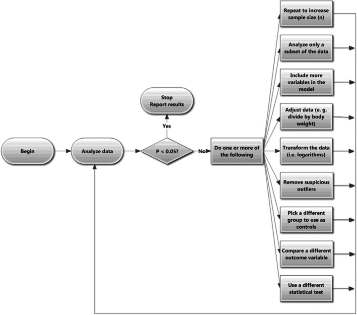
Statistical results can only be interpreted at face value when every choice in data analysis was performed exactly as planned and documented as part of the experimental design. From my conversations with scientists, it seems that this rule is commonly broken in reports of basic research. Instead, analyses are often done as shown in Figure 1. Collect and analyze some data. If the results are not statistically significant but show a difference or trend in the direction you expected, collect some more data and reanalyze. Or try a different way to analyze the data: remove a few outliers; transform to logarithms; try a nonparametric test; redefine the outcome by normalizing (say, dividing by each animal's weight); use a method to compare one variable while adjusting for differences in another; the list of possibilities is endless. Keep trying until you obtain a statistically significant result or until you run out of money, time, or curiosity.

Figure 1.

The many forms of P-hackingWhen you P-hack, the results cannot be interpreted at face value. Not shown in the figure is that after trying various forms of P-hacking without getting a small P values, you will eventually give up when you run out of time, funds or curiosity.

The results from data collected this way cannot be interpreted at face value. Even if there really is no difference (or no effect), the chance of finding a ‘statistically significant’ result exceeds 5%. The problem is that you introduce bias when you choose to collect more data (or analyze the data differently) only when the P value is greater than 0.05. If the P value was less than 0.05 in the first analyses, it might be larger than 0.05 after collecting more data or using an alternative analysis. But you'd never see this if you only collected more data or tried different data analysis strategies when the first P value was greater than 0.05.

Exploring your data can be a very useful way to generate hypotheses and make preliminary conclusions. But all such analyses need to be clearly labeled, and then retested with new data.

There are three related terms that describe this problem:

• Ad hoc sample size selection. This is when you didn't choose a sample size in advance, but just kept going until you liked the results. Figure 2 demonstrates the problem with ad hoc sample size determination. Distinguish unplanned ad hoc sample size decisions from planned ‘adaptive’ sample size methods that make you ‘pay’ for the increased versatility in sample size collection by requiring a stronger effect to reach ‘significance’ (FDA 2010; Kairalla et al., 2012).

• Hypothesizing After the Result is Known (HARKing, Kerr 1998). This is when you analyze the data many different ways (say different subgroups), discover an intriguing relationship, and then publish the data so it appears that the hypothesis was stated before the data were collected (Figure 3). This is a form of multiple comparisons (Berry, 2007). Kriegeskorte and colleagues (2009) call this double dipping, as you are using the same data both to generate a hypothesis and to test it.

• P-hacking. This is a general term that encompasses dynamic sample size collection, HARKing, and more. It was coined by Simmons et al. (2011) who also use the phrase, ‘too many investigator degrees of freedom’. P-hacking is especially misleading when it involves changing the actual values analyzed. Examples include ad hoc sample size selection (see above), switching to an alternate control group (if you don't like the first results and your experiment involved two or more control groups), trying various combinations of independent variables to include in a multiple regression (whether the selection is manual or automatic), and analyzing various subgroups of the data. Reanalyzing a single data set in various ways is also P-hacking but won't usually mislead you quite as much.

Figure 2.

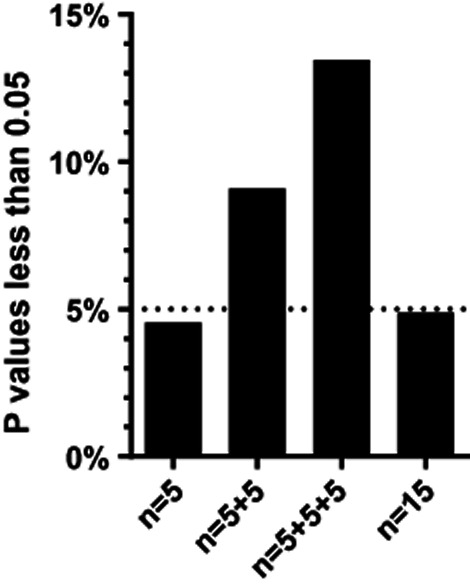
The problem of ad hoc sample size selectionI simulated 10,000 experiments sampling data from a Gaussian distribution with means of 5.0 and standard deviations of 1.0, and comparing two samples with n = 5 each using an unpaired t test. The first column shows the percentage of those experiments with a P value less than 0.05. Since both populations have the same mean, the null hypothesis is true and so (as expected) about 5.0% of the simulations have P values less than 0.05. For the experiments where the P value was higher than 0.05, I added five more values to each group. The middle column (‘n = 5 + 5’) shows the fraction of P values where the P value was less than 0.05 either in the first analysis with n = 5 or after increasing the sample size to 10. For the third column, I added yet another 5 values to each group if the P value was greater than 0.05 for both of the first two analyses. Now 13% of the experiments (not 5%) have reached a P value less than 0.05. For the fourth column, I looked at all 10,000 of the simulated experiments with n = 15. As expected, very close to 5% of those experiments had P values less than 0.05. The higher fraction of ‘significant’ findings in the n = 5 + 5 and n = 5 + 5 + 5 is due to the fact that I increased sample size only when the P value was high with smaller sample sizes. In many cases, when the P value was less than 0.05 with n = 5 the P value would have been higher than 0.05 with n = 10 or 15, but an experimenter seeing the small P value with the small sample size would not have increased sample size.

Figure 3.

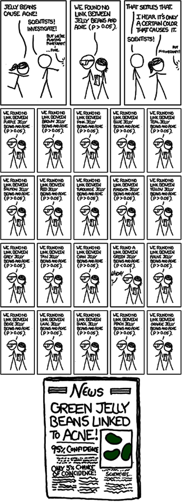
The problem of Hypothesizing After the Results are Known (HARKing)From http://xkcd.com/882/.

My suggestion for authors:

• For each figure or table, clearly state whether or not the sample size was chosen in advance, and whether every step used to process and analyze the data was planned as part of the experimental protocol.

• If you use any form of P-hacking, label the conclusions as ‘preliminary.’

Misconception 2: P values convey information about effect size

To compute a P value, you first must clearly define a null hypothesis, usually that two means (or proportions or EC50s…) are identical. Given some assumptions, the P values is the probability of seeing an effect as large as or larger than you observed in the current experiment if in fact the null hypothesis was true. But note that the P value gives you no information about how large the difference (or effect) is. Figure 4 demonstrates this point by plotting the P values that result from comparing two samples in experiments with different sample sizes. Even though the means and standard deviations are identical for each simulated experiment, the P values are far from identical. With n = 3 in each group, the P value is 0.65. When n = 300 in each group, the P value is 0.000001.

Figure 4.

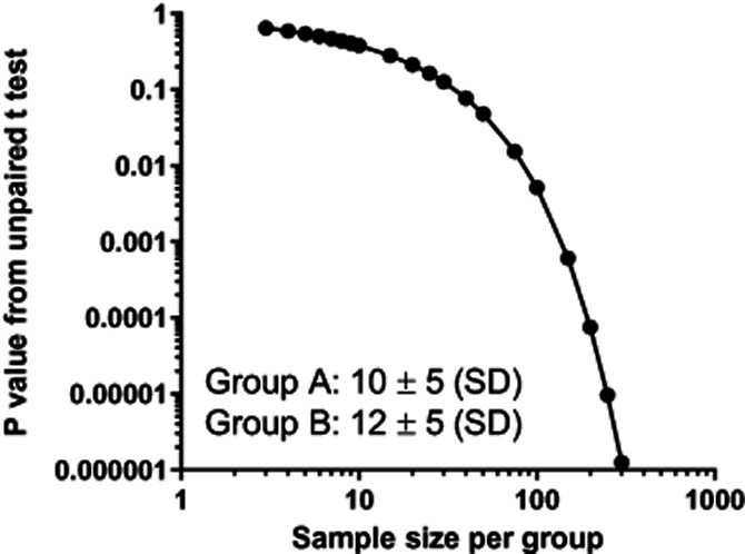
P values depend upon sample sizeThis graph shows P values computed by unpaired t tests comparing two sets of data. The means of the two samples are 10 and 12. The S.D. of each sample is 5.0. I computed a t test using various sample sizes plotted on the X axis. You can see that the P value depends on sample size. Note that both axes use a logarithmic scale.

The dependence of P values on sample size can lead to two problems.

A large P value is not proof of no (or little) effect

The top two rows of Table 1 presents the results of two simulated experiments. The two P values are both about 0.6, but the two experiments lead to very different conclusions.

Table 1.

Identical P values with very different interpretations

	Treatment 1 (mean ± SD, n)	Treatment 2 (mean ± SD, n)	Difference between means	P value	95% CI of the difference between means
Experiment A	1000 ± 100, n = 50	990.0 ± 100, n = 50	10	0.6	−30 to 50
Experiment B	1000 ± 100, n = 3	950.0 ± 100, n = 3	50	0.6	−177 to 277
Experiment C	100 ± 5.0, n = 135	102 ± 5.0, n = 135	2	0.001	0.8 to 3.2
Experiment D	100 ± 5.0, n = 3	135 ± 5.0, n = 3	35	0.001	24 to 46

Experiments A and B have identical P values, but the scientific conclusion is very different. The interpretation depends upon the scientific context, but in most fields Experiment A would be solid negative data proving that there either is no effect or that the effect is tiny. In contrast, Experiment B has such a wide confidence interval as to be consistent with nearly any hypothesis. Those data simply do not help answer your scientific question.

Similarly, experiments C and D have identical P values, but should be interpreted differently. In most experimental contexts, experiment C demonstrates convincingly that while the difference not zero, it is quite small. Experiment D provides convincing evidence that the effect is large.

In experiment A (from Table 1) the difference between means in the experimental sample is 10, so the difference equals 1% of the mean of treatment 1. Assuming random sampling from Gaussian populations, the 95% confidence interval for the difference between the two population means ranges from −30 to 50. In other words the data are consistent (with 95% confidence) with a decrease of 3%, an increase of 5%, or anything in between. The interpretation depends on the scientific context and the goals of the experiment, but in most contexts these results can be summarized simply: The data are consistent with a tiny decrease, no change, or a tiny increase. These are solid negative data.

Experiment B is very different. The difference between means is larger, and the confidence interval is much wider (because the sample size is so small). Assuming random sampling from Gaussian populations, the data are consistent (with 95% confidence) with anything between a decrease of 18% and an increase of 28%. The data are consistent with a large decrease, a small decrease, no difference, a small increase, or a large increase. These data lead to no useful conclusion at all! An experiment like this should not be published.

A small P value is not proof of a large effect

The bottom two rows of Table 1 presents the results of two simulated experiments where both P values are 0.001, but again two experiments lead to very different conclusions.

In experiment C (from Table 1) the difference between means in the experimental sample is only 2 (so the difference equals 2% of the mean of treatment 1). Assuming random sampling from Gaussian populations, the 95% confidence interval for the difference between the two population means ranges from 0.8 to 3.2. In other words the data are consistent (with 95% confidence) with anything between an increase of 0.8% and an increase of 3.2%. How to interpret that depends on the scientific context and the goals of the experiment, but in most contexts this can be summarized simply: The data clearly demonstrate an increase, but that increase is tiny.

Experiment D is very different. The difference between means is 35 (so 35% of the control mean), and the confidence interval extends from an increase of 23.7% to an increase of 46.3%. The data clearly demonstrate that there is an increase that is (with 95% confidence) substantial.

My suggestions for authors:

• Always show and emphasize the effect size (as difference, percent difference, ratio, or correlation coefficient) along with its confidence interval.

• Consider omitting reporting of P values.

Misconception 3: Statistical hypothesis testing and reports of ‘statistical significance’ are necessary in experimental research

Statistical hypothesis testing is a way to make a crisp decision from one analysis. If the P value is less than a preset value (usually 0.05), the result is deemed ‘statistically significant’ and you make one decision. Otherwise the result is deemed ‘not statistically significant’ and you make the other decision. This is helpful in quality control and some clinical studies. It also is useful when you rigorously compare the fits of two scientifically sensible models to your data, and choose one to guide your interpretation of the data and to plan future experiments.

Here are five reasons to avoid use of statistical hypothesis testing in experimental research:

• The need to make a crisp decision based on one analysis is rare in basic research. A decisions about whether or not to place an asterisk on a figure doesn't count! If you are not planning to make a crisp decision, the whole idea of statistical hypothesis testing is not helpful.

• Statistical hypothesis testing ‘does not tell us what we want to know, and we so much want to know what we want to know that, out of desperation, we nevertheless believe that it does!’ (Cohen, 1994). Statistical hypothesis testing has even been called a cult (Ziliak and McCloskey, 2008). The question we want to answer is: Given these data, how likely is the null hypothesis? The question that a P values answers is: Assuming the null hypothesis is true, how unlikely are these data? These two questions are distinct, and so have distinct answers.

• Scientists who intend to use statistical hypothesis testing often end up not using it. If the P value is just a bit larger than 0.05, scientists often avoid the strict use of hypothesis testing and instead apply the ‘time-honoured tactic of circumlocution to disguise the non-significant result as something more interesting’ (Hankins, 2013). They do this by using terms such as ‘almost significant’, ‘bordered on being statistically significant’, ‘a statistical trend toward significance’, or ‘approaching significance’. Hankins lists 468 such phrases he found in published papers!

• The 5% significance threshold is often misunderstood. If you use a P value to make a decision, of course it is possible that you will make the wrong decision. In some cases, the P value will be tiny just by chance, even though the null hypothesis of no difference is actually true. In these cases a conclusion that a finding is statistically significant is a false positive and you will have made what is called a Type I error2010. Many scientists mistakenly believe that the chance of making a false positive conclusion is 5%. In fact, in many situations the chance of making a Type I false positive conclusion is much higher than 5% (Colquhoun 2014). For example, in a situation where you expect the null hypothesis to be true 90% of the time (say you are screening lightly prescreened compounds, so expect 10% to work), you've chosen a sample size large enough to ensure 80% power, and you use the traditional 5% significance level, the false discovery rate is not 5% but rather is 36% (the calculations are shown in Table 2). If you only look at experiments where the P value is just a tiny bit less than 0.050, the probability of a false positive rises to 79% (Motulsky, 2014b). Ioannidis (2005) used calculations like these (and other considerations) to argue that most published research findings are probably false.

• The word ‘significant’ is often misunderstood. The problem is that ‘significant’ has two distinct meanings in science (Motulsky, 2014c). One meaning is that a P value is less than a preset threshold (usually 0.05). The other meaning of ‘significant’ is that an effect is large enough to have a substantial physiological or clinical impact. These two meanings are completely different, but are often confused.

Table 2.

The false discovery rate when P < 0.05

	P < 0.05	P > 0.05	Total
Really is an effect	80	20	100
No effect (null hypothesis true)	45	855	900
Total	125	875	1000

This table tabulates the theoretical results of 1000 experiments where the prior probability that the null hypothesis is false is 10%, the sample size is large enough so that the power is 80%, and the significance level is the traditional 5%. In 100 of the experiments (10%) there really is an effect (the null hypothesis is false), and you'll obtain a ‘statistically significant’ result (P < 0.05) in 80 of these (because the power is 80%). In 900 experiments, the null hypothesis is true but you'll obtain a statistically significant result in 45 of them (because the significance threshold is 5% and 5% of 900 is 45). In total you will obtain 80 + 45 = 125 statistically significant results, but 45/125 = 36% of these will be false positive. The proportion of conclusions of ‘statistical significance’ that are false discoveries or false positives depends on the context of the experiment, as expressed by the prior probability (here 10%).

If you do obtain a small P value and reject the null hypothesis, you'll conclude that the values in the two groups were sampled from different distributions. As noted above, there may be a high chance that you made a false positive conclusion due to random sampling. But even if the conclusion is ‘true’ from a statistical point of view and not a false positive due to random sampling, the effect may have occurred for a reason different than the one you hypothesized. When thinking about why an effect occurred, ignore the statistical calculations, and instead think about blinding, randomization, positive controls, negative controls, calibration, biases, and other aspects of experimental design.

My suggestions for authors:

• Only report statistical hypothesis testing (and place significance asterisks on figures) when you will make a decision based on that one analysis.

• Never use the word ‘significant’ in a scientific paper. If you use statistical hypothesis testing to make a decision, state the P value, your preset P value threshold, and your decision. When discussing the possible physiological or clinical impacts of a finding, use other words.

Misconception 4. The standard error of the mean quantifies variability

Pharmacology journals are full of graphs and tables showing the mean and the standard error of the mean (S. E. M.).

A quick review. The standard deviation (S.D.) quantifies variation among a set of values, but the SEM does not. The S.E.M. is computed by dividing the S.D. by the square root of sample size. With large samples, the S.E.M. will be tiny even if there is a lot of variability.

One problem with plotting or displaying the mean ± S.E.M. is that some people viewing the graph or table may mistakenly think that the error bars show the variability of the data. A second problem with reporting means with S.E.M. is that the range mean ± S.E.M. cannot be rigorously interpreted. The S.E.M. gives information about how precisely you have determined the population mean. So the range mean ± S.E.M. is a confidence interval, but the confidence level depends on sample size. With large samples, that range is a 68% confidence interval of the mean. When n = 3, that range is only a 58% confidence interval2013.

My suggestions for authors:

• If you want to display the variability among the values, show raw data (which is not done often enough in my opinion). If showing the raw data would make the graph hard to read, show instead a box-whisker plot, a frequency distribution, or the mean and SD.

• If you want readers to see how precisely you have determined the mean, report a confidence interval (95% confidence intervals are standard). Figure 5 shows a dataset plotted using all of these methods.

• When reporting results from regression, show the 95% confidence interval of each parameter rather than standard errors.

Figure 5.

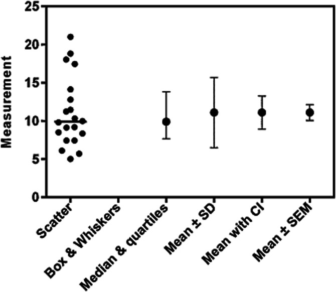
Standard error bars do not show variability and do a poor job of showing precision.The figure plots one data set six ways. The leftmost lane shows a scatter plot of every value, so is the most informative. The next lane shows a box-and-whisker plots showing the range of the data, the quartiles, and the median (whiskers can be plotted in various ways, and don't always show the range). The third lane plots the median and quartiles. This shows less detail, but still demonstrates that the distribution is a bit asymmetrical. The fourth lane plots mean with error bars showing plus or minus one standard deviation. Note that these error bars are, by definition, symmetrical so give you no hint about the asymmetry of the data. The next two lanes are different than the others as they do not show scatter. Instead they show how precisely we know the population mean, accounting for scatter and sample size. The fifth lane shows the mean with error bars showing the 95% confidence interval of the mean. The sixth (rightmost) lane plots the mean plus or minus one standard error of the mean, which does not show variation and does a poor job of showing precision.

Misconception 5: You don't need to report the details

The methods section of every paper should report the methods with enough detail that someone else could reproduce your work. This applies to statistical methods just as it does to experimental methods.

My suggestions for authors:

• When reporting a sample size, explain exactly what you counted. Did you count replicates in one experiment (technical replicates), repeat experiments, the number of studies pooled in a meta-analysis, or something else?

• If you eliminated any outliers, state how many outliers you eliminated, the rule used to identify them, and a statement whether this rule was chosen before collecting data.

• If you normalized data, explain exactly how you defined 100% and 0%.

• When possible, report the P value up to at least a few digits of precision, rather than just stating whether the P value is less than or greater than an arbitrary threshold. For each P value, state the null hypothesis it tests if there is any possible ambiguity.

• When reporting a P value that compares two groups, state whether the P value is one- or two-tailed. If you report a one-tailed P value, state that you recorded a prediction for the direction of the effect (for example increase or decrease) before you collected any data and what this prediction was. If you didn't record such a prediction, report a two-tailed P value.

• Explain the details of the statistical methods you used. For example, if you fit a curve using nonlinear regression, explain precisely which model you fit to the data and whether (and how) data were weighted. Also state the full version number and platform of the software you use.

• Consider posting files containing both the raw data and the analyses so other investigators can see the details.

Summary

The physicist E. Rutherford supposedly said, ‘If your experiment needs statistics, you ought to have done a better experiment2005.’ There is a lot of truth to that statement when you are working in a field with a very high signal to noise ratio. In these fields, statistical analysis may not be necessary. But if you work in a field with a lower signal/noise ratio, or are trying to compare the fits of alternative models that don't differ all that much, you need statistical analyses to properly quantify your confidence in your conclusions.

I suspect that one of the reasons that the results reported in many papers cannot be reproduced is that statistical analyses are often done as a quick afterthought, with the goal to sprinkle asterisks on figures and the word ‘significant’ on conclusions. The suggestions I propose in this editorial can all be summarized simply: If you are going to analyze your data using statistical methods, then plan the methods carefully, do the analyses seriously, and report the data, methods and results completely.

Conflict of interest

The author is employed by GraphPad Software Inc. Publication of this article in BJP does not indicate an endorsement of GraphPad Software.

References

- Anonymous. Trouble at the lab. The Economist. 2013;409:23–27. 2013. [Google Scholar]
- Collins FS, Tabak LA. Policy: NIH plans to enhance reproducibility. Nature. 2014;505:612–613. doi: 10.1038/505612a. [DOI] [PMC free article] [PubMed] [Google Scholar]
- Begley CG, Ellis LM. Raise standards for preclinical cancer research. Nature. 2012;483:533. doi: 10.1038/483531a. [DOI] [PubMed] [Google Scholar]
- Berry DA. The difficult and ubiquitous problems of multiplicities. Pharmaceutical Stat. 2007;6:155–160. doi: 10.1002/pst.303. [DOI] [PubMed] [Google Scholar]
- Cohen J. The earth is round (p < 0.05) Amer. Psychologist. 1994;49:997–1003. [Google Scholar]
- Colquhoun D. 2014. An investigation of the false discovery rate and the misinterpretation of P values http://arxiv.org/abs/1407.5296.
- FDA. 2010. Guidance for Industry: Adaptive Design Clinical Trials for Drugs and Biologics. Accessed July 29, 2014 at http://www.fda.gov/downloads/Drugs/GuidanceComplianceRegulatoryInformation/Guidances/UCM201790.pdf.
- Hankins M. 2013. Still not significant. Psychologically Flawed April 21. Accessed July 28, 2013 at mchankins.wordpress.com/2013/04/21/still-not-significant-2/
- Ioannidis JPA. Why most published research findings are false. PLoS Med. 2005;2:e124. doi: 10.1371/journal.pmed.0020124. [DOI] [PMC free article] [PubMed] [Google Scholar]
- Kairalla JA, Coffey CS, Thomann MA, Muller KE. Adaptive trial designs: a review of barriers and opportunities. Trials. 2012;13:145–145. doi: 10.1186/1745-6215-13-145. [DOI] [PMC free article] [PubMed] [Google Scholar]
- Kerr NL. HARKing: Hypothesizing after the results are known. Personality and Social Psychology Review. 1998;2:196–217. doi: 10.1207/s15327957pspr0203_4. [DOI] [PubMed] [Google Scholar]
- Kriegeskorte N, Simmons WK, Bellgowan PSF, Baker CI. Circular analysis in systems neuroscience: The dangers of double dipping. Nature Neuroscience. 2009;12:535–540. doi: 10.1038/nn.2303. [DOI] [PMC free article] [PubMed] [Google Scholar]
- Marino MJ. The use and misuse of statistical methodologies in pharmacology research. Biochem Pharmacol. 2014;87:78–92. doi: 10.1016/j.bcp.2013.05.017. [DOI] [PubMed] [Google Scholar]
- Motulsky HJ. Intuitive Biostatistics. 3. Oxford University Press; 2014a. edition. [Google Scholar]
- Motulsky HJ. 2014b. Using simulations to calculate the false discovery rate. Accessed June 1, 2014 at http://www.graphpad.com/support/faqid/1923.
- Motulsky HJ. Opinion: Never use the word ‘significant’ in a scientific paper. Adv Regenerative Biology. 2014c;1:25155. 2014, http://dx.doi.org/10.3402/arb.v1.25155 (in press) [Google Scholar]
- Prinz F, Schlange T, Asadullah K. Believe it or not: how much can we rely on published data on potential drug targets? Nat Rev Drug Discovery. 2011;10:712–713. doi: 10.1038/nrd3439-c1. . DOI 10.1038/ [DOI] [PubMed] [Google Scholar]
- Simmons J, Nelson L, Simonsohn U. False-positive psychology: Undisclosed flexibility in data collection and analysis allow presenting anything as significant. Psychological Science. 2011;22:1359–1366. doi: 10.1177/0956797611417632. [DOI] [PubMed] [Google Scholar]
- Ziliak S, McCloskey DN. The cult of statistical significance: How the standard error costs us jobs, justice, and lives. Ann Arbor: University of Michigan Press; 2008. . ISBN= 0472050079. [Google Scholar]