3D structure tensor analysis of light microscopy data for validating diffusion MRI

Abstract

Diffusion magnetic resonance imaging (d-MRI) is a powerful non-invasive and non-destructive technique for characterizing brain tissue on the microscopic scale. However, the lack of validation of d-MRI by independent experimental means poses an obstacle to accurate interpretation of data acquired using this method. Recently, structure tensor analysis has been applied to light microscopy images, and this technique holds promise to be a powerful validation strategy for d-MRI. Advantages of this approach include its similarity to d-MRI in terms of averaging the effects of a large number of cellular structures, and its simplicity, which enables it to be implemented in a high-throughput manner. However, a drawback of previous implementations of this technique arises from it being restricted to 2D. As a result, structure tensor analyses have been limited to tissue sectioned in a direction orthogonal to the direction of interest. Here we describe the analytical framework for extending structure tensor analysis to 3D, and utilize the results to analyze serial image “stacks” acquired with confocal microscopy of rhesus macaque hippocampal tissue. Implementation of 3D structure tensor procedures requires removal of sources of anisotropy introduced in tissue preparation and confocal imaging. This is accomplished with image processing steps to mitigate the effects of anisotropic tissue shrinkage, and the effects of anisotropy in the point spread function (PSF). In order to address the latter confound, we describe procedures for measuring the dependence of PSF anisotropy on distance from the microscope objective within tissue. Prior to microscopy, ex vivo d-MRI measurements performed on the hippocampal tissue revealed three regions of tissue with mutually orthogonal directions of least restricted diffusion that correspond to CA1, alveus and inferior longitudinal fasciculus. We demonstrate the ability of 3D structure tensor analysis to identify structure tensor orientations that are parallel to d-MRI derived diffusion tensors in each of these three regions. It is concluded that the 3D generalization of structure tensor analysis will further improve the utility of structure tensor analyses for d-MRI by making it a more flexible experimental technique that closer resembles the inherently 3D nature of d-MRI measurements.

INTRODUCTION

In studies of brain development, aging, and pathology, it is often desirable to quantify cellular morphological changes, or differences in cell morphology between a perturbed and a control condition. Unfortunately, traditional anatomical methods for quantifying such differences involve time consuming, operator-dependent procedures (Parekh and Ascoli, 2013). This problem is compounded in quantitative studies by the need to characterize large numbers of cells to detect potentially subtle morphological effects. Diffusion magnetic resonance imaging (d-MRI) techniques have the favorable property that large ensembles of cells present within an MRI voxel contribute to each measurement. In addition, d-MRI is commonly capable of characterizing cells in 3D throughout the brain in a non-invasive manner (Basser and Pierpaoli, 1996; Le Bihan, 2003; Mori et al., 2005). For these reasons, d-MRI is frequently utilized to study cellular-level anatomy in brain white matter (Beaulieu, 2011; Jones et al., 2013), as well as in gray matter (Bozzali et al., 2002; D’Arceuil and Crespigny, 2010; Jespersen et al., 2007; Zhang et al., 2002). A primary difficulty encountered with d-MRI, however, is the inability to interpret quantitative indices of water diffusion in terms of underlying cellular structure. Mathematical modeling of water diffusion combined with independent experimental validation (Gao et al., 2013; Jespersen et al., 2010; Jespersen et al., 2012; Leergaard et al., 2010b; Wang et al., 2011; Wedeen et al., 2008), are instrumental for developing the ability to interpret d-MRI measurements in terms of specific properties of underlying biological tissue. However, as a result of the difficulties of traditional methods, independent experimental validation is only available for a small subset of the experimental contexts in which d-MRI has been applied.

In a notable recent advance, Budde and co-workers applied structure tensor analysis of images obtained by light microscopy as a strategy to validate d-MRI findings (Budde and Frank, 2012). In their implementation, computation of the structure tensor for a given image pixel first involves determining direction-dependent spatial derivatives of image intensity near the pixel, and second, averaging the products of spatial derivatives over a user-specified neighborhood of the pixel. As described in detail in the following sections, this procedure shares several similarities to d-MRI measurements. Briefly, the length-scale used for calculating spatial derivatives is somewhat comparable to the displacement distance experienced by a water molecule, which is determined by the diffusion time of a d-MRI measurement. Second, the neighborhood size specified for averaging spatial derivatives is analogous to the image resolution, or voxel size of a d-MRI experiment. As a result, structure tensor calculations provide information related to ensembles of many cellular features, as is true for d-MRI. Advantages of structure tensor analyses compared to other validation strategies are its ease of automated implementation, such that it can be applied to several experimental subjects in experiments designed to compare multiple groups; it can be used to analyze microscopy data obtained using virtually any staining method (Budde and Annese, 2013); and the directional information provided by the structure tensor can be compared to that of the diffusion tensor (Budde et al., 2011). One drawback to previous structure tensor implementations, however, is that they have been limited to two dimensions, whereas for d-MRI analyses, 3D measurements are standard. As a consequence, 2D structure tensor analyses must be performed on tissue that is sectioned in a frame that is parallel to the local cellular primary axis to be characterized. For cases in which the local axis system orientation is unknown, or if more than one principal axis system is present within a sample, 2D structure tensor analyses are of limited value for validating d-MRI.

Here we present methods to extend previous structure tensor analyses to 3D. The analytical expressions used in the 2D implementation (Budde and Frank, 2012) are straightforwardly generalized to 3D. In order to demonstrate the technique, a 3D “stack” of confocal microscope images are acquired of gray matter and associated white matter of hippocampal tissue obtained from an adult rhesus macaque brain that had previously undergone ex vivo d-MRI, and was subsequently sectioned and stained with DiI following the procedures of Budde et al. (Budde and Frank, 2012). The region of tissue analyzed by the 3D structure tensor method was shown by d-MRI to contain three regions, with each region exhibiting a microscopic principal orientation parallel to the x, y, and z axes of the laboratory frame. For accurate 3D structure tensor analyses, multiple image transformations are necessary to remove experimentally-introduced sources of anisotropy associated with tissue preparation and measurement using a confocal microscope. Following these steps, it is demonstrated that 3D structure tensor orientations parallel to the principal directions measured by d-MRI are obtained within the hippocampal tissue section.

MATERIALS AND METHODS

Hippocampal brain tissue was obtained from a 13-year-old (middle-aged adult) female rhesus macaque. Following cerebral perfusion fixation with 4% paraformaldehyde, the brain was immersed in 4% paraformaldehyde for 24 hours and subsequently transferred to phosphate-buffered saline (PBS). The brain was sectioned into 5 mm-thick coronal blocks as described in (Daunais et al., 2010), and the left hippocampus and associated white matter, including the alveus and inferior longitudinal fasciculus (ILF), was extracted for ex-vivo MRI and histological analyses (Fig. 1). All experimental protocols and animal handling procedures were according to the guideline stipulated by NIH “Guide for the Care and Use of Laboratory Animals” (NIH, 1987) and were approved by the OHSU animal care and use committee.

Figure 1.

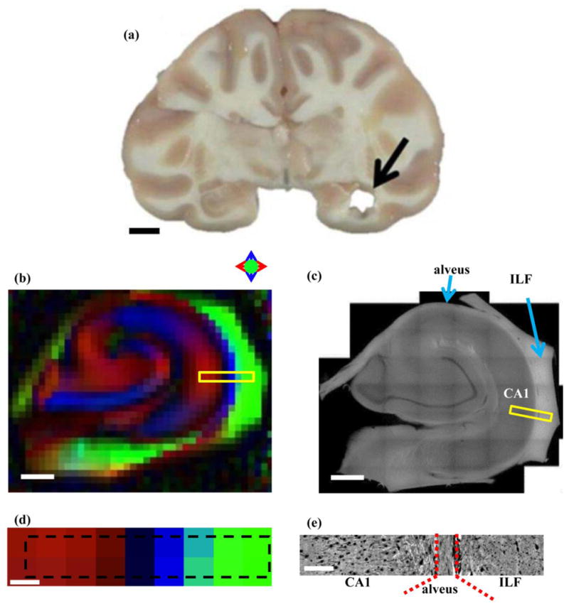
(a) Coronal section of rhesus macaque brain following dissection of hippocampal tissue analyzed in this study. (b) Directional diffusion FA map of hippocampus. Anisotropic diffusion oriented in the left/right, up/down, and in/out of plane directions are indicated by red, blue, and green colors, as described in the text. (c) A 2D montage of a 200 μm-thick hippocampal tissue section obtained at 10x magnification using 3D confocal microscopy. (d) Directional FA map of the region subsequently analyzed by 3D confocal microscopy. Dashed black rectangle indicates the location of the yellow box in Fig. 1b, and corresponds to the location indicated by the yellow box in Fig. 1c. (e) One slice of the 3D image acquired at 63x magnification, digitized at 0.25μm resolution on confocal microscope. Scale bars (a) 10 mm, (b) and (c) 1mm, (d) and (e) 200 μm; Abbreviations: ILF: Inferior longitudinal fasciculus; CA: Cornu Ammonis.

Diffusion Magnetic Resonance Imaging (d-MRI)

Ex vivo d-MRI was performed on an 11.7 T small-animal MRI system with a 30 cm clear bore magnet (Bruker, Rheinstetten, Germany) interfaced with 9 cm inner diameter magnetic field gradient coil. The tissue was immersed in PBS and held in a sample tube that fit within a 20 mm-diameter solenoid transmit/receive radiofrequency (Dauguet et al., 2007) coil. A multi-slice spin-echo pulse sequence incorporating a StejskalqTanner diffusion sensitization gradient pair was used to acquire d-MRI data. The diffusion weighting factor (b-value) was 2500 s/mm² with a gradient duration and separation of δ = 12ms and Δ = 21 ms, respectively, a gradient strength g = 11.6 G/cm, an echo time TE = 42 ms, and a recycle delay TR = 12.5 s. The image resolution was isotropic with 200 μm-sided voxels. Ten scans were acquired in which b = 0, and diffusion anisotropy was measured using a 63-direction diffusion sampling scheme, which consisted of 60 directions determined by an electrostatic repulsion algorithm (Jones et al., 1999), plus the three laboratory-frame vectors (1,0,0), (0,1,0), and (0,0,1). The length of the diffusion acquisition was 4 hours and 23 minutes. Diffusion tensor imaging metrics such as fractional anisotropy (FA) were calculated from the diffusion-weighted images using standard procedures (Basser and Pierpaoli, 1996; Batchelor et al., 2003). An FA map that is color-coded to indicate the direction of least restricted diffusion from a central slice within the tissue block is shown in Fig. 1d. In Fig. 1d and subsequent figures, the red, green, and blue (rgb) channels of directional FA maps are scaled by the x, y, and z components, respectively, of the primary eigenvector (v₁) and FA. The rgb vector for each pixel is ( ${\mathit{FAv}}_{1,x}^2,{\mathit{FAv}}_{1,y}^2,{\mathit{FAv}}_{1,z}^2$).

Histological procedures

Subsequent to d-MRI, the 5 mm thick sections of dissected hippocampal tissue were further sub-sectioned at 200 μm with a vibratome as described in (Leigland et al., 2013), and staining procedures described in (Budde and Frank, 2012) were followed. In brief, sections were dehydrated with graded concentrations of ethanol and stained with a fluorescent lipophilic dye (1, 1′-Dioctadecyl-3,3,3′,3′-tetra-methylindocarbocyanine, or “DiI”) in absolute alcohol (0.25 mg/ml) for approximately 3 minutes. The stained sections were then rinsed with absolute ethanol to remove excess dye and then rehydrated by reversing the order of graded ethanol concentrations used for dehydration. Sections were mounted on glass slides with Prolong Antifade Gold mounting medium (Invitrogen, Molecular Probes).

Microscopy

A 2D montage of an entire tissue section obtained from the center of the 5 mm block was constructed at 10x magnification using a (Leica Microsystems, Bannockburn, IL) (Fig. 1c). For one subsection (yellow rectangle, Fig. 1c), chosen based on the presence of three regions in which the primary diffusion tensor eigenvector is parallel to the x, y, and z directions of the imaging frame, a 3D montage was obtained using a Leica SP5 AOBS microscope (Leica Microsystems, Bannockburn, IL) equipped with a Leica objective (HCX PLAPO CS63x 1.40 Oil). The images were acquired with isotropic digital resolution of 0.25 μm-sided voxels. After converting images to tif format, they were imported into Matlab (The Mathworks, Natick, MA) for subsequent steps of image analysis. Slices from the 3D montage are shown in Fig. 1e. Several orthogonal slices of the 3D images of the image stack are shown in figure 2.

Figure 2.

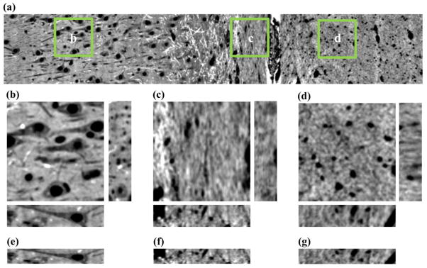
(a) An xy slice of the 3D montage acquired using a 63x objective. Regions (b–d) show magnified xy, xz (lower), and yz (right) planes from the labeled green squares in (a). The xz planes prior shrinkage correction are shown in (e–g).

Structure Tensor Analysis

The published formulas for computing 2D structure tensors (Budde and Frank, 2012) are straightforwardly generalized to 3D. At each point (x, y, z) in a 3D image I(x, y, z), the spatial derivative with respect to x is abbreviated

$$I_x(x,y,z)=\frac{\partial }{\partial x}I(x,y,z)$$ [1]

and similarly for y and z. As a practical matter, the common method for computing spatial derivatives involves first convolving the image with a Gaussian kernel. For the procedures implemented in this study, the spatial derivatives were thus calculated according to the formula

$$I_x(x,y,z)=-(1/{\sigma }^2)[x^{\prime }G(x^{\prime },y^{\prime },z^{\prime })\ast I(x^{\prime },y^{\prime },z^{\prime })](x,y,z)$$ [2]

and similarly for y and z, and where the convolution operation is represented by “[*]” and G is the Gaussian kernel

$$G(x,y,z)=\frac{1}{\sqrt{2\pi {\sigma }^2}}exp\left(-\left[x^2+y^2+z^2\right]/(2{\sigma }^2)\right).$$ [3]

Thus, the size of the local region used for computing spatial derivatives is determined by the value chosen for the kernel width σ. Varying σ in structure tensor calculations is somewhat analogous to varying the diffusion time (and hence the root mean squared molecular displacement) in d-MRI experiments, because both parameters in principle influence the size of the local environment that contributes to the structure tensor, or diffusion tensor, at a given point. Specifically, the convolution operation implements a local average over a region of characteristic size σ, whereas the diffusion process itself averages local structural fluctuations on the scale of the diffusion length – and can in fact be shown to correspond to the convolution with a Gaussian filter of width equal to the diffusion length (Novikov et al., 2014). Nevertheless, it should of course be kept in mind that structural features that influence staining and water diffusion may be different. At each voxel location, the above operations enable the image gradient vector ∇I = (I_x, I_y, I_z) to be constructed, the direction of which is the direction of the fastest intensity variation. This direction is expected to be perpendicular to any boundary passing through the pixels used to compute the derivatives.

As an example, a synthetic image was constructed in which voxels inside a cylinder (Fig. 3a) differ in intensity from voxels outside of a cylinder. Gradients for this image are illustrated in Fig. 3b.

Figure 3.

(a) A synthetic image of a solid cylinder was constructed for illustrating properties of the structure tensor. Here only the surface of the cylinder is shown. (b) A subset of image intensity gradient vectors corresponding to (a) are shown. (c) Structure tensor eigenvectors (red, blue, and green) are shown together with the population of gradient vectors (black). The structure tensor eigenvector that corresponds to the minor eigenvalue (red) is parallel to the cylinder axis of symmetry. The two other eigenvectors correspond to eigenvalues equal in magnitude, and therefore assignment of the major eigenvector is arbitrary for this axially symmetric structure.

The structure tensor, S(x, y, z), is then computed by averaging products of the spatial derivatives over a specified neighborhood N

$$S(x,y,z)=\left(\begin{array}{ccc}{\langle I_x{I}_x\rangle }_N& {\langle I_x{I}_y\rangle }_N& {\langle I_x{I}_z\rangle }_N\\ {\langle I_y{I}_x\rangle }_N& {\langle I_y{I}_y\rangle }_N& {\langle I_y{I}_z\rangle }_N\\ {\langle I_z{I}_x\rangle }_N& {\langle I_z{I}_y\rangle }_N& {\langle I_z{I}_z\rangle }_N\end{array}\right).$$ [4]

in which 〈···〉_N denotes the average product over all points within N. As discussed in (Budde and Frank, 2012), there is flexibility in choosing a method of averaging, which may for example involve assigning weights to different points in the neighborhood. Choosing a size of N is analogous to setting the voxel size, or the image resolution, in a d-MRI experiment because both parameters influence the granularity with which the set of local probes of tissue structure are averaged. Equation (4) makes evident two factors that influence the size of structure tensor matrix elements. First, the magnitude of the gradient components I_x, I_y, and I_z will be reflected in the size of each of the products in the structure tensor matrix. Second, due to the averaging operation performed on each tensor element, gradient vectors with similar orientations will contribute more than terms derived from voxels with dis-similar gradient vector orientations. In this manner, Eq. 4 is similar to the scatter matrix of image gradient vectors over the neighborhood N. Equation 4 would be equal to the scatter matrix if the gradients were normalized by dividing by the length of the vector ∇I.

As described in 2D applications (Budde and Frank, 2012), the eigenvalues and eigenvectors of S are useful for characterizing structure tensor anisotropy. Here it is important to recognize a distinction between structure tensor and diffusion tensor analyses. In DTI, it is the eigenvector corresponding to the largest eigenvalue that is parallel to the primary structure orientation (such as a fiber bundle). However, in 2D structure tensor analyses, it is the direction of minimal image intensity variation, and hence the direction indicated by the eigenvector corresponding to the smallest eigenvalue, that is parallel to the primary structure orientation. This perspective also reveals an apparent difference between 2D and 3D structure tensor analysis. For example, if the averaging neighborhood is small compared to the radius of curvature of the boundary to be detected, the boundary appears locally planar and all gradient vectors point in nearly the same direction. Whereas this uniquely specifies the direction of a fiber bundle in two dimensions, i.e. the perpendicular direction, it does not do so in three dimensions. However, as long as the neighborhood is sufficiently large to include surface normals in more than one direction, the proper direction of the fiber bundle should be identified correctly by the third eigenvector of the 3D structure tensor. In practice, this is likely to be satisfied as soon as the averaging neighborhood can extend across the cross-section of the fiber bundle.

In the Fig. 3 example, the individual gradient vectors are translated to the origin of the Fig. 3c graph (black lines). The blue, green and red line segments indicate the orientations of the structure tensor major, middle, and minor eigenvectors (in this example, there is no difference between the major and middle eigenvalues, so these were arbitrarily assigned). Notably, it is the orientation of the minor eigenvector that is co-linear with the cylinder axis.

In a manner analogous to diffusion tensor imaging (DTI), fractional anisotropy of the structure tensor FA_ST is defined as

$${FA}_{ST}=\sqrt{\frac{1}{2}\frac{{({\tau }_1-{\tau }_2)}^2+{({\tau }_2-{\tau }_3)}^2+{({\tau }_3-{\tau }_1)}^2}{{\tau }_1^2+{\tau }_2^2+{\tau }_3^2}}$$ [5]

in which τ₁, τ₂, and τ₃ are the largest, middle, and smallest eigenvalues of S.

Prior to calculating structure tensors of the 3D image stack, it was necessary to perform three corrections to remove confounding sources of anisotropy that do not arise from properties of the DiI-stained tissue, but instead from properties of the measurement system/protocol. The first of these corrections was to de-trend the image intensity in the through-plane direction (parallel to the z-axis). In Fig. 4a, the average intensity in each x–y plane is plotted as a function of distance from the face of the glass coverslip separating the microscope objective from the tissue over the range spanning 0 micrometer (immediately adjacent to the coverslip) to 20 micrometers within the tissue. Example x–z planes are shown as insets of Fig. 4a and 4b. The approximately 2-fold reduction in intensity over this range results from a larger path length for light to the objective from deeper image planes, and consequent increased light scattering within the intervening tissue. If not corrected, this intensity variation would be a source of systematic bias in structure tensor anisotropy determinations. Therefore, to generate a z-profile corrected image, each x–y plane was divided by the mean image intensity within that plane. The resulting intensity plot and example x–z plane is shown in Fig. 4b.

Figure 4.

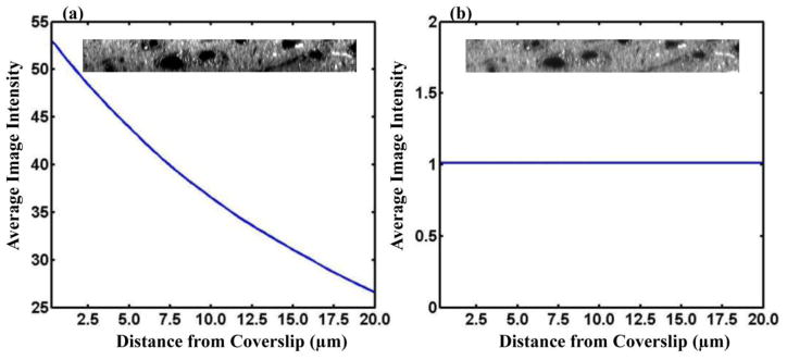
(a) Plot of average image intensity in the 3D montage as a function of distance from the coverslip. (b) Plot of average image intensity in 3D montage following intensity correction. Insets show yz slices before (a) and after (b) intensity bias correction.

The second correction performed on the image stack was to remove the effect of anisotropic tissue shrinkage. Through comparisons of distances between landmark structures in the MRI and light microscopy images, it was determined that the histological preparation procedures caused the tissue in the xy plane to shrink to 90% of the size it was when the d-MRI data was acquired. In contrast, shrinkage along the z-dimension was more severe. The average tissue thickness measured throughout the slice was 125 μm, as determined by adjusting the focal plane depth with the confocal microscope. For this sample, z-dimension shrinkage was remarkably homogeneous, with thickness varying by only 5% from the region with most extreme shrinkage in CA1 to the region with the smallest amount of z-dependent shrinkage in the ILF. The mean thickness of 125 μm is 62.5% of the thickness of the original section. To correct this source of anisotropy bias, the image was interpolated in the z direction by a factor of 1.44 (90/62.5) using the Matlab “interp” function to generate image voxels with isotropic dimensions relative to the original tissue. The x–z plane of Fig. 2b–d following this resampling is shown in Fig. 2e–g.

The final correction applied to the image was to compensate for the depth-dependent anisotropy of the confocal microscope’s point spread function (PSF). The PSF is the response of the microscope system to a point source of light. The measured image, M(x, y, z), is related to the underlying “true” image, U(x, y, z), through a convolution with the PSF: M = PSF*U.

The method of Cole and co-workers (Cole et al., 2011) was followed to measure the PSF by collecting 3D image stacks of 0.175±0.005 μm diameter red beads (Molecular Probes, Eugene), and approximating the PSF with an anisotropic 3D Gaussian function with standard deviations σ_x, σ_y, and σ_z, perpendicular to the x, y, and z axes, respectively. Due to the expectation that the microscope performance would degrade as a function of distance from the objective, a sample consisting of three layers of 40 μm-thick cerebral cortical brain tissue was constructed. Fluorescent beads were placed between the tissue and the cover slip, and between each layer of tissue. An image in the x–z plane from the serial stack used to measure the depth-dependent PSF is shown in Fig. 5a. Three layers of fluorescent beads are apparent. Within each layer, the Fiji plugin Metroloj (Matthews and Cordelières, 2010) was used to measure PSF σ_x, σ_y, and σ_z values from five beads. The mean values obtained from the 5 measurements at depths of 0 (the upper-most layer), 40 (the middle layer), and 80 μm (the lowest layer) are plotted in Fig. 5b. Differences between σ_x and σ_y are extremely modest (Fig. 5b), and neither value exhibits a dependence on distance from the coverslip. In contrast, σ_z is larger than σ_x and σ_y at all depths, and σ_z increases with distance from the cover slip. Thus, the value of σ_z subsequently used to correct for PSF anisotropy was a function of distance, d, from the cover slip. Interpolating over the range from 0 to 40 μm, in units of μm,

Figure 5.

(a) A 63x image of the three-layered sample used for PSF determinations. Inset image (i) of single bead prior to, and (ii) following PSF correction. (b) Standard deviation of PSF widths (σ_x, σ_y and σ_z) calculated from micro-beads at 0 μm, 40 μm and 80 μm distance from the coverslip.

$${\sigma }_z(d)=1.2+0.011d.$$ [6]

To prevent PSF anisotropy from systematically interfering with structure tensor anisotropy determinations, the z-profile and shrinkage corrected image was convolved with an anisotropic Gaussian convolution kernel with variances ${\sigma }_z^2-{\sigma }_x^2,{\sigma }_z^2-{\sigma }_y^2$, and 0, parallel to the x, y, and z axes, respectively. This operation blurs the image selectively in the x and y directions so that the corrected image is the underlying image convolved with an isotropic “effective” PSF. The depth-dependent PSF corrected image is shown in Fig. 5a, panel (ii).

RESULTS

d-MRI

As has been described previously (Shepherd et al., 2006; Zhang et al., 2002), significant diffusion anisotropy is observable throughout the gray matter (GM) of the cornu-ammonis (CA) fields of the hippocampus, with the primary eigenvector of the diffusion tensor being parallel to apical dendrites of pyramidal neurons. Additionally, diffusion anisotropy is observed in the adjacent white matter of the ILF, as well as the intervening alveus (Fig. 1). Notably, as one follows a trace from the CA fields through the alveus and into the SLF, it is seen that the primary eigenvector of the diffusion tensor is oriented along three approximately orthogonal directions. In Fig. 6, a region of the directional FA map that is equal to the field of view for the confocal 3D montage (Fig. 6a) is shown in Fig. 6b. The diffusion tensor principal axis is oriented parallel to the left/right (x)-axis within CA1. Adjacent to this, diffusion is least restricted in the up/down direction (parallel to the y-axis) in the alveus. Within the ILF, diffusion anisotropy is oriented in the through-plane (z-axis) direction. It is thus not possible to section this tissue in a plane that is parallel to the primary axis system for each of these structures.

Figure 6.

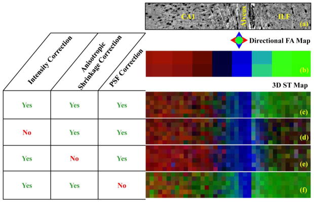
(a) An xy plane of the 3D montage. (b) Directional diffusion FA map. (c) A directional FA_ST map with all three corrections, (d) without intensity correction, (e) without anisotropic shrinkage correction, and (f) without PSF correction.

Structure tensor based image Analysis

The results of 3D structure tensor analysis using a Gaussian kernel with standard deviation (Eq. 3) of 2 μm, and an averaging neighborhood N (Eq. 4) of 37.5 μm × 37.5 μm × 12.5 μm in the x, y, and z directions, respectively, are shown in Fig. 6c. In a manner analogous to the directional FA map of Fig. 6b, red, blue, and green color intensities in Fig. 6c are scaled by the 3D structure tensor-derived factors ${FA}_{ST}{v}_{3,x}^2,{FA}_{ST}{v}_{3,y}^2$, and ${FA}_{ST}{v}_{3,z}^2$, respectively. Comparison of Figs. 6b and 6c reveals a strong similarity expected between the directions of the primary eigenvector of the diffusion tensor and the minor eigenvector of the 3D structure tensor. In particular, the boundary between CA1 (red voxels, Fig. 6b and c) and the alveus (blue voxels, Fig 6b and c), as well as the boundary between the alveus and the ILF (green voxels, Fig 6b and c) are coincident in the original DiI image and the directional FA and 3D structure tensor maps.

Directional 3D structure tensor maps shown in Fig. 6d–f illustrate the consequences of neglecting to implement the steps taken to remove artificially-introduced sources of 3D image anisotropy. In each of the Fig. 6d–f panels, all but one of the correction steps are applied, as indicated in the left side of the figure. If the z-dependent intensity bias is not corrected, systematic variation in image intensity will interfere with the ability to assign the direction of minimal intensity variation to the z-direction. As a result, the orientation of the structure tensor minor eigenvector is not co-linear with the z-axis, which leads to a discrepancy between the 3D structure tensor analysis and underlying tissue within structures oriented parallel to the z-axis such as the ILF (right side of Fig. 6d). Similarly, if anisotropic tissue shrinkage is not corrected, the calculated 3D structure tensor orientations will be inaccurate. As shown in Fig. 6e, preferential tissue shrinkage along the z-direction causes the ILF fibers to appear less anisotropic, and the direction of minimal image intensity variation is not co-linear with these fibers. Last, Fig. 6f illustrates the effects of omitting correction of PSF anisotropy. If image resolution is anisotropic, intensity variation will be minimal along the direction in which resolution is lowest. As shown in Fig. 6f, bias is present in the uncorrected image in which the 3D structure tensor minor eigenvectors largest component is found to be parallel to the z-direction within CA1 and parts of the alveus.

Quantitative comparisons between water diffusion anisotropy and anisotropy of the structure tensor are presented in figures 7 and 8. In Fig. 7, FA color maps (Fig. 7a–c) and grayscale FA maps (Fig. 7d–f) are shown for DTI data (Fig. 7a,d), and 3D structure tensor data, calculated using a Gaussian convolution kernel with a width of σ = 0.5 μm (Fig. 7b,e) and σ = 3 μm (Fig. 7c,f). As is evident in the FA color maps, the orientation of the structure tensor minor eigenvector remains constant over this range. Although close correspondence is observed between the structure tensor minor eigenvector and DTI primary eigenvector orientations throughout the field of view, there are regions of similarities as well as differences between FA_ST and FA. Within CA1 and the alveus, the same heterogeneous pattern is observable, in which anisotropy is lowest at the CA1/alveus border, and higher within neighboring gray and white matter regions. However, within the ILF, FA is uniformly high (0.7 to 0.8) whereas FA_ST is highest at the alveus/ILF border, and FA_ST decreases from approximately 0.75 at its highest value to approximately 0.5 deep within the ILF. In figures 7a–f, FA_ST and FA are observed to vary as a function of position along the horizontal direction (the “x”-direction, Fig. 7a), but FA_ST and FA are constant along the vertical direction. In Fig. 7g, FA_ST and FA values are averaged along the vertical direction, and the averaged FA_ST values are plotted for σ = 0.5 μm and σ = 3 μm, alongside FA values. The effect of Gaussian convolution kernel width is for FA_ST to increase slightly with σ.

Figure 7.

(a–c) Directional FA maps and (d–f) grayscale FA maps following DTI and 3D structure tensor analyses. (a) and (d) are d-MRI data, (b) and (e) are FA_ST with σ = 0.5 μm and (c) and (f) are FA_ST with σ = 3.0 μm. (g) FA (solid thick line) and FA_ST (dashed and dotted thin lines) values were averaged along the vertical (y) direction and plotted vs. position along the horizontal (x) direction.

Figure 8.

(a–e) Directional FA maps and (f–j) grayscale FA maps following DTI and 3D structure tensor analyses. FA_ST values were determined with neighborhood sizes of (b,g) 12.5×12.5×12.5 μm³, (c,h) 37.5×37.5×12.5 μm³, (d,i) 75×75×12.5 μm³, and (e,j) 112.5×112.5×12.5 μm³ with a Gaussian kernel width σ = 2.0 μm. (k) Average FA_ST values (thin lines) and FA values (thick line) are shown as a function of horizontal position in the hippocampal montage. (l) and (m) are correlation plots between FA_ST (ordinate) and FA (abscissa) with neighborhood size 12.5×12.5×12.5 μm in (l) and 112.5×112.5×12.5 μm (m).

The influence of the neighborhood size on FA_ST was examined as shown in figure 8. Color FA (Fig. 8b–e) and grayscale (Fig. 8g–j) FA_ST maps are shown for a range of neighborhood sizes, and these are compared to the DTI data shown in Fig. 8a and f. For all calculations, the Gaussian kernel width was σ = 2 μm, the neighborhood size in the z-direction was 12.5 μm, and the in-plane dimensions were 12.5×12.5 μm (Fig. 8b,g), 37.5×37.5 μm (Fig. 8c,h), 75×75 μm (Fig. 8d,i), and 112.5×112.5 μm (Fig. 8e,j). It was not possible to vary the neighborhood size in the z-direction due to the thickness of the tissue section. Average FA_ST values are shown as a function of horizontal position in Fig. 8k. As can be seen, within CA1 and alveus, FA_ST values approach DTI-derived FA as the neighborhood size approaches the voxel volume used in the d-MRI experiment. However, within the ILF, discrepancies are observed at all neighborhood sizes examined, in which FA_ST nearest the alveus/ILF border is highest, and FA_ST decreases with depth within ILF. The correlation between FA_ST and FA is directly compared in Fig. 8l (12.5×12.5×12.5 μm neighborhood size) and Fig. 8m (112.5×112.5×12.5 μm neighborhood size), in which data from CA1, alveus, and ILF, are color-coded red, blue, and green, respectively. For the smaller neighborhood size, the correlation between 3D structure tensor and DTI is poor. However, for CA1 and alveus voxels, the correlation between 3D structure tensor and DTI improves markedly with increased neighborhood size. Within the ILF, a persistent discrepancy between FA_ST and FA is observed, in which FA_ST is lower than FA within the deep ILF (right-most side of Fig 8k) regardless of neighborhood size. To explore this discrepancy in greater detail, individual eigenvalues of the structure tensor are plotted as a function of horizontal position specifically within the ILF in Fig. 9b. Throughout the ILF, the eigenvalue associated with lowest intensity variation (τ₃) is oriented in the through-plane direction and remains constant. In contrast, the largest structure tensor eigenvalue is associated with an eigenvector oriented in the left/right direction in Fig. 9a, and this eigenvalue varies from a relatively high value proximal to the alveus/ILF border to a lower value that approaches τ₂ deep within the ILF. Thus, reduced in-plane image intensity variation on the right side of the Fig. 9a compared to the left underlies the varying degrees of agreement between FA_ST and FA observed throughout the ILF.

Figure 9.

(a) Microscopic image of the ILF region of the hippocampal montage. (b) Each of the eigenvalues are averaged over the vertical (y) direction, and plotted as a function of the horizontal (x) direction.

DISCUSSION

With recent advances in tissue preparation methods (Kim et al., 2013; Kuwajima et al., 2013; Wu et al., 2014) and microscope configurations (Wu et al., 2013) designed to improve 3D light microscopy capabilities, 3D analyses for validating d-MRI findings will become increasingly powerful. Here, an extension of 2D structure tensor determinations to 3D is presented. The purpose of this work is to make structure tensor analyses possible in tissue sections that are not cut parallel to the orientation of underlying cellular structures. Quantitative anisotropy indices obtained from 2D structure tensor calculations depend on the angle between the sectioning plane and the structure tensor minor eigenvector. This dependence introduces a potential confound for 2D structure tensor analyses but the sectioning plane orientation does not influence 3D structure tensor calculations. The DiI immersion staining method used for this work was designed to non-specifically label membrane structures for purposes of d-MRI validation (Budde and Frank, 2012). Brain tissue from a nonhuman primate hippocampus and associated WM was used for implementing the method because it contains regions with three distinct groups of orthogonal fiber orientations. In addition, the cellular morphological characteristics of this structure are of functional significance, including the potential to reveal responses to environmental stimuli such as stress (Vestergaard-Poulsen et al., 2011).

In order to obtain 3D structure tensor orientations that resemble those of diffusion tensors in orientation-weighted FA maps, it was found that three operations were necessary to remove sources of 3D structure tensor anisotropy introduced by the confocal measurement system. As shown in Fig. 6, de-trending of the z-dependent intensity variation, correction for anisotropic tissue shrinkage, and application of a blurring filter in the x and y dimensions were each necessary. It is noted that the need for these steps arises from sectioning and confocal microscopy measurement through more than 100 μm of non-transparent tissue. Thus, in future work it may be possible to utilize optical clearing methods (Kuwajima et al., 2013) to enable the analysis of thicker and more transparent tissue sections. Such efforts may reduce or remove the need for the post-acquisition data processing steps described here.

Although the correction methods enabled structure tensor orientation maps to be generated that correspond to diffusion tensor orientations, differential results were observed between magnitudes of 3D structure tensor and diffusion tensor fractional anisotropy values. Within the CA1 GM and alveus, FA_ST was larger than FA for small neighborhood sizes, but as the neighborhood size was increased to approach the d-MRI voxel size, the CA1 and alveus FA_ST decreased toward the value of FA. Within the ILF however, FA_ST was more similar to FA near the alveus/ILF border than deep within the tract. This discrepancy was not resolved by changing the 3D structure tensor neighborhood size, and although differences between FA_ST and FA could not be assigned to any obvious structural/morphological characteristic within the ILF WM, inspection of the structure tensor eigenvalues revealed that differences in image intensity variation in x vs. y directions present near the alveus were absent in deep ILF tissue (Fig. 8b–e) which resulted in the observed FA_ST variation. Additional analyses were also performed in which the image derivatives I_x, I_y, and I_z were normalized by the length of the vector ∇I (data not shown). These analyses yielded a similar discrepancy between FA_ST and FA in the deep ILF but not at the alveus/ILF border, which indicates that heterogeneity in image gradient orientation, rather than the magnitude of the image derivatives, underlies the differential agreement between FA_ST and FA throughout the ILF. These differences between FA_ST and FA serve to emphasize the intrinsic differences between d-MRI and structure tensor analyses of DiI-stained tissue. Whereas d-MRI reveals anisotropy of water diffusion, the structure tensor analysis provides a measure of anisotropy in the variation in staining intensity. Several factors, such as axon diameter, myelin sheath thickness, packing density of stained fibers, and the spatial scale of each of these factors relative to the resolution of the light microscope images, could influence DiI staining intensity variation. Thus, in 3D structure tensor applications designed to validate quantitative diffusion MRI measurements and interpretations, fundamental differences in the techniques should be recognized as potential limitations in quantitative comparisons between d-MRI and 3D structure tensor results.

A number of methods have recently been described for using light microscopy to validate interpretations of d-MRI measurements in terms of cell morphology and intra-voxel fiber orientation dispersion (Budde and Frank, 2012; Choe et al., 2012; Flint et al., 2010; Hansen et al., 2011; Jespersen et al., 2012; Leergaard et al., 2010a). From these studies, two image analysis strategies have emerged. In the biophysical modeling strategy, manual (Dean et al., 2013; Leergaard et al., 2010a) or automatic (Jespersen et al., 2012) tracing is performed to construct models of neurons. These could in principle be used as boundary conditions for the diffusion equation in simulations, but in practice to date have been used in combination with simplifying assumptions to model diffusion restricted by cellular membranes (Jespersen et al., 2010; Jespersen et al., 2007; Jespersen et al., 2012; Kroenke et al., 2004). Advantages of this strategy stem from the fact that assumptions related to the connection between the d-MRI signal and cellular structural characteristics are made explicitly, which facilitates the interpretation of diffusion measurements in terms of cellular structure and morphology. The disadvantages of this approach are 1) that it relies on a staining method that selectively labels cells so that reconstructions can be performed, and this constraint can introduce bias in the set of cells that are labeled, and 2) that reconstructions are time consuming and operator dependent. The alternate method of d-MRI validation is the statistical/empirical strategy. In this approach, statistical quantities such as cell number or component volume fractions (Jespersen et al., 2010; Vestergaard-Poulsen et al., 2011), fiber orientation density metrics (Choe et al., 2012), or structure tensor metrics (Budde and Annese, 2013; Budde and Frank, 2012; Budde et al., 2011; Leigland et al., 2013) are compared to quantitative outcomes from d-MRI measurements. Although a disadvantage of this empirical strategy is that it relies on correlations between measured parameters rather than direct biophysical modeling, this can be offset by its flexibility and ease of implementation. Structure tensor measurements in particular have been demonstrated to be possible using a wide variety of staining techniques (Budde and Annese, 2013; Budde et al., 2011). Given the flexibility with regard to staining procedure, additional nonspecific fluorescent microscopy methods that do not rely on “exogenous probes,” such as imaging following glutaraldehyde fixation (Christensen et al., 2014), could likely further complement structure tensor analyses of DiI-immersion stained tissue.

An additional specific advantage of structure tensor analysis as a d-MRI validation tool is the ability to control the kernel size for calculating spatial derivatives, which is analogous to controlling the diffusion time in a d-MRI experiment, and the neighborhood size, which is analogous to controlling the d-MRI image resolution. For the tissue examined here, anisotropy in the 3D structure tensor did not change appreciably as the Gaussian kernel standard deviation ranged from 0.5 to 3 μm. In contrast, manipulation of the neighborhood size did influence FA_ST measurements in a predictable manner. In future work, biophysical modeling approaches could be incorporated into the empirical structure tensor analysis framework by replacing the spatial derivatives in Eqs. [1–2] with operations that more closely resemble the response of the d-MRI signal to molecular diffusion. Even as an empirical tool, however, structure tensor analysis has already demonstrated utility for validating d-MRI measurements, and it is hoped that generalization of this method to 3D will further contribute to its flexibility (Budde and Annese, 2013; Budde and Frank, 2012; Budde et al., 2011; Leigland et al., 2013).

CONCLUSION

Here we demonstrate the ability to perform 3D structure tensor analyses on confocal light microscopy data of DiI-stained primate hippocampal tissue. The advantage of 3D structure tensor analysis relative to 2D derives from the ability to characterize through-plane anisotropy, in a manner that is similar to MRI-based diffusion anisotropy measurements. It is envisioned this analysis will extend the utility of structure tensor-based validation analyses by removing the need to section tissue in a direction orthogonal to the primary direction of diffusion anisotropy, and by enabling the analysis of tissue in which primary diffusion directions of interest are oblique to a single 2D plane.

Highlights.

• Diffusion MRI (d-MRI) is an important neuroimaging modality that is in need of validation

• Structure tensor (ST) analysis of light microscopy data has been generalized from 2D to 3D

• 3D ST analysis can be performed independent of tissue sectioning plane orientation

• 3D ST analysis is implemented on confocal microscopy images of hippocampal tissue

• Agreement is observed for the 3 dominant tissue orientations present in the hippocampal sample

References

- Basser PJ, Pierpaoli C. Microstructural and physiological features of tissues elucidated by quantitative-diffusion-tensor MRI. Journal of Magnetic Resonance Series B. 1996;111:209–219. doi: 10.1006/jmrb.1996.0086. [DOI] [PubMed] [Google Scholar]
- Batchelor PG, Atkinson D, Hill DLG, Calamante F, Connelly A. Anisotropic noise propagation in diffusion tensor MRI sampling schemes. Magnetic Resonance in Medicine. 2003;49:1143–1151. doi: 10.1002/mrm.10491. [DOI] [PubMed] [Google Scholar]
- Beaulieu C. What makes diffusion anisotropic in the nervous system. Diffusion MRI: Theory, methods, and applications. 2011:92–109. [Google Scholar]
- Bozzali M, Cercignani M, Sormani MP, Comi G, Filippi M. Quantification of brain gray matter damage in different MS phenotypes by use of diffusion tensor MR imaging. American Journal of Neuroradiology. 2002;23:985–988. [PMC free article] [PubMed] [Google Scholar]
- Budde MD, Annese J. Quantification of anisotropy and fiber orientation in human brain histological sections. Frontiers in integrative neuroscience. 2013:7. doi: 10.3389/fnint.2013.00003. [DOI] [PMC free article] [PubMed] [Google Scholar]
- Budde MD, Frank JA. Examining brain microstructure using structure tensor analysis of histological sections. NeuroImage. 2012;63:1–10. doi: 10.1016/j.neuroimage.2012.06.042. [DOI] [PubMed] [Google Scholar]
- Budde MD, Janes L, Gold E, Turtzo LC, Frank JA. The contribution of gliosis to diffusion tensor anisotropy and tractography following traumatic brain injury: validation in the rat using Fourier analysis of stained tissue sections. Brain. 2011;134:2248–2260. doi: 10.1093/brain/awr161. [DOI] [PMC free article] [PubMed] [Google Scholar]
- Choe AS, Stepniewska I, Colvin DC, Ding Z, Anderson AW. Validation of diffusion tensor MRI in the central nervous system using light microscopy: quantitative comparison of fiber properties. NMR in Biomedicine. 2012;25:900–908. doi: 10.1002/nbm.1810. [DOI] [PMC free article] [PubMed] [Google Scholar]
- Christensen PC, Brideau C, Poon KWC, Doring A, Young VW, Stys PK. High-resolution fluorescence microscopy of myelin without exogenous probes. NeuroImage. 2014;87:42–54. doi: 10.1016/j.neuroimage.2013.10.050. [DOI] [PubMed] [Google Scholar]
- Cole RW, Jinadasa T, Brown CM. Measuring and interpreting point spread functions to determine confocal microscope resolution and ensure quality control. NATURE PROTOCOLS. 2011;6:1929–1941. doi: 10.1038/nprot.2011.407. [DOI] [PubMed] [Google Scholar]
- D’Arceuil H, Crespigny Ad. Diffusion imaging in gray matter. In: Jones DK, editor. Diffusion MRI: Theory, methods, and applications. Oxford University Press; 2010. pp. 647–660. [Google Scholar]
- Dauguet J, Peled S, Berezovskii V, Delzescaux T, Warfield SK, Born R, Westin CF. Comparison of fiber tracts derived from in-vivo DTI tractography with 3D histological neural tract tracer reconstruction on a macaque brain. NeuroImage. 2007;37:530–538. doi: 10.1016/j.neuroimage.2007.04.067. [DOI] [PubMed] [Google Scholar]
- Daunais JB, Kraft RA, Davenport AT, Burnett EJ, Maxey VM, Szeliga KT, Rau AR, Flory GS, Hemby SE, Kroenke CD. MRI-guided dissection of the nonhuman primate brain: a case study. Methods. 2010;50:199–204. doi: 10.1016/j.ymeth.2009.03.023. [DOI] [PMC free article] [PubMed] [Google Scholar]
- Dean JM, McClendon E, Hansen K, Azimi-Zonooz A, Chen K, Riddle A, Gong X, Sharifnia E, Hagen M, Ahmad T, Leigland LA, Hohimer AR, Kroenke CD, Back SA. Prenatal cerebral ischemia disrupts MRI-defined cortical microstructure through disturbances in neuronal arborization. Science translational medicine. 2013;5:168ra167–168ra167. doi: 10.1126/scitranslmed.3004669. [DOI] [PMC free article] [PubMed] [Google Scholar]
- Flint JJ, Hansen B, Fey M, Schmidig D, King MA, Vestergaard-Poulsen P, Blackband SJ. Cellular-level diffusion tensor microscopy and fiber tracking in mammalian nervous tissue with direct histological correlation. NeuroImage. 2010;52:556–561. doi: 10.1016/j.neuroimage.2010.04.031. [DOI] [PMC free article] [PubMed] [Google Scholar]
- Gao Y, Choe AS, Stepniewska I, Li X, Avison MJ, Anderson AW. Validation of DTI Tractography-Based Measures of Primary Motor Area Connectivity in the Squirrel Monkey Brain. PLOS One. 2013;8:e75065. doi: 10.1371/journal.pone.0075065. [DOI] [PMC free article] [PubMed] [Google Scholar]
- Hansen B, Flint JJ, Heon-Lee C, Fey M, Vincent F, King MA, Vestergaard-Poulsen P, Blackband SJ. Diffusion tensor microscopy in human nervous tissue with quantitative correlation based on direct histological comparison. NeuroImage. 2011 doi: 10.1016/j.neuroimage.2011.04.052. [DOI] [PMC free article] [PubMed] [Google Scholar]
- Jespersen SN, Bjarkam CR, Nyengaard JR, Chakravarty MM, Hansen B, Vosegaard T, Ostergaard L, Yablonskiy DA. Neurite density from magnetic resonance diffusion measurements at ultrahigh field: comparison with light microscopy and electron microscopy. NeuroImage. 2010;49:205–216. doi: 10.1016/j.neuroimage.2009.08.053. [DOI] [PMC free article] [PubMed] [Google Scholar]
- Jespersen SN, Kroenke CD, Østergaard L, Ackerman JH, Yablonskiy DA. Modeling dendrite density from magnetic resonance diffusion measurements. NeuroImage. 2007;34:1473–1486. doi: 10.1016/j.neuroimage.2006.10.037. [DOI] [PubMed] [Google Scholar]
- Jespersen SN, Leigland LA, Cornea A, Kroenke CD. Determination of axonal and dendritic orientation distributions within the developing cerebral cortex by diffusion tensor imaging. IEEE Transactions on Medical Imaging. 2012;31:16–32. doi: 10.1109/TMI.2011.2162099. [DOI] [PMC free article] [PubMed] [Google Scholar]
- Jones DK, Horsfield MA, Simmons A. Optimal strategies for measuring diffusion in anisotropic systems by magnetic resonance imaging. Magnetic Resonanace in Medicine. 1999;42:515–525. [PubMed] [Google Scholar]
- Jones DK, Knösche TR, Turner R. White matter integrity, fiber count, and other fallacies: the do’s and don’ts of diffusion MRI. NeuroImage. 2013;73:239–254. doi: 10.1016/j.neuroimage.2012.06.081. [DOI] [PubMed] [Google Scholar]
- Kim SY, Chung K, Deisseroth K. Light microscopy mapping of connections in the intact brain. Trends in cognitive sciences. 2013;17:596–599. doi: 10.1016/j.tics.2013.10.005. [DOI] [PubMed] [Google Scholar]
- Kroenke CD, Ackerman JJH, Yablonskiy DA. On the nature of the NAA diffusion attenuated MR signal in the central nervous system. Magnetic Resonanace in Medicine. 2004;52:1052–1059. doi: 10.1002/mrm.20260. [DOI] [PubMed] [Google Scholar]
- Kuwajima T, Sitko AA, Bhansali P, Jurgens C, Guido W, Mason C. ClearT: a detergent-and solvent-free clearing method for neuronal and non-neuronal tissue. Development. 2013;140:1364–1368. doi: 10.1242/dev.091844. [DOI] [PMC free article] [PubMed] [Google Scholar]
- Le Bihan D. Looking into the functional architecture of the brain with diffusion MRI. Nature Reviews Neuroscience. 2003;4:469–480. doi: 10.1038/nrn1119. [DOI] [PubMed] [Google Scholar]
- Leergaard TB, Nathan SW, de Crespigny A, Ingeborg B, D’Arceuil H, Bjaalie JG, Dale MA. Quantitative histological validation of diffusion MRI fiber orientation distributions in the rat brain. PLOS One. 2010a;5:e8595. doi: 10.1371/journal.pone.0008595. [DOI] [PMC free article] [PubMed] [Google Scholar]
- Leergaard TB, SWN, de Crespigny A, Ingeborg B, D’Arceuil H, Bjaalie JG, Dale MA. Quantitative histological validation of diffusion MRI fiber orientation distributions in the rat brain. PloS one. 2010b;5:e8595. doi: 10.1371/journal.pone.0008595. [DOI] [PMC free article] [PubMed] [Google Scholar]
- Leigland LA, Budde MD, Cornea A, Kroenke CD. Diffusion MRI of the developing cerebral cortical gray matter can be used to detect abnormalities in tissue microstructure associated with fetal ethanol exposure. NeuroImage. 2013;83:1081–1087. doi: 10.1016/j.neuroimage.2013.07.068. [DOI] [PMC free article] [PubMed] [Google Scholar]
- Matthews C, Cordelières FP. MetroloJ: an ImageJ plugin to help monitor microscopes’ health. ImageJ User and Developer Conference; Mondorf-les-Bains, Luxembourg. 2010. [Google Scholar]
- Mori S, Wakana S, Van Zijl PCM, Nagae-Poetscher LM. MRI atlas of human white matter. 2005. [DOI] [PubMed] [Google Scholar]
- NIH. Guide for the care and use of laboratory animals. The National Academics Press; Washington, D.C: 1987. pp. 86–23. [Google Scholar]
- Novikov DS, Jensen JH, Helpern JA, Fieremans E. Revealing mesoscopic structural universality with diffusion. Proc Natl Acad Sci U S A. 2014;111:5088–5093. doi: 10.1073/pnas.1316944111. [DOI] [PMC free article] [PubMed] [Google Scholar]
- Parekh R, Ascoli GA. Neuronal morphology goes digital: a research hub for cellular and system neuroscience. Neuron. 2013;77:1017–1038. doi: 10.1016/j.neuron.2013.03.008. [DOI] [PMC free article] [PubMed] [Google Scholar]
- Shepherd TM, Özarslan E, King MA, Mareci TH, Blackband SJ. Structural insights from high-resolution diffusion tensor imaging and tractography of the isolated rat hippocampus. Neuroimage. 2006;32:1499–1509. doi: 10.1016/j.neuroimage.2006.04.210. [DOI] [PubMed] [Google Scholar]
- Vestergaard-Poulsen P, Wegener G, Hansen B, Bjarkam CR, Blackband SJ, Nielsen NC, Jespersen SN. Diffusion-weighted MRI and quantitative biophysical modeling of hippocampal neurite loss in chronic stress. PLOS One. 2011;6:e20653. doi: 10.1371/journal.pone.0020653. [DOI] [PMC free article] [PubMed] [Google Scholar]
- Wang Y, Wang Q, Haldar JP, Yeh FC, Xie M, Sun P, Tu TW, Trinkaus K, Klein RS, Cross AH. Quantification of increased cellularity during inflammatory demyelination. Brain. 2011;134:3590–3601. doi: 10.1093/brain/awr307. [DOI] [PMC free article] [PubMed] [Google Scholar]
- Wedeen VJ, Wang RP, Schmahmann JD, Benner T, Tseng WYI, Dai G, Pandya DN, Hagmann P, D’Arceuil H, de Crespigny AJ. Diffusion spectrum magnetic resonance imaging (DSI) tractography of crossing fibers. NeuroImage. 2008;41:1267–1277. doi: 10.1016/j.neuroimage.2008.03.036. [DOI] [PubMed] [Google Scholar]
- Wu J, He Y, Yang Z, Guo C, Luo Q, Zhou W, Chen S, Li A, Xiong B, Jiang T. 3D BrainCV: Simultaneous visualization and analysis of cells and capillaries in a whole mouse brain with one-micron voxel resolution. NeuroImage. 2014;87:199–208. doi: 10.1016/j.neuroimage.2013.10.036. [DOI] [PubMed] [Google Scholar]
- Wu Y, Wawrzusin P, Senseney J, Fischer RS, Christensen R, Santella A, York AG, Winter PW, Waterman CM, Bao Z. Spatially isotropic four-dimensional imaging with dual-view plane illumination microscopy. Nature biotechnology. 2013;31:1032–1038. doi: 10.1038/nbt.2713. [DOI] [PMC free article] [PubMed] [Google Scholar]
- Zhang J, van Zijl P, Mori S. Three-dimensional diffusion tensor magnetic resonance microimaging of adult mouse brain and hippocampus. NeuroImage. 2002;15:892–901. doi: 10.1006/nimg.2001.1012. [DOI] [PubMed] [Google Scholar]