

Abstract
Decision-making systems trained on structural Magnetic Resonance Imaging (MRI) data of subjects affected by the Alzheimer’s disease (AD) and healthy controls (CTRL) are becoming widespread prognostic tools for subjects with Mild Cognitive Impairment (MCI). This study compares the performance of three classification methods based on Support Vector Machines (SVMs), using as initial sets of brain voxels (i.e. features): 1) the segmented grey matter (GM); 2) regions of interest (ROIs) by voxel-wise t-test filtering; 3) parceled ROIs, according to prior knowledge. The recursive feature elimination (RFE) is applied in all cases in order to investigate whether feature reduction improves the classification accuracy. We analyzed more than 600 ADNI subjects, training the SVMs on the AD/CTRL dataset, and evaluating them on a trial MCI dataset. The classification performance, evaluated as the Area Under the Receiver Operating Characteristic (ROC) Curve (AUC), reaches AUC=(88.9±0.5)% in 20-fold cross-validation on the AD/CTRL dataset, when the GM is classified as a whole. The highest discrimination accuracy between MCI converters and non-converters is achieved when the SVM-RFE is applied to the whole GM: with AUC reaching (70.7±0.9)%, it outperforms both ROI-based approaches in predicting the AD conversion.
Keywords: Alzheimer’s disease, Mild Cognitive Impairment, Classification, MRI, Support Vector Machine
Introduction
Diagnostic early markers of Alzheimer’s disease (AD) are widely investigated in order to aid researchers and clinicians in the validation of the effectiveness of new AD treatments, while limiting the duration and cost of clinical trials [1]. Brain atrophy and its evolution are recognized key neuroimaging biomarkers of the AD progression [2–9].
Brain scans acquired with structural Magnetic Resonance Imaging (MRI) are suitable for quantitative evaluation of brain atrophy; moreover, image analysis algorithms can process these in order to extract useful information and carry out both single-subject analyses and between-group comparisons.
Machine-learning techniques applied to MRI images are increasingly spreading tools that extract information from data and can predict the pathology progression [10,11]. The introduction of pattern classification and computer vision methods in the neuroimaging field is due to Lao et al. [12]. In order to develop an accurate predictor of pathology from a set of volumetric images, the authors highlighted the limitations of voxel-based morphometric methods and the potentiality of Support Vector Machine (SVM)-based decisional systems.
Classification approaches can be particularly useful in studies on the AD pathology, as they predict the conversion to AD of those subjects referred to as affected by Mild Cognitive Impairment (MCI), a transitional state between normal aging and dementia [13].
Several machine-learning techniques have been implemented so far in neuroimaging studies on AD, such as Principal Component Analysis (PCA) and Linear Discrimination Analysis (LDA) [14,15], SVM [16–21], logistic regression [22], the combination of information extracted from different diagnostic modalities and their classification with SVM [23], with an automatic learning framework [24], or by combining multiple weak classifiers to achieve more accurate and robust results [25]. Many research groups investigating the AD pathology in recent years developed and validated their analyses on data samples provided by the Alzheimer’s Disease Neuroimaging Initiative (ADNI) [15,19–26], as reported in the extensive review carried out by the Principal Investigator on the ADNI initiative Michael W. Weiner and colleagues [27].
Recent studies by Cuingnet et al. [20] and Chu et al. [21] on ADNI data were focused on a comparison between whole-brain classification methods and Region Of Interest (ROI)-based approaches, all coupled to feature reduction methods, required by the huge input data size. Both studies concluded that feature selection does not improve the classification accuracy and that whole-brain methods outperform ROI-based ones, unless the ROIs are chosen according to a prior knowledge of the underlying disease. A recent study by Adaszewski et al. [28] on longitudinal data of AD, MCI and control (CTRL) subjects, reports that feature selection improves the classification accuracy at early MCI stages, whereas at a later stage whole-brain methods are superior.
We focused our analysis on a comparison between three different methods, in order to select the initial sets of brain voxels to analyze with SVM classifiers. In particular, they are defined as: 1) the segmented grey matter (GM), referred as whole-GM classification; 2) the regions of interest (ROIs), obtained by the voxel-based morphometry (VBM) analysis, i.e. voxel-wise t-test filtering, referred as VBM-ROI classification; 3) the parceled ROIs, chosen according to prior knowledge on the brain involvement in the AD pathology, referred as LONI-ROI classification, as the parcellation of the anatomical regions is performed according to LONI Probabilistic Brain Atlas (LPBA40) [29].
The recursive feature elimination (RFE) method [30] has been implemented in our whole-GM analysis both in order to reduce the data size, and to localize the brain regions that are more involved in the AD pathology. The same approach has been applied also to the VBM-ROI and LONI-ROI classification, so as to evaluate the SVM-RFE potentiality in enhancing the classification performance. Methods 1) and 2), complemented with the RFE procedure, can be considered as data driven approaches, where different criteria to select the initial set of features are implemented (whole-GM vs. t-test filtered ROIs). They are compared to 3) a prior-knowledge based analysis, where the right and left hippocampi and parahippocampal gyrii are considered as relevant ROIs in the AD pathology.
All the approaches are compared in terms of their ability in correctly distinguishing AD from CTRL subjects and making accurate conversion predictions on the MCI population. The relative performances are compared in term of the Area Under the Receiver Operating Characteristic (ROC) Curve (AUC), evaluated within cross-validation protocols. The meaning of AUC has been proved to be the probability that a random pair of positive/diseased and negative/non-diseased individuals would be correctly identified by the diagnostic test [31].
The analysis is carried out on a MRI dataset extracted from the publicly available ADNI collection.
This paper is structured as follows: a description of the MRI data source and its characteristics is provided; then, a methodological overview for the VBM analysis and the machine-learning SVM procedure is given; the implementation of decisional systems in the whole-GM, VBM-ROI and LONI-ROI analysis is described, and finally results are discussed and compared to other methods.
Materials and Methods
The ADNI data sample
Data used in the preparation of this article were obtained from the Alzheimer’s Disease Neuroimaging Initiative (ADNI) database (adni.loni.ucla.edu). The ADNI was launched in 2003 by the National Institute on Aging (NIA), the National Institute of Biomedical Imaging and Bioengineering (NIBIB), the Food and Drug Administration (FDA), private pharmaceutical companies and non-profit organizations, as a $60 million, 5-year public-private partnership. The primary goal of ADNI has been to test whether serial MRI, positron emission tomography (PET), other biological markers and clinical and neuropsychological assessment can be combined to measure the progression of mild cognitive impairment (MCI) and early Alzheimer’s disease (AD). Determination of sensitive and specific markers of very early AD progression is intended to aid researchers and clinicians to develop new treatments and monitor their effectiveness, as well as lessen the time and cost of clinical trials.
The Principal Investigator of this initiative is Michael W. Weiner, MD, VA Medical Center and University of California – San Francisco. ADNI is the result of efforts of many co-investigators from a broad range of academic institutions and private corporations, and subjects have been recruited from over 50 sites across the U.S. and Canada. The initial goal of ADNI was to recruit 800 adults, aged 55 to 90, to participate in the research, approximately 200 cognitively normal older individuals to be followed for 3 years, 400 people with MCI to be followed for 3 years and 200 people with early AD to be followed for 2 years. Up-to-date information is available on www.adni-info.org.
The analysis reported in this paper has been carried out on the structural MRI data of 635 subjects extracted from the ADNI database. The statistical data of these subjects are summarized in Table 1. The subjects have been divided into two categories: a training/testing and a trial set. The training/testing set consisted of 333 age and sex-matched subjects, namely 189 CTRL and 144 AD. The trial set consisted of 302 MCI subjects, among which 136 converted to AD in a time frame of 2 years from the baseline scans. These subjects were selected from the larger ADNI data on the basis of the availability of baseline and at least 2 years information. Moreover, training subjects were chosen if confirmed to be CTRL/AD at follow-up assessment. The data samples considered in this work are the same analyzed in the paper by Chincarini et al. [19].
Table 1.
Demographic and mini mental state examination (MMSE) score of the data samples.
| Cohort | Sample size | Age | Gender (M/F) | MMSE |
|---|---|---|---|---|
| CTRL | 189 | 76.6 ± 5.1 | 95/95 | 29.1 ± 0.9 |
|
|
||||
| MCI-NC | 166 | 75.7 ± 7.3 | 106/60 | 27.2 ± 2.4 |
|
|
||||
| MCI-C | 136 | 75.1 ± 7.1 | 80/56 | 25.2 ± 2.7 |
|
|
||||
| AD | 144 | 75.5 ± 7.5 | 78/66 | 22.2 ± 3.3 |
MRI acquisition and preprocessing
The MRI ADNI data were acquired with 1.5 T scanners. Data were collected across a variety of scanners. Up-to-date information on ADNI eligibility criteria and protocols is available on http://www.adni-info.org. Raw NIFTI-converted MRI scans were downloaded from the ADNI site, automatically reviewed by signal-to-noise statistics for quality, and processed with a wavelet based noise-filtering algorithm to improve signal-to-noise ratio and image uniformity across different sites [19]. Denoised scans were registered onto the Montreal Neurological Institute (MNI) reference [32] with a 12-parameter affine registration and resampled onto a 1-mm3 isotropic grid. Images were then intensity-normalized as reported in Chincarini et al. [19] to achieve good histogram equalization among images coming from different scanners, while ensuring that the average gray levels of the three main cerebral matter contributions are mapped onto those of the MNI reference.
Voxel-based morphometry (VBM) preprocessing
We conducted a voxel-based morphometry (VBM) study [33] in order to investigate the differences in the regional volumes of grey matter (GM) between the AD and CTRL groups and between the MCI-C and MCI-NC groups, respectively. The T1-weighted volumetric images were analyzed with the SPM8 package (Statistical Parametric Mapping, Wellcome Department of Imaging Neuroscience, London, UK, http://www.fil.ion.ucl.ac.uk/spm), using the VBM protocol with modulation. We implemented the Diffeomorphic Anatomical Registration using Exponentiated Lie algebra (DARTEL) algorithm [34]. A diffeomorphic warping is implemented to achieve an accurate inter-subject registration with an improved realignment of small inner structures [35] and to generate a study-specific template. The VBM preprocessing was applied as follows: (1) SPM segmentation of brain tissues, i.e. grey matter (GM), white matter (WM) and cerebrospinal fluid (CSF), using the New Segment toolbox, which extends the segmentation procedure described in [36]; (2) importing the parameter files produced by the tissue segmentation in the DARTEL procedure [34] to generate a study-specific template and the deformation fields that warp the segmented tissues of each subjects to the DARTEL template; (3) affine transformation to the MNI space of the DARTEL template and of the segmented brain tissues previously aligned to the DARTEL template according to the generated deformation fields; (4) standard smoothing with isotropic Gaussian kernel. After the preprocessing, we obtained smoothed modulated normalized data (in the MNI space) to be used for the statistical analysis. The modulation operation is fundamental to render the final VBM statistics reflecting the local volume differences in tissue segments [33]. Modulation allows compensating for the effect of spatial warping that causes volume changes, so that the total amount of grey matter in the modulated images remains the same as it would be in the original images. The modulated GM segments thus need to be corrected for total intracranial volume to take into account brain size variability.
VBM statistical analysis
The regional GM volumes were compared between the AD/CTRL and the MCI-C/MCI-NC samples using the VBM-DARTEL analysis. The normalized modulated and smoothed GM image segments in each group were entered into a voxel-wise two-sample t-test analysis in SPM8. The conventional VBM analysis was employed using the stringent significance threshold p<0.05, family-wise error rate (FWE) corrected. An absolute threshold mask of 0.1 on GM was used to avoid possible edge effects around the border between GM and WM. Age, gender and the Total Intracranial Volume (TIV), computed as the sum of the SPM segmented GM, WM, and CSF were entered as covariates in the statistical analysis.
Multivariate analysis with Support Vector Machines (SVM)
We followed the classification approach with SVM proposed in Klöppel et al. [16] and in Ecker et al. [37]. As opposed to the mass-univariate VBM analysis, the pattern recognition techniques, e.g. SVMs, are multivariate and make use of specific inter-regional dependencies to help categorize scans [12,17].
An SVM [38] is a supervised binary classification method, i.e. it requires a training set, used to learn the differences between the two groups, and a validation set to quantify the classification performance on previously unseen data (see the schematic flowchart in Figure 1). In our analysis, each image is treated as a point in the high dimensional RN space, where the space dimension N is equal to the number of features/voxels in the considered ROI.
Figure 1.

Schematic representation of the SVM training on the AD/CTRL sample and the SVM validation on the MCI sample.
The SVM inputs are feature vectors, the sequence of the voxel intensity values of the ROI. The feature vectors belonging either to the category of patients and controls are labeled with “1” and “−1”, respectively. The trained SVM classifier maps the RN space into R, by assigning to the newly examined cases a one-dimensional (or binary) output. As the number of features/voxels can be very high especially when the whole GM is the ROI to classify, whereas the number of subjects considered in this study is limited to few hundreds, we considered only linear-kernel SVMs to avoid the risk of overfitting data. Training an SVM is a minimization problem where the largest-margin hyperplane allowing for an optimal separation of the training examples is identified. The separating hyperplane is defined by a weight vector and an offset, w • x + b = 0, where the weight vector w is a linear combination of the support vectors and it is normal to the hyperplane. During the SVM training a free parameter has to be set, the c value, that controls the trade-off between having zero training errors and allowing for misclassifications. The c value has been heuristically estimated in our analysis.
The SVM is trained according to the 20-fold cross-validation (20f-CV) technique. The data are partitioned in 20 folds; one of them is retained as validation data while the others are used to train the classifier. The process is repeated 20 times, i.e. until each subsample is used once as validation set. We used in this study the SVM-Light software package [39,40] (http://svmlight.joachims.org/).
The classification performance is evaluated through the Receiver Operating Characteristic (ROC) curve [41], where the sensitivity (true positive rate, i.e. the percentage of pathological subjects correctly classified) is plotted against the false positive rate (i.e. the percentage of misclassified control subjects). Different ROC curves are compared to each other in terms of the estimated AUC.
The initial selection of brain regions for the three SVM classifications we carried out was operated as follows:
Whole-GM classification. We consider as input to the SVM classifier the whole GM segmented volume obtained from the standardized and automated SPM preprocessing [16,37].
VBM-ROI classification. The ROIs that reached the statistical significance in the VBM analysis (p<0.05, FWE corrected) were used as data-driven reduced input to the SVM classifier.
LONI-ROI classification. The 1) and 2) voxel selection methods are complemented with a prior-knowledge based approach, where brain regions that encode interesting information for the AD pathology are selected on the basis of previous studies [2–4]. Usually Neuroradiologists are asked to manually identify the brain regions to be considered. As an alternative, atlas-based parcellation can be implemented to select anatomical regions in a more automated and reproducible way. In the present analysis we defined the ROIs according to the LONI Probabilistic Brain Atlas [29] (http://www.loni.ucla.edu.Atlases/LPBA40). In particular, brain regions where neurodegeneration is expected in AD have been chosen, i.e. the right and left hippocampi and the parahippocampal gyrii.
Discrimination maps and Recursive Feature Elimination (SVM-RFE)
The implementation of a linear-kernel SVM allows a direct extraction of the weight vector w as an image, which is referred to as discrimination map. The w vector, which is normal to the separating hyperplane and indicates the direction along which the images of the two groups differ most, can be used to generate a map of the most discriminating voxels in the images. As the intensity value reported in each voxel of the considered input images is proportional to the amount of GM in that specific location (the modulation option has been selected in the SPM segmentation), a higher/lower value in the discrimination map indicates that patients have higher/lower GM volume in that specific location with respect to controls.
In order to identify the voxels with the highest discriminating power, we implemented the SVM recursive feature elimination (SVM-RFE) procedure [30,42]. The SVM-RFE is a feature-selection technique that iteratively eliminates features/voxels from the data set, in order to remove as many non-informative features as possible, while retaining features that carry discriminative information. A new SVM classifier is trained at each iteration, thus a new weight map is generated. The selected feature-ranking criterion is the absolute value of each weight vector component |wi|. The features/voxels are iteratively excluded from the dataset with the aim of removing as many non-informative voxels as possible (low |wi|), while retaining those encoding the discriminative information (high |wi|).
The SVM-RFE algorithm is implemented in this study to estimate the SVM classification performance as a function of the number of GM voxels retained as input to the SVM. At each operative point of this curve the discrimination maps can be visualized to localize the set of voxels that encode the between-group discriminant information.
Prediction on the outcome of Mild Cognitive Impairment (MCI) subjects
The SVM-based method we present in this paper is able to provide single-subject classification, i.e. once an SVM classifier is trained on a learning dataset, it can be applied on previously unseen data and give a prediction on its class membership. In our analysis the SVMs, trained and validated on the AD/CTRL data sample, are evaluated on a completely independent validation set, constituted by MCI subjects. Also in this case the classifier performance is evaluated using the AUC as figure of merit.
Correlation between SVM test margin and cognitive decline
When attempting to set up a useful imaging biomarker, sensitive to the cognitive decline of patients with AD, it is important to test for correlation with the mini mental state examination (MMSE) score [1]. We studied the correlation between the distance of each data point from the SVM optimal hyperplane (we will refer to as the test margin) and the MMSE score of each subject using the Spearman’s rank correlation coefficient ρ [43].
Results
VBM results
Significant volumetric between-group differences have been found in the AD/CTRL sample with Gaussian smoothing scale s = 3 mm. By contrast, no significant between-group difference has been detected in the MCI-C/MCI-NC analysis at any considered smoothing scale (s = 3, 6, 8 mm). The areas of brain atrophy detected by VBM are shown in Figure 2, where the t statistics of the significantly different areas (p< 0.05, FWE corrected) is overlaid on a series of axial views of a representative T1 MRI of a single-subject. The effect is localized in the medial temporal lobe (MTL), as expected. The VBM cluster coordinates in the MNI reference space and in the standard Talairach and Tournoux space [44] (the conversion being performed with the Talairach Client [45,46]), beside the anatomical description of the corresponding brain areas, are reported in Table 2.
Figure 2.

Significant regions detected in the AD vs. CTRL VBM statistical analysis (colored regions reporting the t statistics), overlaid on a representative single-subject T1-weighted MRI (a sequence of axial views is displayed).
Table 2.
Anatomical structures detected in the AD vs. CTRL VBM analysis (data smoothed with s = 3 mm). These regions are visible in Figure 2.
| Cluster extent (voxels) | MNI coordinates | Talairach coordinates | Brain region localization | ||||||
|---|---|---|---|---|---|---|---|---|---|
| 2646 | −22 | −6 | −21 | −21 | −5 | −16 | LC | Limbic Lobe | Parahippocampal Gyrus, Amygdala |
| 2892 | 21 | −4 | −18 | 19 | −4 | −12 | RC | Limbic Lobe | Parahippocampal Gyrus, Amygdala |
| 62 | −16 | −39 | 1 | −16 | −38 | 1 | LC | Limbic Lobe | Parahippocampal Gyrus, BA27 |
| 57 | 18 | −36 | 1 | 16 | −35 | 2 | RC | Limbic Lobe | Parahippocampal Gyrus, BA27 |
| 158 | 56 | −19 | −8 | 51 | −19 | −4 | RC | Temporal Lobe | Superior Temporal Gyrus, BA22 |
Abbreviations: LC/RC, Left/Right Cerebrum; BA, Brodmann area.
SVM classification, SVM-RFE and discrimination maps
1) Whole-GM classification
The SVMs have been trained on the AD/CTRL sample according to the 20f-CV protocol and validated on the MCI cohort. In this paper we address a classification problem where the input is a vector that we call a pattern of n components, which we call features. Thus, a pattern is generated for each subject of our dataset, and the n features of each input vector are the voxel intensity values of the GM of each subject. It happens that the number of features/voxels is very large (about 6.5×10⁵), whereas the number of patterns in the training dataset is limited to about 300. The linear-kernel SVM demonstrated to be able to handle such disproportion between the number of weights to be estimated and the training examples.
The classification error due to the random partitioning of data into the train and test samples was estimated by repeating the 20f-CV procedure ten times and evaluating the corresponding average AUC and its standard deviation (SD). As shown in Figure 3, the discrimination performance of SVMs trained with all features/voxels of the GM segments is equal to AUC = (88.9±0.5)% on the AD/CTRL sample whereas it falls to AUC = (67.8±0.5)% on the MCI cohort.
Figure 3.
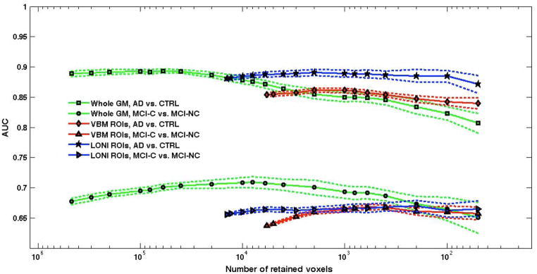
SVM-RFE of whole-GM, VBM-ROI and LONI ROI analyses. The SVM training and testing is performed on the AD/CTRL sample in 20f-CV; an independent validation is carried out on the MCI-C/MCI-NC sample. The average values obtained over 10 repetitions of 20f-CV are shown; the bands around the average curves correspond to two standard deviations.
The SVM-RFE procedure has been applied and the corresponding AUC variation as a function of the number of retained voxels is shown in Figure 3. The dotted lines above and below the curve highlight the average (AUC ± SD) band.
It can be noticed that, whereas the highest AUC values in the AD/CTRL discrimination are obtained when a large number of GM voxels are retained for the classification, the performance sensibly decreases when retaining less than 10000 voxels. By contrast, the trend of AUC in the MCI-C/MCI-NC SVM-RFE classification is completely different. We remind that the MCI cohort is used only as validation sample, i.e. the SVM classifiers trained on the AD/CTRL data are evaluated on the MCI cases, which did not influence the training process. The reduction in the number of retained voxels leads in this case to a slight optimization of the classification performance, up to AUC = (70.9±0.9)%, obtained with 8000 retained voxels.
2) VBM-ROI classification
The SVM classifier was trained with the grey level information encoded in the ROI identified by the VBM statistical analysis (see Sec. VBM results). About 6×10³ voxels were significantly different in the AD vs. CTRL statistical comparison. The SVM classification, according to the 20f-CV protocol repeated ten times, achieved AUC = (85.4±0.3)% in the discrimination between AD and CTRL subjects. The validation performance on the MCI dataset was less effective, with AUC = (63.7±0.2)%.
In order to optimize the discrimination performance, the SVM-RFE procedure has been applied also in this case. The behavior of AUC as a function of the number of retained voxels is shown in Figure 3 for both the AD/CTRL data and the validation cohort of the MCI-C/MCI-NC subjects. It can be noticed that despite the SVM-RFE procedure leads in this case to a tiny improvement in the classification performance in both the AD/CTRL and MCI-C/MCI-NC classification, in the latter case the AUC values remain well below the 70%.
3) LONI-ROI classification
The hippocampus and parahippocampal gyrus ROIs extracted from the LONI Probabilistic Brain Atlas were coregistered to our images and resliced to be used as masks to the segmented GM of our data sample. The resulting LONI-ROI dataset consisted of vectors of about 14×103 features, whose SVM classification provided AUC = (88.1±0.3)% on the AD/CTRL sample and AUC = (65.6±0.3)% on the MCI cohort. As shown in Figure 3, the SVM-RFE procedure has almost no effect on the classification performance.
Global vs. local approaches and discrimination information
A direct comparison between the classification performance of the whole-GM and the ROI-based methods is shown in Figure 3, which highlights two main results.
Before the RFE procedure is applied the whole-GM classification can be directly compared with t-test filtering (VBM-ROI) and prior-knowledge based method. The whole-GM classification outperforms both the ROI-based methods, especially in the prediction of the MCI outcome.
If the RFE is applied to all three datasets, the following considerations hold: i) the LONI-ROI approach shows similar performance to the whole-GM method in AD vs. CTRL classification, even when classifying only with a few hundreds voxels, but its classification accuracy on MCI subjects is not fully satisfactory; ii) the restrictive choice of classifying only the t-test filtered ROIs leads to a limited classification accuracy on both the AD/CTRL and the MCI samples; iii) the RFE applied to the whole-GM data maximizes the performance in MCI outcome prediction.
The AUC values obtained in the whole-GM SVM-RFE analysis considering 6000 retained voxels (corresponding approximately to the VBM ROI size) on the AD/CTRL and on the MCI-C/MCI-NC samples correspond to the areas under the ROC curves shown in Figure 4, where the average and SD band over the ten repetition of the 20f-CV are shown. The 80% sensitivity and 80% specificity values characterize the AD/CTRL sample separation, whereas in the MCI classification the performance is limited to the 70% sensitivity and 62% specificity values.
Figure 4.

ROC obtained in the SVM-RFE procedure on the AD/CTRL and on the MCI-C/MCI-NC samples, considering 6000 retained voxels (corresponding approximately to the VBM ROI size). The curves averaged over the ten repetition of the 20f-CV are shown, surrounded by the ± SD band.
The discrimination map can be visualized at each step of the SVM-RFE procedure applied to the whole-GM data: in order to directly compare it to the significant ROIs obtained with the VBM analysis, it has been visualized at the operative point corresponding to 6000 retained voxels. The computed weight vectors are averaged on r and k (where k = 1, … 20 refers to the 20 different vectors obtained in the 20f-CV protocol, and r = 1, …10 refers to the ten repetitions of the SVM-RFE procedure). The discrimination map is shown in Figure 5, where regions with positive and negative values of w are reported; it is possible to distinguish brain regions where GM is either greater or lower in the patient group with respect to the control group. Since the map was obtained by averaging the 200 different maps generated in the ten repetitions of the 20f-CV, it is highly stable with respect to the training case variability. The discriminant regions, therefore, reflect the underlying characteristics of the AD pathology for the general population we analyzed.
Figure 5.

Average discrimination map obtained by training on the AD/CTRL data with the 6000 top ranking SVM weights wi. The corresponding discrimination average performance is AUC = (87.1±0.6)% in 20f-CV repeated ten times on AD/CTRL data, and AUC = (70.7±0.9)% in independent validation on the MCI-C/MCI-NC cohort.
The more extended and effective discriminant regions are described in terms of coordinates in the MNI reference space and in the standard space of Talairach and Tournoux in Table 3, where the anatomical description of the corresponding brain areas is also provided. It can be noticed that the parahippocampal gyrii and the superior temporal gyrus (BA22) have consistently been found in the VBM statistical univariate analysis. However, the discriminant information that allows the AD/CTRL separation appears not to be mainly localized in the Limbic Lobes, as highlighted by the VBM analysis in the VBM-ROI approach, and as a-priori defined through the LONI-ROIs. By contrast, many regions spread over the whole GM contribute to the two-class separation. In addition, the blind validation of this discrimination pattern on the MCI-C/MCI-NC sample has shown enhanced discrimination ability with respect to the SVM classification of the VBM-ROIs and LONI-ROIs. The latter is a major result of the present analysis suggesting that relevant information to make predictions on the MCI population may reside in regions of the brain other than those that are most relevant when the AD pathology has already reached an advanced stage.
Table 3.
Anatomical structures represented in the discrimination maps obtained with the SVM-RFE procedures trained on AD/CTRL and MCI data. These regions are visible in Figure 5.
| Cluster extent (voxels) | MNI coordinates | Talairach coordinates | Brain region localization | |||||||
|---|---|---|---|---|---|---|---|---|---|---|
| 328 | −25 | −11 | −31 | −24 | −9 | −25 | LC | Limbic Lobe | Uncus | BA 28 |
| 156 | 32 | 24 | −32 | 29 | 23 | −22 | RC | Frontal Lobe | Inferior Frontal Gyrus | BA 47 |
| 212 | 5 | −78 | −20 | 4 | −73 | −21 | RCl | Posterior Lobe | Declive | |
| 141 | 26 | 36 | −24 | 23 | 34 | −14 | RC | Frontal Lobe | Middle Frontal Gyrus | BA 11 |
| 224 | 22 | −5 | −16 | 20 | −5 | −10 | RC | Limbic Lobe | Parahippocampal Gyrus | Amygdala |
| 179 | −29 | 48 | −17 | −28 | 45 | −7 | LC | Frontal Lobe | Middle Frontal Gyrus | BA 11 |
| 159 | 55 | −17 | −8 | 50 | −17 | −4 | RC | Temporal Lobe | Superior Temporal Gyrus | BA 22 |
| 148 | −59 | −28 | −2 | −56 | −27 | −1 | LC | Temporal Lobe | Middle Temporal Gyrus | BA 21 |
| 168 | −35 | −16 | −4 | −33 | −16 | −1 | LC | Sub-lobar | Lentiform Nucleus | Putamen |
| 227 | −24 | −34 | −4 | −23 | −33 | −3 | LC | Limbic Lobe | Parahippocampal Gyrus | BA 27 |
| 148 | 37 | −19 | 2 | 33 | −20 | 5 | RC | Sub-lobar | Claustrum | |
| 392 | 4 | 30 | 19 | 3 | 25 | 24 | RC | Limbic Lobe | Anterior Cingulate | BA 24 |
| 116 | 6 | −33 | 13 | 4 | −34 | 13 | RC | Sub-lobar | Thalamus | Pulvinar |
| 175 | −58 | −20 | 17 | −55 | −22 | 17 | LC | Parietal Lobe | Postcentral Gyrus | BA 40 |
| 186 | −5 | −55 | 24 | −6 | −55 | 21 | LC | Limbic Lobe | Posterior Cingulate | BA 31 |
| 201 | −3 | 50 | 30 | −4 | 42 | 35 | LC | Frontal Lobe | Medial Frontal Gyrus | BA 6 |
| 103 | 40 | 36 | 26 | 36 | 29 | 31 | RC | Frontal Lobe | Middle Frontal Gyrus | BA 9 |
| 107 | −51 | −41 | 50 | −49 | −44 | 44 | LC | Parietal Lobe | Inferior Parietal Lobule | BA 40 |
| 100 | −3 | −10 | 52 | −4 | −16 | 50 | LC | Frontal Lobe | Medial Frontal Gyrus | BA 6 |
| 204 | −29 | 7 | 59 | −29 | 0 | 57 | LC | Frontal Lobe | Middle Frontal Gyrus | BA 6 |
| 103 | 8 | −53 | 68 | 5 | −57 | 60 | RC | Parietal Lobe | Precuneus | BA 7 |
| 107 | 18 | −4 | 69 | 15 | −12 | 66 | RC | Frontal Lobe | Superior Frontal Gyrus | BA 6 |
| 100 | −3 | −13 | 72 | −5 | −20 | 67 | LC | Frontal Lobe | Medial Frontal Gyrus | BA 6 |
Abbreviations: LC/RC, Left/Right Cerebrum; RCL, Right Cerebellum BA, Brodmann area.
Correlation of test margin with MMSE
We analyzed the correlation of the SVM test margin with the MMSE score for the AD/CTRL and the MCI-C/MCI-NC samples. The test margin has been computed for each subject at the operative point corresponding to 6000 retained voxels during the ten repetitions of the SVM-RFE procedure. We found the average Spearman’s rank correlation coefficient as: ρ = 0.386±0.008 (p < 10−3) for the AD/CTRL sample and ρ = 0.189±0.008 (p = 10−3) for the MCI sample. Figure 6 shows the scatter plots between the SVM test margins and the MMSE score for both data samples obtained in one of ten repetitions of the SVM classification. A small noise term has been added to the MMSE score of each subject to make the distributions more visible.
Figure 6.


Scatter plots reporting the MMSE score and SVM test margin obtained with SVM trained on AD/CTRL data: AD vs. CTRL (left) and validation on MCI-C vs. MCI-NC sample (right). A small noise term has been added to the MMSE score of each subject to make the distributions more visible. The results obtained in one representative out of ten repetitions of the SVM classification are shown.
Conclusions and discussion
We presented in this paper a comparison among three different implementations of SVM classifiers complemented by the RFE feature-selection method and applied to the following data: 1) the whole-GM segmented out of brain MRI; 2) the ROIs selected by t-test filtering, i.e. those encoding statistically significant between-group differences in AD vs. CTRL comparison; 3) the hippocampus and parahippocampal gyrus ROI parceled according to the LONI Probabilistic Brain Atlas [29].
The GM data of either the whole brain (whole-GM method) or the chosen ROIs (VBM-ROI and LONI-ROI methods) have been classified by SVMs, implementing the RFE technique in order to reduce the amount of input data and localize the relevant image information. The global and the local SVM-based techniques are both able to provide single-subject classification, i.e. a prediction on the possible conversion of MCI subjects into AD.
The classification of the whole-GM voxels leads to better performance in terms of AUC with respect to the VBM-ROIs and LONI ROIs classification accuracy on the AD/CTRL sample and especially in the prediction of MCI conversion.
This result is confirmed even when the RFE is applied. In this case the whole-GM approach demonstrated to achieve the best accuracy in MCI-C/MCI-NC separation, i.e. AUC = (70.9±0.9)% with 8000 retained voxels. Moreover, the AUC values obtained in the prediction of the MCI outcome with the whole-GM approach with SVM-RFE outperform the corresponding AUC values obtained with the ROI-based methods for a large range of voxels retained in the SVM-RFE procedure.
The data-driven feature selection operated by the RFE procedure leads to improved performance especially in the prediction of the MCI outcome with the whole-GM approach. It has to be noticed that in this case the data driving the feature selection belong to the AD/CTRL sample, whereas the classification performance improvement refers to the MCI cohort, which is used in this analysis only as validation set.
Despite the classification performance obtained on the MCI population (AUC = 70.7%, sensitivity of 70% and specificity of 62%, accuracy of 66%) being comparable to values found in recent papers [15,19,20,22–26], as reported in Table 4, it can not be considered fully adequate to set up a MRI-based automated tool for the early diagnosis of the Alzheimer’s disease. A direct comparison is possible with the classification performance obtained in the study by Chincarini et al. [19], which was conducted on the same dataset. The classification accuracy obtained in the present analysis are not as high as those achieved by Chincarini et al. [19], especially in the AD/CTRL separation. This is related to the fact that in the present study we did not carry out any strong optimization of the classification methods, since its goal is the comparison between whole-GM vs. pre-selected ROI classification carried out by using quite straightforward and easily accessible methods of MRI data analysis (e.g. VBM preprocessing with SPM tools, SVM analysis with available software packages).
The main result is that the data-driven whole-GM approach based on SVMs is able to find subtle relationships among different brain regions and thus achieve better classification performance in the MCI conversion prediction with respect to decisional systems based on the analysis of pre-selected ROIs. Cuingnet et al. [20] and Chu et al. [21] have recently conducted similar comparative analyses on ADNI data. In particular, Cuingnet et al. [20] compared ten different methods and concluded that whole-brain methods are the most powerful in the AD/CTRL classification. However the authors stated that no classifier obtained significantly better results than chance in the MCI/AD conversion prediction. They also found out that feature selection methods did not improve the classification performance. Chu et al. [21] confirmed that data-driven feature selection methods do not perform better than whole-brain approaches (if the dataset is sufficiently populated) and highlighted that only when prior knowledge is used to select ROI (hippocampus and parahippocampal gyrus) it is possible to outperform the whole-brain results. Instead, our work shows that the LONI-ROI approach performs as well as the whole-GM method in AD vs. CTRL separation, but it is outperformed by the whole-GM method in the MCI conversion prediction.
Contrary to the results by Cuingnet et al. [20] and Chu et al. [21], we found that the data-driven SVM-RFE technique applied to whole-GM data leads to a slight improvement of the classification performance in the MCI-C/MCI-NC discrimination (data considered only as validation set), with AUC = (70.7±0.9)%. In addition, in our analysis the whole-GM technique, with and without RFE, outperforms the ROI-based ones.
In a recent study by Adaszewski et al. [28] the feature selection was shown to improve the classification accuracy at early MCI stages, whereas at a later stage the whole-brain methods are superior. Our analysis on a dataset of subjects at a fixed time point supports the results obtained by Adaszewski et al. [28] on a longitudinal dataset of subjects: the feature selection SVM-RFE improves the MCI classification accuracy, whereas it is not necessary to implement it in the AD/CTRL separation, as the performance is maximized by the whole-GM classification.
It also shows that the selected features/voxels in the SVM-RFE method belong to highly distributed clusters in the brain, in agreement with the work of Chu et al. [21]. The pattern of highly discriminant voxels that maximizes the predictive power of AD conversion on the MCI population is not confined in the Limbic and Temporal Lobes, involving instead a more extended and complex circuit of grey matter regions.
In conclusion, the analysis reported in this paper shows that higher accuracy in the prediction of MCI conversion to AD can be achieved if the brain is considered as a whole. Several studies based on whole-brain or multiple-ROI analyses [47–49] support the atrophy of the whole brain as relevant AD biomarker, due to its high capability to differentiate AD from CTRL subjects and to track the disease progression.
Table 4.
Performance of recently developed machine learning approaches to AD diagnosis.
| Authors | Publ. year | Total number of cases | AD | CTRL | MCI-C | MCI-NC | Classification | Sens. (%) | Spec. (%) | Accur. (%) | AUC (%) |
|---|---|---|---|---|---|---|---|---|---|---|---|
| Casanova et al. | 2011 | 98 | 49 | 49 | — | — | AD/CTRL | 82.9 | 90 | 85.7 | — |
| Davatzikos et al. | 2011 | 356 | 54 | 63 | 69 | 170 | AD/CTRL | — | — | — | 73.4 |
| MCI-C/MCI-NC | — | — | — | 66 | |||||||
| Hinrichs et al. | 2011 | 233 | 48 | 66 | 38 | 81 | AD/CTRL | 86.7 | 96.6 | 92.4 | 97.7 |
| MCI-C/MCI-NC | — | — | — | 76.7 | |||||||
| Cuingnet et al. | 2011 | 509 | 137 | 118 | 106 | 148 | AD/CTRL | 81 | 95 | — | — |
| MCI-C/MCI-NC | nbtc | nbtc | — | — | |||||||
| Chincarini et al. | 2011 | 635 | 144 | 189 | 136 | 166 | AD/CTRL | 89 | 94 | — | 97 |
| MCI-C/MCI-NC | 72 | 75 | — | 74 | |||||||
| Cui et al. | 2011 | 350 | 96 | 111 | 56 | 87 | MCI-C/MCI-NC | 96.4 | 48.3 | 67.1 | 79.6 |
| Liu et al. | 2012 | 783 | 198 | 229 | 225 | 131 | AD/CTRL | — | — | 90.8 | 94.7 |
| Cho et al. | 2012 | 491 | 128 | 160 | 72 | 131 | AD/CTRL | 82 | 93 | — | — |
| MCI-C/MCI-NC | 63 | 76 | — | — | |||||||
| This paper | 2013 | 635 | 144 | 189 | 136 | 166 | AD/CTRL | 80 | 80 | 80 | 87.1±0.6 |
| MCI-C/MCI-NC | 70 | 62 | 66 | 70.7±0.9 |
Abbreviations: AD, Alzheimer’s disease; CTRL, healthy controls; MCI-C, Mild Cognitive Impairment converted to AD; MCI-NC, MCI non converted to AD; AUC, area under the receiver operating characteristic curve; nbtc, no better then chance (as stated by the authors).
Acknowledgments
This work has been partially supported by the Istituto Nazionale di Fisica Nucleare (INFN) within the MAGIC-5 research project.
Data collection and sharing for this project was funded by the Alzheimer’s Disease Neuroimaging Initiative (ADNI) (National Institutes of Health Grant U01 AG024904). ADNI is funded by the National Institute on Aging, the National Institute of Biomedical Imaging and Bioengineering, and through generous contributions from the following: Abbott; Alzheimer’s Association; Alzheimer’s Drug Discovery Foundation; Amorfix Life Sciences Ltd.; AstraZeneca; Bayer HealthCare; BioClinica, Inc.; Biogen Idec Inc.; Bristol-Myers Squibb Company; Eisai Inc.; Elan Pharmaceuticals Inc.; Eli Lilly and Company; F. Hoffmann-La Roche Ltd and its affiliated company Genentech, Inc.; GE Healthcare; Innogenetics, N.V.; IXICO Ltd.; Janssen Alzheimer Immunotherapy Research & Development, LLC.; Johnson & Johnson Pharmaceutical Research & Development LLC.; Medpace, Inc.; Merck & Co., Inc.; Meso Scale Diagnostics, LLC.; Novartis Pharmaceuticals Corporation; Pfizer Inc.; Servier; Synarc Inc.; and Takeda Pharmaceutical Company. The Canadian Institutes of Health Research is providing funds to support ADNI clinical sites in Canada. Private sector contributions are facilitated by the Foundation for the National Institutes of Health (www.fnih.org). The grantee organization is the Northern California Institute for Research and Education, and the study is coordinated by the Alzheimer’s Disease Cooperative Study at the University of California, San Diego. ADNI data are disseminated by the Laboratory for Neuro Imaging at the University of California, Los Angeles. This research was also supported by NIH grants P30 AG010129 and K01 AG030514.
References
- 1.Black SE. The search for diagnostic and progression markers in AD: So near but still too far? Neurology. 1999;52:1533–4. doi: 10.1212/wnl.52.8.1533. [DOI] [PubMed] [Google Scholar]
- 2.Scheltens Ph, Leys D, Barkhof F, Huglo D, Weinstein HC, Vermersch P, Kuiper M, Stainling M, Wolters ECh, Valk J. Atrophy of medial temporal lobes on MRI in “probable” alzheimer’s disease and normal ageing: Diagnostic value and neuropsychological correlates. Journal of Neurology, Neurosurgery and Psychiatry. 1992;55:967–72. doi: 10.1136/jnnp.55.10.967. [DOI] [PMC free article] [PubMed] [Google Scholar]
- 3.Karas GB, Scheltens P, Rombouts SA, Visser PJ, van Schijndel RA, Fox NC, Barkhof F. Global and local gray matter loss in mild cognitive impairment and alzheimer’s disease. Neuroimage. 2004 Oct;23(2):708–16. doi: 10.1016/j.neuroimage.2004.07.006. [DOI] [PubMed] [Google Scholar]
- 4.Sluimer JD, van der Flier WM, Karas GB, Fox NC, Scheltens P, Barkhof F, Vrenken H. Whole-brain atrophy rate and cognitive decline: Longitudinal MR study of memory clinic patients. Radiology. 2008 Aug;248(2):590–8. doi: 10.1148/radiol.2482070938. [DOI] [PubMed] [Google Scholar]
- 5.Sluimer JD, van der Flier WM, Karas GB, van Schijndel R, Barnes J, Boyes RG, Cover KS, Olabarriaga SD, Fox NC, Scheltens P, Vrenken H, Barkhof F. Accelerating regional atrophy rates in the progression from normal aging to alzheimer’s disease. Eur Radiol. 2009 Dec;19(12):2826–33. doi: 10.1007/s00330-009-1512-5. [DOI] [PMC free article] [PubMed] [Google Scholar]
- 6.Risacher SL, Shen L, West JD, Kim S, McDonald BC, Beckett LA, Harvey DJ, Jack CR, Weiner MW, Saykin AJ Alzheimer’s Disease Neuroimaging Initiative (ADNI) Longitudinal MRI atrophy biomarkers: Relationship to conversion in the ADNI cohort. Neurobiol Aging. 2010 Aug;31(8):1401–18. doi: 10.1016/j.neurobiolaging.2010.04.029. [DOI] [PMC free article] [PubMed] [Google Scholar]
- 7.Chincarini A, Bosco P, Gemme G, Morbelli S, Arnaldi D, Sensi F, Solano I, Amoroso N, Tangaro S, Longo R, Squarcia S, Nobili F. Alzheimer’s disease markers from structural MRI and FDG-PET brain images. The European Physical Journal Plus. 2012 Nov;127(11) [Google Scholar]
- 8.Ewers M, Walsh C, Trojanowski JQ. Prediction of conversion from mild cognitive impairment to alzheimer’s disease dementia based upon biomarkers and neuropsychological test performance. Neurobiol Aging. 2012 Jul;33(7):1203–14. doi: 10.1016/j.neurobiolaging.2010.10.019. [DOI] [PMC free article] [PubMed] [Google Scholar]
- 9.Shaffer JL, Petrella JR, Sheldon FC, Choudhury KR, Calhoun VD, Coleman RE, Doraiswamy PM Alzheimer’s Disease Neuroimaging Initiative. Predicting cognitive decline in subjects at risk for alzheimer disease by using combined cerebrospinal fluid, MR imaging, and PET biomarkers. Radiology. 2013 Feb;266(2):583–91. doi: 10.1148/radiol.12120010. [DOI] [PMC free article] [PubMed] [Google Scholar]
- 10.Klöppel S, Abdulkadir A, Jack CR, Koutsouleris N, Mourão-Miranda J, Vemuri P. Diagnostic neuroimaging across diseases. Neuroimage. 2012 Jun;61(2):457–63. doi: 10.1016/j.neuroimage.2011.11.002. [DOI] [PMC free article] [PubMed] [Google Scholar]
- 11.Orrù G, Pettersson-Yeo W, Marquand AF, Sartori G, Mechelli A. Using support vector machine to identify imaging biomarkers of neurological and psychiatric disease: A critical review. Neurosci Biobehav Rev. 2012 Apr;36(4):1140–52. doi: 10.1016/j.neubiorev.2012.01.004. [DOI] [PubMed] [Google Scholar]
- 12.Lao Z, Shen D, Xue Z, Karacali B, Resnick SM, Davatzikos C. Morphological classification of brains via high-dimensional shape transformations and machine learning methods. Neuroimage. 2004 Jan;21(1):46–57. doi: 10.1016/j.neuroimage.2003.09.027. [DOI] [PubMed] [Google Scholar]
- 13.Petersen C. Current concepts in mild cognitive impairment. Arch Neurol. 2001 Dec 1;58(12):1985–92. doi: 10.1001/archneur.58.12.1985. [DOI] [PubMed] [Google Scholar]
- 14.Teipel SJ, Born C, Ewers M, Bokde AL, Reiser MF, Möller HJ, Hampel H. Multivariate deformation-based analysis of brain atrophy to predict alzheimer’s disease in mild cognitive impairment. Neuroimage. 2007 Oct 15;38(1):13–24. doi: 10.1016/j.neuroimage.2007.07.008. [DOI] [PubMed] [Google Scholar]
- 15.Cho Y, Seong JK, Jeong Y, Shin SY Alzheimer’s Disease Neuroimaging Initiative. Individual subject classification for alzheimer’s disease based on incremental learning using a spatial frequency representation of cortical thickness data. Neuroimage. 2012 Feb 1;59(3):2217–30. doi: 10.1016/j.neuroimage.2011.09.085. [DOI] [PMC free article] [PubMed] [Google Scholar]
- 16.Klöppel S, Stonnington CM, Chu C, Draganski B, Scahill RI, Rohrer JD, Fox NC, Jack CR, Ashburner J, Frackowiak RS. Automatic classification of MR scans in alzheimer’s disease. Brain. 2008 Mar;131(Pt 3):681–9. doi: 10.1093/brain/awm319. [DOI] [PMC free article] [PubMed] [Google Scholar]
- 17.Fan Y, Batmanghelich N, Clark CM, Davatzikos C Alzheimer’s Disease Neuroimaging Initiative. Spatial patterns of brain atrophy in MCI patients, identified via high-dimensional pattern classification, predict subsequent cognitive decline. Neuroimage. 2008 Feb 15;39(4):1731–43. doi: 10.1016/j.neuroimage.2007.10.031. [DOI] [PMC free article] [PubMed] [Google Scholar]
- 18.Misra C, Fan Y, Davatzikos C. Baseline and longitudinal patterns of brain atrophy in MCI patients, and their use in prediction of short-term conversion to AD: Results from ADNI. Neuroimage. 2009 Feb 15;44(4):1415–22. doi: 10.1016/j.neuroimage.2008.10.031. [DOI] [PMC free article] [PubMed] [Google Scholar]
- 19.Chincarini A, Bosco P, Calvini P. Local MRI analysis approach in the diagnosis of early and prodromal alzheimer’s disease. Neuroimage. 2011 Sep 15;58(2):469–80. doi: 10.1016/j.neuroimage.2011.05.083. [DOI] [PubMed] [Google Scholar]
- 20.Cuingnet R, Gerardin E, Tessieras J, Auzias G, Lehéricy S, Habert MO, Chupin M, Benali H, Colliot O Alzheimer’s Disease Neuroimaging Initiative. Automatic classification of patients with alzheimer’s disease from structural MRI: A comparison of ten methods using the ADNI database. Neuroimage. 2011 May 15;56(2):766–81. doi: 10.1016/j.neuroimage.2010.06.013. [DOI] [PubMed] [Google Scholar]
- 21.Chu C, Hsu AL, Chou KH, Bandettini P, Lin C Alzheimer’s Disease Neuroimaging Initiative. Does feature selection improve classification accuracy? Impact of sample size and feature selection on classification using anatomical magnetic resonance images. Neuroimage. 2012 Mar;60(1):59–70. doi: 10.1016/j.neuroimage.2011.11.066. [DOI] [PubMed] [Google Scholar]
- 22.Casanova R, Whitlow CT, Wagner B, Williamson J, Shumaker SA, Maldjian JA, Espeland MA. High dimensional classification of structural MRI alzheimer’s disease data based on large scale regularization. Front Neuroinform. 2011;5:22. doi: 10.3389/fninf.2011.00022. [DOI] [PMC free article] [PubMed] [Google Scholar]
- 23.Cui Y, Liu B, Luo S, Zhen X, Fan M, Liu T, Zhu W, Park M, Jiang T, Jin JS Alzheimer’s Disease Neuroimaging Initiative. Identification of conversion from mild cognitive impairment to alzheimer’s disease using multivariate predictors. PLoS One. 2011;6(7):e21896. doi: 10.1371/journal.pone.0021896. [DOI] [PMC free article] [PubMed] [Google Scholar]
- 24.Hinrichs C, Singh V, Xu G, Johnson SC Alzheimers Disease Neuroimaging Initiative. Predictive markers for AD in a multi-modality framework: An analysis of MCI progression in the ADNI population. Neuroimage. 2011 Mar 15;55(2):574–89. doi: 10.1016/j.neuroimage.2010.10.081. [DOI] [PMC free article] [PubMed] [Google Scholar]
- 25.Liu M, Zhang D, Shen D Alzheimer’s Disease Neuroimaging Initiative. Ensemble sparse classification of alzheimer’s disease. Neuroimage. 2012 Apr 2;60(2):1106–16. doi: 10.1016/j.neuroimage.2012.01.055. [DOI] [PMC free article] [PubMed] [Google Scholar]
- 26.Davatzikos C, Bhatt P, Shaw LM, Batmanghelich KN, Trojanowski JQ. Prediction of MCI to AD conversion, via MRI, CSF biomarkers, and pattern classification. Neurobiol Aging. 2011 Dec;32(12):2322.e19–27. doi: 10.1016/j.neurobiolaging.2010.05.023. [DOI] [PMC free article] [PubMed] [Google Scholar]
- 27.Weiner MW, Veitch DP, Aisen PS. The alzheimer’s disease neuroimaging initiative: A review of papers published since its inception. Alzheimers Dement. 2012 Feb;8(1 Suppl):S1–68. doi: 10.1016/j.jalz.2011.09.172. [DOI] [PMC free article] [PubMed] [Google Scholar]
- 28.Adaszewski S, Dukart J, Kherif F, Frackowiak R, Draganski B. Alzheimer’s Disease Neuroimaging Initiative. How early can we predict alzheimer’s disease using computational anatomy? Neurobiol Aging. 2013 Jul 25; doi: 10.1016/j.neurobiolaging.2013.06.015. [DOI] [PubMed] [Google Scholar]
- 29.Shattuck DW, Mirza M, Adisetiyo V, Hojatkashani C, Salamon G, Narr KL, Poldrack RA, Bilder RM, Toga AW. Construction of a 3D probabilistic atlas of human cortical structures. Neuroimage. 2008;39:1064–80. doi: 10.1016/j.neuroimage.2007.09.031. [DOI] [PMC free article] [PubMed] [Google Scholar]
- 30.Guyon I, Weston J, Barnhill S, Vapnik V. Gene selection for cancer classification using support vector machines. Machine Learning. 2002;46:389–422. [Google Scholar]
- 31.Green DM, Swets JA. John Wiley & Sons, Inc, editor. Signal detection theory and psychophysics. New York: 1966. [Google Scholar]
- 32.Mazziotta JC, Toga AW, Evans A, Fox P, Lancaster J. A probabilistic atlas of the human brain: Theory and rationale for its development. Neuroimage. 1996;2:89–101. doi: 10.1006/nimg.1995.1012. [DOI] [PubMed] [Google Scholar]
- 33.Ashburner J, Friston KJ. Voxel-based morphometry--the methods. Neuroimage. 2000 Jun;11(6 Pt 1):805–21. doi: 10.1006/nimg.2000.0582. [DOI] [PubMed] [Google Scholar]
- 34.Ashburner J. A fast diffeomorphic image registration algorithm. Neuroimage. 2007 Oct 15;38(1):95–113. doi: 10.1016/j.neuroimage.2007.07.007. [DOI] [PubMed] [Google Scholar]
- 35.Yassa MA, Stark CE. A quantitative evaluation of cross-participant registration techniques for MRI studies of the medial temporal lobe. Neuroimage. 2009 Jan 15;44(2):319–27. doi: 10.1016/j.neuroimage.2008.09.016. [DOI] [PubMed] [Google Scholar]
- 36.Ashburner J, Friston KJ. Unified segmentation. Neuroimage. 2005 Jul 1;26(3):839–51. doi: 10.1016/j.neuroimage.2005.02.018. [DOI] [PubMed] [Google Scholar]
- 37.Ecker C, Rocha-Rego V, Johnston P, Mourao-Miranda J, Marquand A, Daly EM, Brammer MJ, Murphy C, Murphy DG MRC AIMS Consortium. Investigating the predictive value of whole-brain structural MR scans in autism: A pattern classification approach. Neuroimage. 2010 Jan 1;49(1):44–56. doi: 10.1016/j.neuroimage.2009.08.024. [DOI] [PubMed] [Google Scholar]
- 38.Vapnik V. Springer-Verlag, editor. The nature of statistical learning theory. Berlin: 1995. [Google Scholar]
- 39.Joachims T. MIT Press, editor. In: Making large-scale SVM learning practical. Schölkopf B, Burges C, Smola A, editors. 1999. [Google Scholar]
- 40.Joachims T. Learning to classify text using support vector machines. Kluwer: Springer Science + Business Media, LLC; 2002. [Google Scholar]
- 41.Metz CE. Receiver operating characteristic analysis: A tool for the quantitative evaluation of observer performance and imaging systems. J Am Coll Radiol. 2006 Jun;3(6):413–22. doi: 10.1016/j.jacr.2006.02.021. [DOI] [PubMed] [Google Scholar]
- 42.De Martino F, Valente G, Staeren N, Ashburner J, Goebel R, Formisano E. Combining multivariate voxel selection and support vector machines for mapping and classification of fmri spatial patterns. Neuroimage. 2008 Oct 15;43(1):44–58. doi: 10.1016/j.neuroimage.2008.06.037. [DOI] [PubMed] [Google Scholar]
- 43.Kendall MG. Rank correlation methods. London: Griffin; 1970. [Google Scholar]
- 44.Talairach J, Tournoux P. Co-planar stereotaxic atlas of the human brain: 3-Dimensional proportional system - an approach to cerebral imaging. New York: 1988. [Google Scholar]
- 45.Lancaster JL, Rainey LH, Summerlin CS, Freitas PT, Fox PT, Evans AC, Toga AW, Mazziotta JC. Automated labeling of the human brain: A preliminary report on the development and evaluation of a forward-transform method. Hum Brain Mapp. 1997;5:238–42. doi: 10.1002/(SICI)1097-0193(1997)5:4<238::AID-HBM6>3.0.CO;2-4. [DOI] [PMC free article] [PubMed] [Google Scholar]
- 46.Lancaster JL, Woldorff MG, Parsons LM, Liotti M, Freitas CS, Rainey L, Kochunov PV, Nickerson D, Mikiten SA, Fox PT. Automated talairach atlas labels for functional brain mapping. Hum Brain Mapp. 2000;10(3):120–31. doi: 10.1002/1097-0193(200007)10:3<120::AID-HBM30>3.0.CO;2-8. [DOI] [PMC free article] [PubMed] [Google Scholar]
- 47.Evans MC, Barnes J, Nielsen C, Kim LG, Clegg SL, Blair M, Leung KK, Douiri A, Boyes RG, Ourselin S, Fox NC Alzheimer’s Disease Neuroimaging Initiative. Volume changes in alzheimer’s disease and mild cognitive impairment: Cognitive associations. Eur Radiol. 2010 Mar;20(3):674–82. doi: 10.1007/s00330-009-1581-5. [DOI] [PubMed] [Google Scholar]
- 48.Stonnington CM, Chu C, Klöppel S, Jack CR, Ashburner J, Frackowiak RS Alzheimer Disease Neuroimaging Initiative. Predicting clinical scores from magnetic resonance scans in alzheimer’s disease. Neuroimage. 2010 Jul 15;51(4):1405–13. doi: 10.1016/j.neuroimage.2010.03.051. [DOI] [PMC free article] [PubMed] [Google Scholar]
- 49.Vemuri P, Wiste HJ, Weigand SD, Shaw LM, Trojanowski JQ, Weiner MW, Knopman DS, Petersen RC, Jack CR Alzheimer’s Disease Neuroimaging Initiative. MRI and CSF biomarkers in normal, MCI, and AD subjects: Diagnostic discrimination and cognitive correlations. Neurology. 2009 Jul 28;73(4):287–93. doi: 10.1212/WNL.0b013e3181af79e5. [DOI] [PMC free article] [PubMed] [Google Scholar]