

Abstract
Extensive conformational sampling and calculations of vibrational coupling provide a quantitative basis for the structurally inhomogeneous spectra of the amide unit in aqueous solutions containing folded and unfolded state distributions of helices. Replica exchange molecular dynamics simulations of the capped helical peptide, AA(AAKAA)3AAY, is carried out over a range of temperatures, where the system populates the folded and unfolded states. This sampling defines a set of ensembles that characterizes the conformational variability for configurations identified by their fraction of helical content. The effects of hydrogen bonding, both internal and external (with water), and the coupling between amide-I modes are computed as a function of temperature and helical content. End-to-end distance and coupling distributions are also computed. The solvent H-bonding, which is present at all temperatures, shifts the amide-I band toward lower frequency compared with the unsolvated band. Upon thermal denaturation of the peptide, the amide-I band shifts to higher frequency because the increase in solvent H-bonding fails to compensate for the loss in internal (helical) H-bonds. The loss of uniformity of the mode coupling along the helix at higher temperatures accounts for the well-known thermal broadening of the amide IR spectrum. The calculated inhomogeneities of segments of the peptide predict experimental properties of isotope-edited helices.
Short alanine-based peptides that form stable helices in aqueous solution have been the focal point of several experiments aimed at probing the thermodynamics and kinetics of helix formation by means of the temperature dependence of their IR spectra (1–5). These peptides are highly α-helical at low temperatures and undergo thermal denaturation (6–8). Until now, attempts to realistically model the changes in their spectra upon unfolding have been hampered by a lack of detail regarding the structural heterogeneity that evolves during thermal denaturation. If the structure distributions could be visualized and modeled in detail, the temperature-dependent changes of the spectra could be used more effectively to provide invaluable information concerning local helix structures. In a more general sense, knowledge of unfolded state distributions and how they represent the ensemble of pathways to folded states is a key element in understanding the folding of proteins. The theoretical challenge is to capture the relevant structural ensembles of the peptide that arise on thermal denaturation. It requires an efficient conformational sampling technique that can gather the appropriate canonical population from the free energy landscape of the peptide. The replica-exchange molecular dynamics (REMD) methodology, which has emerged as an efficient technique to sample the conformational space of short peptides in explicit solvent (9–13), appears to offer an much improved approach to determining the unfolded state distributions relevant to these experimental spectra.
Proteins and peptides have IR spectra that are intimately connected with their complete 3D structures on the length scale of chemical bonds; however, in practice their vibrational transitions are not all spectrally resolved, and their intrinsic spectral widths and small frequency separations between many of the modes, make the inversion of spectral data to structure a formidable challenge: one that is unlikely to be met successfully without significant input from simulation techniques. The amide-I band of peptides is highly sensitive to secondary structure and shows a characteristic behavior upon thermal denaturation for helical peptides. During unfolding, it shifts to higher frequency and broadens. At lower temperatures, it is narrower with higher peak intensity. The loss of peak intensity is generally associated with the loss of helical content. The spectral signatures corresponding to protein secondary structures are hidden underneath a broad featureless band in the amide-I region (3). There are as many amide-I modes as there are residues in the protein but they are highly degenerate, being distributed over a relatively narrow frequency range. The use of isotopic replacements has been essential in the interpretation of vibrational spectra and their relationship to structure. The underlying conformational distribution can be exposed by isotope labeling of specific residues, and IR experiments on these isotopomers have shown promise for generating structure information at a residue level (6, 14, 15). Generally, the backbone carbonyls are substituted with 13C labels in the isotope-edited IR experiments. The mass difference causes the amide-I band originating from the labeled location to shift to lower frequency from the rest of the band by ≈40 cm-1. In thermal denaturation experiments, the frequencies and intensities of the 13C amide-I bands vary, depending on the location of labeling (14). An approach that provides information on the structure distributions is multidimensional IR, which measures directly the couplings between amide-I modes (16). As shown recently (17), a combination of linear and nonlinear techniques is proving to be extremely powerful and is generating more informative results on complex systems. Our challenge is to interface these types of experiments with theoretical simulations in a manner that will enable the capture of the structural origins of the distributions, and relate them to the detailed characterization of the structural ensemble provided by molecular simulations.
Recent advances in computational power and algorithms have made possible the calculation of the free-energy landscape of peptides in explicit aqueous solvent (18). Here, we use the REMD simulations to sample the ensemble of configurations of a helical peptide over a broad range of temperatures (T). These ensembles provide insight into how the underlying inhomogeneities due to H-bonding and conformational variability of a folding/unfolding solvated helix are manifested in an IR spectrum.
The model system considered in this study is a 20-residue alanine-based helical peptide with three lysines (K), the AK peptide. It has been the focus of linear IR (6), nonlinear IR (17), and vibrational circular dichroism (19) experiments. The local information within this peptide has also been characterized by using isotope labeling (14).
Methods
The sequence and the labeled positions of the AK peptide are shown below.
![]()
The 13C O labels were incorporated in four consecutive alanines (Ala) defining four labeled segments, 1–4. We will refer to the AK peptides with the corresponding labeled segments (isotopomers) as AK1, AK2, AK3, and AK4 in the text. The AK peptide was blocked with acetyl and amino groups at the N and C termini, respectively.
The AK peptide was simulated in explicit aqueous solution under periodic boundary conditions by using the REMD approach (9, 11). The REMD was implemented with 42 replicas at constant volume (V) and fixed number of atoms (N), and coveringaTrange of 275 to 551 K in intervals of 5–10 K. The dimension of the solvated cubic box was 43.795 Å. A time step of 2 fs was used and the exchange between replicas were attempted every 25 steps. The long-range electrostatics was treated by particle-mesh Ewald method (20). All bonds involving hydrogen atoms were constrained by using shake (21). The temperature was regulated by the Nose–Hoover method (22). The details of the REMD can be found elsewhere (11). Each of the replicas was simulated for 8 ns yielding a total sampling time of 336 ns. The production run was considered to be the last 5 ns per replica. All replicas were started from random conformations and no structural biases were imposed in the sampling. The peptide was solvated with 2,666 water molecules by using the tip3p model (23). The modified version of amber94 force field (12, 24) was used with an all-atom representation for the AK peptide.
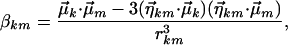
We used an empirical dipole–dipole coupling model to simulate and capture the trends associated with the amide-I band upon denaturation of AK peptide (25, 26). It was assumed that the amide-I manifold of states can be separated from all other vibrational modes. The coupling modifies the nearly degenerate amide-I modes and contributes to the off-diagonal terms of an exciton Hamiltonian matrix in the basis of these modes. These matrix elements can be approximated by the transition dipole-transitiondipole term, βkm:
 |
[1] |
where μk is the effective transition dipole of the kth amide-I mode, η is the unit vector connecting the dipoles, and r is the distance between the dipoles (26). The empirical transition dipole moment has a magnitude of 0.305 D and is located 0.868Å from the carbonyl carbon along the CO bond, directed 20° from the CO bond toward O → N (27). The application of this empirical model must be cautioned because the nearest neighbor interaction may not be properly represented (28).
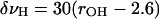
The diagonal matrix elements of the Hamiltonian are sensitive to the amide-I frequency shifts caused by coupling to other modes and to solvent. The contribution to the amide-I frequency fluctuations from H-bonding interactions between the peptide CO and H-bond donors were considered explicitly. Additional amide-I frequency shifts dictated by the fluctuations in geometry were neglected in our calculations. Frequency shifts due to H-bonding interaction were described in terms of geometrical considerations of the solvent molecules or internal atoms which are suitably located to H-bond with CO (16, 29). We define an H-bond as existing when the distance between the hydrogen of a donor and the oxygen of the peptide unit is less than the H-bond cutoff distance (2.6 Å) and makes favorable angles (CO···H and O···HX >90°). When these constraints are satisfied, the diagonal shift in frequency δνH due to H-bonding is given in cm-1 as:
 |
[2] |
where rOH is the CO···HX distance in Å (16, 29–31). When more than one hydrogen atom satisfied the above criteria, the shift was considered to be additive. For specific H-bonding to carbonyls, the amide-I shifts and the additive property are in quantitative agreement with ab initio calculations for structures near the equilibrium H-bonding distances (32–34).
For each configuration, the Hamiltonian was constructed and diagonalized to obtain the excitonic frequencies and intensities. In the calculation of the amide-I spectrum, a separation of time scales between homogeneous and inhomogeneous contributions is assumed. A typical (30) homogeneous dephasing time (T2) of 0.8 ps was used. The ensemble averaging of the frequency spectrum over all configurations obtained from the simulation naturally models the static inhomogeneous contribution to the spectrum and the dephasing describes the motional narrowing in an ad hoc manner. This analysis was carried out at 42 different temperatures. The unperturbed frequency of an amide-I oscillator was chosen to be 1,659 cm-1. For the simulations of the spectra of isotopomers, the zero-order frequencies of labeled carbonyls were shifted by -45 cm-1. The choice of zero-order frequency for this study is not critical because the interest is in the band shape and the changes in the amide-I band with respect to temperature and solvation.
Results and Discussion
Structural Characterization of the Ensembles. To characterize the structural diversity of the different canonical (constant N,V,T) ensembles, we find convenient to generate new ensembles for configurations showing different fraction of helical content (h), for all h = 0–1.0, at 0.1 intervals. The helical content of the AK peptide is calculated according to the Lifson–Roig definition, which requires three consecutive residues to be helical (35). A residue is considered to be helical when the (φ, Ψ) angle lies in the α-helical region of the Ramachandran map, (φ, Ψ) = (-65 ± 35, -37 ± 30). These ensembles can be viewed as a basis set of “pure” states containing only configurations characterized by one order parameter (the fraction of helical content of configurations in the ensemble, h). We call these h-ensembles. At low T, the canonical ensemble will be dominated by high h content, and minor contribution from other configurations, whereas at the transition T (T1/2), the canonical ensemble will have configurations from all h-ensembles.
Conformational Variability and Mobility of Segments. To characterize the dominant structures in the nonhelical (random coil) state, we examined the (φ, Ψ) map for conformations with no helical content (h = 0). In this h-ensemble, the sampling of polyproline-like (PPII) is favored over any other structures. The extended segments of amino acids forming PPII are not as prevalent as observed in (Ala)n peptides (36). Individual residues may also sample the α-helical region, but do not form ordered structures. Based on H-bonding analysis, the 310 helix is populated ≈5% and the contribution from π helix is also minimal in this ensemble. The (φ, Ψ) distribution of segments AK1, AK2, and AK3 exhibited a similar temperature profile. A narrow homogeneous conformational population corresponding to α-helical is found at low T. The N terminus segment, AK1, sampled the PPII region at low T. For AK4, even though primarily a broad α-helical region is populated at lower T, significant populations of PPII and β conformations are also found. As T increases, all segments sample conformational regions belonging to PPII and β structures with higher probability.
End-to-End Distance Distribution. We relate end-to-end distance (d) of the AK peptide to the equilibrium conformations of peptide structures and their distributions that can be detected with Forster resonance energy transfer measurements at the single-molecule level (37–39). Each value of coordinate d corresponds to a large number of configurations and the distribution of which depend on the free-energy landscape explored by the peptide. Fig. 1A shows the end-to-end distance distributions for ensembles at various temperatures. At low T, the distribution has a sharp peak at ≈30 Å, which is consistent with α-helical conformations. At higher T, there are at least two distributions; one near 30 Å, and a broad distribution covering a range of 5–45 Å. Fig. 1B shows the end-to-end distance for h-ensembles characterized by h = 1, 0.5, and 0. The peak near 30 Å clearly represents α-helical structures (h = 1), whereas the broad distribution covering a range of 5–45 Å, and an average distance of 23 Å, characterizes the random coil (h = 0). The relative height of the distribution near 30 Å can be used to measure the content of α-helical configurations in the ensemble. Fig. 1 C and D show histograms of the contribution of various h states to the end-to-end distance distributions at T1/2 (defined by average fractional helical content of 0.5) and at high T. At T1/2, the d distribution is dominated by states with h = 0.5, but there are contribution from other states. At high T, the distribution is dominated by h = 0 states.
Fig. 1.

Nature of structural ensembles that contribute to the observed changes in end-to-end distance (d) distribution during thermal denaturation. (A) the d distribution of the AK peptide at three critical Ts. (B) Characterization of typical end-to-end distributions from structural ensembles (at all T) that are completely random coil (h = 1), half-helical (h = 0.5), and fully helical (h = 0). (C and D) The bar graphs show the helical content of structural ensembles that contribute to the d distribution at T1/2 (C) and high T (D).
Backbone H-Bonding. The main contribution to internal H-bonding arises from i to i + 4 backbone-backbone H-bonding between CO and NH that ensures that residue i + 2 forms a helical turn. Fig. 2 A and B show the CO···HN distance and the relevant angles (∠CO···H and ∠O···HN) of the internal carbonyl H-bonding. For clarity, only the distributions from fully helical (h = 1) and nonhelical (h = 0) h-ensembles are plotted. The helical peptide forms a narrow distribution corresponding i to i + 4 backbone H-bonding. The peak of the distribution is at 2.08 Å and a distance of 2.6 Å encompasses the entire distribution. For random coils, the distribution is very wide and centered at 8 Å. The angular distribution shows a sharp profile for helical structures with the average angles of 153° and 161° for ∠CO···H and ∠O···HN, respectively. In random coils (h = 0), these angles approach an average value of 102°. The geometry of internal H-bonding of the fully helical AK peptide are in quantitative agreement with those found in high-resolution protein crystal structures (40).
Fig. 2.

Geometrical characterization of internal and external carbonyl hydrogen bonding for helical (red) and nonhelical (blue) conformations. For the internal H-bond, the CO···HN distance (A) and the angles (B), ∠CO···H (solid) and ∠O···HN (dashed), are plotted. For external H-bond, the radial distribution function, gO···H(r), for CO···H2O is given for residues 7 (C) and 19 (D). The external H-bonding angles (E), ∠CO···H (solid) and ∠O···HO (dashed) are also plotted for residue 7.
The nature and behavior of external H-bonding (carbonyl H-bonding to water) were different depending on the position, temperature and helicity of AK peptide. For the solvent H-bond, CO···H2O, the radial distribution function, gO···H(r), and angles, ∠CO···H and ∠O···HO were calculated for each residue. Fig. 2 C and D show only the gO···H(r) for two representative residues; one from the middle segment (residue 7), and the other from the C terminus (residue 19). In helices, the gO···H(r) of residue 7 peaks at 1.9 Å with a well defined first-solvent shell given by a radial distance of 2.6 Å. The ∠CO···H angle is 118° (Fig. 2E); smaller than the angle obtained for internal H-bonding. The difference is the result of a competition between the carbonyl forming H-bonding to the backbone and solvent. The ∠O···HO angle is similar to the one found for internal H-bonding but has a much wider distribution. In random coils (h = 0), the peak height of gO···H(r) increases indicating greater solvation. However, the residue 19 from the C terminus shows an opposite trend. For helices, the gO···H(r) peak is sharp and high, indicating well defined solvation with increased coordination of water molecules. The decrease in peak intensity of gO···H(r) in random coils indicates that C terminus residues are not solvated to the same extent as in helices. Mean values for angles, ∠CO···H and ∠O···HO are 128° and 161°, respectively. The distribution is similar to the random coil angular distribution found for residue 7. Regardless of the helical content of the conformers, the peptide carbonyls from the C terminus segment are solvated to a greater degree than those from the mid segment. The mean H-bonding distance in solvent H-bonds is shorter than in helical H-bonds but the ∠CO···H angle is more linear with a sharper distribution in helical H-bonds.
The Effect of Structural Inhomogeneities in the Amide-I Band
Dependence of Coupling on Conformational Variability. The conformational heterogeneities of the random coil (h = 0) ensemble give rise to different coupling strengths between amide-I modes. To illustrate the dependence of coupling on conformations, the distribution of coupling strength arising from interaction between nearby amide units is shown when the peptide is fully helical versus completely nonhelical. In Fig. 3, the distributions of coupling strengths between i and i + 1, i and i + 2, i and i + 3, and i and i + 4 are plotted for the same two scenarios (h = 0 and h = 1). For the h = 1 ensemble, the coupling is uniform across the helix and has narrow distributions. The strongest coupling (≈9 cm-1) arises from the neighboring amide units and is positive. The strongest negative coupling (approximately -6 cm-1) arises from interaction between i and i + 3 amide units. The helical H-bond to HN of (i + 4)th residue aligns the CO of (i + 3)th residue, which forms the peptide bond with that HN, for this favorable interaction. The empirical dipole–dipole couplings compare well with measured coupling constants in a similar helical peptide where values of 9.5 cm-1 and -5.5 cm-1 were reported for the i, i + 1 and i, i + 3 interactions, respectively (41). For the h = 0 ensemble, the translational symmetry (uniformity) of the coupling along the helical backbone is lost. The distribution becomes broader and has zero mean. There are also significant coupling interactions at random along the helix and also between amide-I units having large separations in the sequence.
Fig. 3.

The distribution of coupling between important pairs of nearby amide-I modes for fully helical (solid line) and completely nonhelical (dash line) ensembles of AK peptide. The distribution of coupling strengths (in cm-1) is plotted for interaction between the following pairs; i and i + 1(A), i and i + 2 (B), i and i + 3 (C), and i and i + 4 (D).
Frequency Shifts Due to Carbonyl Hydrogen Bonding. The H-bonding of backbone carbonyl of peptides causes the amide-I band to shift toward lower frequencies. A simple linear model (Eq. 2) based on the geometry of H-bond is used to calculate the resulting shift in the amide-I band toward lower frequency (16, 29–31). Fig. 4A shows the total amide-I frequency shift, from both internal and external H-bonding, for the labeled segments of AK peptide as a function of T. For all segments, the magnitude of the shift decreases with increasing T. The segments AK1, AK2, and AK3, show a similar profile with T where the amide-I frequency shifts by ≈28.3 cm-1 at low T and decreases to 21.7 cm-1 as T increases. The C terminus segment show a larger shift compared with other segments at all T: 30.5 cm-1 at low T and 23.6 cm-1 at high T.
Fig. 4.

The dependence of amide-I frequency on the internal and external hydrogen bonding as a function of T. The plot shows that the magnitude of amide-I frequency shifts toward lower frequency due to H-bonding of carbonyls from different segments of the AK peptide. The total frequency shift (A) and the contribution to the shift just due to the solvent H-bonding (B) are shown.
The contribution from external H-bonding to the amide-I band is also examined (Fig. 4B). Segments AK1, AK2, and AK3 show a trend where the frequency shift decreases until approximately T1/2, then increases with T. The overall contribution to amide-I frequency shift due to H-bonding to solvent is on the order of 12–15 cm-1. The frequency shift due to H-bonding of the C terminus segment continuously decreases with increasing T. The magnitude of the shift is also higher by 10 cm-1 compared with other segments. The large shift is correlated to the increase in number of water molecules coordinated to the C terminus carbonyls at lower T. There is a preference for forming two solvent H-bonds at the C terminus when the peptide is helical.
Simulation of the Amide-I Band
Solvated Helix Versus Buried Helix. An important question regarding the amide-I spectrum of a solvated helix is whether the side chains provide shielding across the entire helix such that amide-I frequency shift arises solely from the internal H-bonding. There is experimental evidence for the solvation of the exposed backbone being responsible for the amide-I shift toward lower frequencies, which does not occur for buried helices (4, 42, 43). Molecular dynamics simulations also showed evidence of hydration of helices (12, 44, 45). The direct effect of solvation on the amide-I band is that it reduces the force constant of the individual amide oscillators. The solvent also indirectly affects the amide-I band by changing conformational preferences, which in turn results in different coupling strengths. We find that the calculated amide-I band of the solvated AK peptide is positioned near 1,630 cm-1 at low T. By neglecting carbonyl H-bonds to water in the calculation, we carried out a similar calculation for desolvated/buried AK peptide. The solvated band is shifted by ≈12 cm-1 toward the lower frequency compared with the buried one at room temperature (Fig. 7A, which is published as supporting information on the PNAS web site). The major contribution to the observed frequency shift of the amide-I band arises due to the strong tendency for carbonyls to form H-bonds with water even though they are internally H-bonded. At low T, the solvent H-bonding is present with 50–70% probability. The overall change in solvation upon going from low to high T is not drastic and results in an increase of only ≈20%. The H-bonding to solvent at low T is not uniform along the helix. Significant shielding due to Lys side chains occurs at Ala residues 1, 6, 11, and 16. A microscopic picture of water shielding in helical peptides, including the role of Arg and Lys in shielding the backbone carbonyls, have been described (12, 46). The coordination number of water molecules is lower at these positions (Fig. 7B). The effect of shielding on the amide-I band is partially masked by a stronger helical H-bond at these positions.
Thermal Denaturation of Helix. In the experiments by Decatur (14), the amide-I band showed a maximum at 1,634 cm-1, which is indicative of α-helices. With increasing T, the intensity of this band decreased and the band maximum shifted to 1,646 cm-1 at 55°C, which is indicative of random coils. First, we evaluate how accurate is the association of amide-I band to existence of helical and random configurations from measurements at low and high T, respectively. Fig. 5A shows the calculated amide-I band from helical (h = 1) and random coil (h = 0) h-ensemble configurations. The helical ensemble give rise to a narrower band at lower frequency compared with the random coil ensemble. Fig. 5B provides the distributions of h-ensembles at low T, T1/2, and high T.
Fig. 5.

The behavior and nature of amide-I band on thermal denaturation. (A) The amide-I band from completely helical and nonhelical ensembles. (B) The distribution of helical states between the above limits is shown at three different T. (C) The amide-I spectra at 21 different T. (D) The loss in intensity at 1,629 cm-1 (maximum peak at low T) and the helical content are plotted as function of T.
The calculated IR spectra are plotted in Fig. 5C for 21 different temperatures, ranging from 273 to 551K. At low T, the amide-I band peaks at 1,629 cm-1. As T increases, the band shifts to 1,641 cm-1 and it broadens. These temperature-dependent changes are consistent with the measured amide-I spectra of the AK peptide (14). The fractional helical content is plotted in Fig. 5D as a function of T alongside the loss in intensity at 1,629 cm-1 (the peak maximum at the lowest T). At the lowest T, the helical content is ≈90%. It decays to 20% at very high T. The Lifson–Roig helical content profile describes a helix–coil transition that is not strongly cooperative with a T1/2 of ≈450K. Interestingly, the helix–coil transition from the amide-I band intensities calculated from the same set of trajectories describes a more cooperative transition, and the half-height of the peak intensity occurs at much lower T (380K). The discrepancy in the helical content versus T profiles is due to the marked sensitivity of the IR coupling to geometry. In the Lifson–Roig approach, we allowed for (φ, Ψ) variations of ≈30° to define helical configurations that may result in large changes in amide-I couplings.
The shift of amide-I band toward the higher frequency with increasing T is caused by the breaking of helical H-bonds. One might expect that the effect of diminishing helical H-bonds would be fully compensated by solvent H-bonds upon denaturation, but this is not the case. Even though there is an increase in carbonyl H-bonding to water in the random coil, that increase does not compensate the loss of helical H-bonds. Therefore, the overall frequency shift due to hydrogen bonding decreases with increasing T and contributes to the observed shift toward high frequency of amide-I band. The changes in the coupling between amide-I oscillators contribute significantly to the broadening of the band. For a fully helical peptide, the coupling interactions are local and uniform along the helix, resulting in high oscillator strength for lower energy states. At high T, the translational symmetry of the coupling along the helix is broken (Fig. 3). The amide-I mode coupling interactions become random and both local and nonlocal in nature. This action spreads the oscillator strength over a wide range of states and leads to broadening.
Interpretation of Isotope-Labeled IR. The REMD simulations also describe the properties of the vibrational spectra of helices on a segment-by-segment basis, allowing a microscopic interpretation of experiments (14) on isotopically substituted helices in terms of local helical content. For the AK peptide, we predict quite different spectral properties for each of the labeled AAAA segments in agreement with what is observed experimentally. The calculated IR spectra are shown in Fig. 6 for the four isotopomers, AK1, AK2, AK3, and AK4. At low T, the AK2 and AK3 have a similar amide-I spectrum with a well defined 12CO peak and a resolved but weaker 13CO band downshifted from the main band. The effect of labeling is prominent for AK2 and AK3 because the labeling interrupts the uniform excitonic coupling of near resonance oscillators. At high T, the amide-I band is dominated by the inhomogeneous distribution of frequencies from the nonuniform coupling, resulting in broad overlapping 12CO and 13CCO bands. For the AK1, the 13CO amide-I peak is not well resolved as for AK2 and AK3. The AK4 has just a broad shoulder for the 13CO band. The observed differences in the 13CO band are sensitive indicators of the coupling and frequency differences between the local segments.
Fig. 6.

The calculated amide-I spectra for the thermal denaturation of the isotopomers of the AK peptide. (A) AK1. (B) AK2. (C) AK4. The spectrum for AK3 is similar to that of AK2. The arrowed lines mark the direction of spectrum from low to high T, ranging from 275 to 541K. (D) Difference spectra (labeled–unlabeled) for two cases; labeling residue 11, which is partially shielded from the solvent (solid line), and residue 12, which is not shielded from the solvent (dashed line) shown at the lowest T.
We attribute the differences in intensities of the 13CO band to the differences in helical content of the local segments (15). The Lifson–Roig helical content profiles of individual segments (Fig. 8, which is published as supporting information on the PNAS web site) predict that the N terminus and the middle segments contribute equally to the overall helical content (21%), whereas the C terminus segment, AK4, has the lowest (7%). The observed 13CO peak intensities (figure 6 in ref. 14) fit that profile. A quantitative assertion of this relationship is obtained by comparing the calculated peak intensities of labeled 13CO band (Fig. 6) and the segmental helical content calculated from the same atomic trajectories (Fig. 8A). It validates the correlation between the large local helical content and the high intensity 13CO peaks of AK2 and AK3. The C terminus segment, AK4, has the lowest helical content and showed the least amplitude for the 13CO band. A similar relationship can be stated for the unlabeled segment of the peptide (Fig. 8B) that can be profiled by monitoring the 12CO band peak. AK2 and AK3 exhibit 12CO amide-I bands with low-intensity peaks and can also be rationalized based on local helical content. The terminal segments possess lower helical content compared to the middle segments. Consequently, when the middle segments are labeled, the helical content from the rest of the peptide is lower (69%), compared with the case when terminal segments are labeled (76%). The labeling of four consecutive Ala does not expose the effect of partial shielding from water due to Lys side chains observed at specific Ala residues in our simulations (Fig. 7B). We predict that the manifestation of the shielding effect can be better deduced from isotope IR by labeling a single Ala residue at shielded and unshielded positions. We calculated the amide-I band for labeling residue 11 (shielded) and 12 (unshielded), one at a time. In Fig. 6D, the difference spectra (labeled–unlabeled) show a clear distinction between the shielded and unshielded case. Even though the difference is subtle, it is consistent with other shielded and nonshielded locations.
Conclusions
The main objective of the simulations and analysis presented here is to offer a quantitative basis for the vibrational spectra of different helical conformations. In particular, we aimed to compare the calculation with temperature-dependent IR experiments that probe the amide-I region. Previous theoretical studies (19, 47, 48) of vibrational spectra have not incorporated the structural inhomogeneities that contribute to the line shapes and their dependence on temperature, solvation, and conformational distribution. The REMD simulations capture the nature and behavior of conformational variability and carbonyl H-bonding. The definition of h-ensembles permits the evaluation of end-to-end distance profiles and vibrational frequencies and inter-mode coupling in term of states characterized by their helical content. This analysis was used to provide insight into the effect on the amide-I band of solvation and thermal denaturation. The observations from isotope IR aimed at the characterization of the unfolded state along the chain can now be interpreted with a solid structural basis.
The multidimensional IR techniques can provide measurements of structural inhomogeneities (16, 17). Therefore, knowledge of the coupling and hydrogen bonding distributions of folded and unfolded states will assist in the modeling of 2D IR spectra of partially unfolded distributions of helices. We have also illustrated how the structural ensembles obtained from REMD provide predictions of distributions of states that could be measured in single molecule experiments on the folding of helices.
Supplementary Material
Acknowledgments
We thank H. Nymeyer for assistance with the REMD simulations and S. Decatur and R. Schweitzer-Stenner for discussions. This work was supported by funds from the Laboratory-Directed Research and Development Program at Los Alamos National Laboratory and by National Institutes of Health Grants GM12592 and RR01348 (to R.M.H.).
Abbreviations: T, temperatures; REMD, replica-exchange molecular dynamics; PPII, polyproline-like.
References
- 1.Marqusee, S., Robbins, V. H. & Baldwin, R. L. (1989) Proc. Natl. Acad. Sci. USA 86, 5286-5290. [DOI] [PMC free article] [PubMed] [Google Scholar]
- 2.Vila, J., Williams, R. L., Grant, J. A., Wojcik, J. & Scheraga, H. A. (1992) Proc. Natl. Acad. Sci. USA 89, 7821-7825. [DOI] [PMC free article] [PubMed] [Google Scholar]
- 3.Martinez, G. & Millhauser, G. (1995) J. Struct. Biol. 114, 23-27. [DOI] [PubMed] [Google Scholar]
- 4.Dyer, R. B., Gai, F. & Woodruff, W. H. (1998) Acc. Chem. Res. 31, 709-716. [Google Scholar]
- 5.Williams, S., Causgrove, T. P., Gilmanshin, R., Fang, K. S., Callender, R. H., Woodruff, W. H. & Dyer, R. B. (1996) Biochemistry 35, 691-697. [DOI] [PubMed] [Google Scholar]
- 6.Decatur, S. M. & Antonic, J. (1999) J. Am. Chem. Soc. 121, 11914-11915. [Google Scholar]
- 7.Huang, C. Y., Getahun, Z., Wang, T., Degrado, W. F. & Gai, F. (2001) J. Am. Chem. Soc. 123, 12111-12112. [DOI] [PubMed] [Google Scholar]
- 8.Lednev, I. K., Karnoup, A. S., Sparrow, M. C. & Asher, S. A. (1999) J. Am. Chem. Soc. 121, 8074-8086. [DOI] [PubMed] [Google Scholar]
- 9.Sugita, Y. & Okamoto, Y. (1999) Chem. Phys. Lett. 314, 141-151. [Google Scholar]
- 10.Sanbonmatsu, K. Y. & Garcia, A. E. (2002) Proteins 46, 225-234. [DOI] [PubMed] [Google Scholar]
- 11.Garcia, A. E. & Sanbonmatsu, K. Y. (2001) Proteins 42, 345-354. [DOI] [PubMed] [Google Scholar]
- 12.Garcia, A. E. & Sanbonmatsu, K. Y. (2002) Proc. Natl. Acad. Sci. USA 99, 2782-2787. [DOI] [PMC free article] [PubMed] [Google Scholar]
- 13.Gnanakaran, S. & Garcia, A. E. (2003) Biophys. J. 84, 1548-1562. [DOI] [PMC free article] [PubMed] [Google Scholar]
- 14.Decatur, S. M. (2000) Biopolymers 54, 180-185. [DOI] [PubMed] [Google Scholar]
- 15.Venyaminov, S. Y., Hedstrom, J. F. & Prendergast, F. G. (2001) Proteins 45, 81-89. [DOI] [PubMed] [Google Scholar]
- 16.Gnanakaran, S. & Hochstrasser, R. M. (2001) J. Am. Chem. Soc. 123, 12886-12898. [DOI] [PubMed] [Google Scholar]
- 17.Zanni, M. T. & Hochstrasser, R. M. (2001) Curr. Opin. Struct. Biol. 11, 516-522. [DOI] [PubMed] [Google Scholar]
- 18.Gnanakaran, S., Nymeyer, H., Portman, J., Sanbonmatsu, K. Y. & Garcia, A. E. (2003) Curr. Opin. Struct. Biol. 13, 168-174. [DOI] [PubMed] [Google Scholar]
- 19.Silva, R. A. G. D., Kubelka, J., Bour, P., Decatur, S. M. & Keiderling, T. A. (2000) Proc. Natl. Acad. Sci. USA 97, 8318-8323. [DOI] [PMC free article] [PubMed] [Google Scholar]
- 20.Darden, T., York, D. & Pedersen, L. (1993) J. Chem. Phys. 98, 10089-10092. [Google Scholar]
- 21.Ryckaert, J.-P., Ciccotti, G. & Berendsen, H. J. C. (1977) J. Comput. Phys. 23, 327-341. [Google Scholar]
- 22.Hoover, W. G. (1985) Phys. Rev. A. 31, 1695-1697. [DOI] [PubMed] [Google Scholar]
- 23.Jorgensen, W. L., Chandrasekhar, J., Madura, J. D., Impey, R. W. & Klein, M. L. (1983) J. Chem. Phys. 79, 926-935. [Google Scholar]
- 24.Gnanakaran, S. & Garcia, A. E. (2003) J. Phys. Chem. B. 107, 12555-12557. [Google Scholar]
- 25.Torii, H. & Tasumi, M. (1992) J. Chem. Phys. 96, 3379-3387. [Google Scholar]
- 26.Krimm, S. & Bandekar, J. (1986) Adv. Protein Chem. 38, 181-364. [DOI] [PubMed] [Google Scholar]
- 27.Rabolt, J., Moore, W. & Krimm, S. (1977) Macromolecules 10, 1065-1074. [DOI] [PubMed] [Google Scholar]
- 28.Moran, A. & Mukamel, S. (2004) Proc. Natl. Acad. Sci. USA 101, 506-510. [DOI] [PMC free article] [PubMed] [Google Scholar]
- 29.Woutersen, S. & Hamm, P. (2001) J. Chem. Phys. 115, 7737-7743. [Google Scholar]
- 30.Hamm, P., Lim, M. H. & Hochstrasser, R. M. (1998) J. Phys. Chem. B. 102, 6123-6138. [Google Scholar]
- 31.Scheurer, C., Piryatinski, A. & Mukamel, S. (2001) J. Am. Chem. Soc. 123, 3114-3124. [DOI] [PubMed] [Google Scholar]
- 32.Ham, S., Kim, J. H., Lee, H. & Cho, M. H. (2003) J. Chem. Phys. 118, 3491-3498. [Google Scholar]
- 33.Torii, H., Tatsumi, T. & Tasumi, M. (1998) J. Raman Spectrosc. 29, 537-546. [Google Scholar]
- 34.Torii, H., Tatsumi, T., Kanazawa, T. & Tasumi, M. (1998) J. Phys. Chem. B 102, 309-314. [Google Scholar]
- 35.Lifson, S. & Roig, A. (1961) J. Chem. Phys. 34, 1963-1974. [Google Scholar]
- 36.Garcia, A. E. (2004) Polymer 45, 669-676. [Google Scholar]
- 37.Lipman, E. A., Schuler, B., Bakajin, O. & Eaton, W. A. (2003) Science 301, 1233-1235. [DOI] [PubMed] [Google Scholar]
- 38.Schuler, B., Lipman, E. A. & Eaton, W. A. (2002) Nature 419, 743-747. [DOI] [PubMed] [Google Scholar]
- 39.Talaga, D. S., Lau, W. L., Roder, H., Tang, J. Y., Jia, Y. W., Degrado, W. F. & Hochstrasser, R. M. (2000) Proc. Natl. Acad. Sci. USA 97, 13021-13026. [DOI] [PMC free article] [PubMed] [Google Scholar]
- 40.Kortemme, T., Morozov, A. V. & Baker, D. (2003) J. Mol. Biol. 326, 1239-1259. [DOI] [PubMed] [Google Scholar]
- 41.Fang, C., Wang, J., Charnley, A., Barber-Armstrong, W., Smith, A., Decatur, S. & Hochstrasser, R. (2003) Chem. Phys. Lett. 382, 586-592. [Google Scholar]
- 42.Heimburg, T., Schunemann, J., Weber, K. & Geisler, N. (1999) Biochemistry 38, 12727-12734. [DOI] [PubMed] [Google Scholar]
- 43.Manas, E. S., Getahun, Z., Wright, W. W., Degrado, W. F. & Vanderkooi, J. M. (2000) J. Am. Chem. Soc. 122, 9883-9890. [Google Scholar]
- 44.Garcia, A. E., Hummer, G. & Soumpasis, D. M. (1997) Proteins 27, 471-480. [PubMed] [Google Scholar]
- 45.Walsh, S. T. R., Cheng, R. P., Wright, W. W., Alonso, D. O. V., Daggett, V., Vanderkooi, J. M. & Degrado, W. F. (2003) Protein Sci. 12, 520-531. [DOI] [PMC free article] [PubMed] [Google Scholar]
- 46.Ghosh, T., Garde, S. & Garcia, A. (2003) Biophys. J. 85, 3187-3193. [DOI] [PMC free article] [PubMed] [Google Scholar]
- 47.Bour, P., Kubelka, J. & Keiderling, T. (2002) Biopolymers 65, 45-59. [DOI] [PubMed] [Google Scholar]
- 48.Lee, S. H. & Krimm, S. (1998) Biopolymers 46, 283-317. [Google Scholar]
Associated Data
This section collects any data citations, data availability statements, or supplementary materials included in this article.