xiNET: Cross-link Network Maps With Residue Resolution

Abstract

xiNET is a visualization tool for exploring cross-linking/mass spectrometry results. The interactive maps of the cross-link network that it generates are a type of node-link diagram. In these maps xiNET displays: (1) residue resolution positional information including linkage sites and linked peptides; (2) all types of cross-linking reaction product; (3) ambiguous results; and, (4) additional sequence information such as domains. xiNET runs in a browser and exports vector graphics which can be edited in common drawing packages to create publication quality figures. Availability: xiNET is open source, released under the Apache version 2 license. Results can be viewed by uploading data to http://crosslinkviewer.org/ or by downloading the software from http://github.com/colin-combe/crosslink-viewer and running it locally.

Cross-linking/mass spectrometry (CLMS)¹ has revealed protein–protein interactions in large multiprotein complexes (1), small networks (2), and complex mixtures (3). When cross-links are observed they define a pair of residues that are close in space and in this way reveal not just the identity of interacting proteins but also pinpoint interacting regions or domains and their orientation. A common feature of CLMS studies is identifying many individual cross-links that cumulatively support the existence of domain-level features. Making this connection between the network of residue distance constraints and domain-level features is difficult if looking at a large table of CLMS data. A visual analysis that highlights clusters of cross-links within the protein sequence helps greatly. As we shall see (“Node Layouts”), not all visualizations of the network will allow this.

There are two types of network visualization: node-link diagrams and adjacency matrices. Each has its own advantages and disadvantages. Node-link diagrams preserve the local detail of the network but do not scale well. Adjacency matrices avoid the edge crossings that make large node-link diagrams unreadable, but make it difficult to understand the relationships between nodes that are not directly connected (4). Seebacher et al. (5) show CLMS data visualized as an adjacency matrix. Here, we focus on visualizing CLMS data as a node-link diagram and present xiNET, a network visualization tool designed specifically for use with CLMS data.

Comparable Software

In 2010, Gehlenborg et al. (6) provided a review of the then state-of-the-art visualization tools for “omics” data in systems biology. They begin by noting that all these tools are dominated by the same primary visual metaphor: graphs displayed as node-link diagrams. Their review is, essentially, a review of the use of node-link diagrams in biology. They continue by identifying two broad, partly overlapping, categories of visualization tools–pathway tools and network tools. Pathway tools display a graph representing changes in state over time; network tools display graphs that do not (necessarily) include state change information.

CLMS can provide data on conformational changes within proteins, hence state change is one aspect of this data. However, we will narrow our focus here by concentrating on network tools that do not set out to represent state change. Gehlenborg et al. present a second categorization of network tools corresponding to the three main types of high throughput experiment. The categories are: tools for investigating protein-protein interactions, tools for investigating gene expression profiles, and tools for investigating metabolic profiles. They list 27 software packages specifically intended for investigating protein-protein interaction networks—a list that has continued to grow since 2010. Of these 27, they recommend two—CytoScape (7) and Cerebral (8).

CytoScape is perhaps the most popular network visualization tool in biology. The CytoScape software provides a plugin architecture that allows extension and customization. For example, a new node layout algorithm could be added. Cerebral is a CytoScape plugin that uses additional annotation information, particularly subcellular location, to guide the layout of the nodes. Its aim is to produce interaction network diagrams that more closely resemble “traditional” signaling pathway/system diagrams, with extracellular proteins and membrane receptors at the top of the page, moving down through adapter proteins in the cytoplasm, with nuclear proteins and pathway-regulated genes at the bottom.

In biology, node-link diagrams typically use the nodes to represent entire molecules (4). Much of the discussion of protein–protein interaction tools in Gehlenborg et al.'s 2010 review focuses on arranging the nodes that represent molecules according to the higher order structures (complexes and groups of complexes) that they make up. Related to this are approaches that display a hierarchical graph and in which nodes representing individual molecules can be collapsed into a single meta-node representing a higher order grouping. An example of such software is Visant (9).

When discussing future directions for the network visualization of omics data, Gehlenborg et al. highlight improved navigation methods for large networks, a trend toward web-based tools, and the need for standardization of data formats. PSI-MI (10) is highlighted with regards the standardization of interaction data. However, nowhere in their review is there a discussion of breaking the molecule-level nodes down into smaller parts.

An alternative to representing whole bio-molecules as nodes is to use distinct nodes to represent distinct residues, and there are tools that do this. It is often seen in tools for analyzing residue interaction networks (RINs) derived from protein data bank (PDB) (11) models. RINalyzer (12) is an example of such a tool. It is used to analyze conformational changes (for example, as a result of mutations) or when looking at long-range residue relationships (the path of information through a structure, e.g. allosteric effects). RINalyzer uses the three-dimensional PDB model to guide the layout of the nodes in the two-dimensional network diagram. Although crystal structures or models are interesting in the context of CLMS data, for most proteins we do not hold such data and in fact about one-third of sequence space is unstructured. RINalyzer cannot currently import other types of data such as cross-links. Again, RINalyzer is implemented as a CytoScape plugin. Broadly comparable to RINalyzer is RING (13), it also generates a RIN from a PDB file and visualizes this via a CytoScape plugin. RING lacks RINalyzer's ability to use the PDB model to guide the node layout in CytoScape. A third RIN tool we find worthy of mention is ResMap (14). Not a CytoScape plugin, but a stand-alone application, ResMap displays the interacting residues along an axis representing the protein sequences (or part thereof). However, ResMap is limited by only allowing the visualization of interactions between any two subunits of the PDB model (that is, it can only display two axes).

These RIN tools have the most in common with our needs for visualizing CLMS data, as it is a network of interacting residues that CLMS data provides. Setting aside practical questions about importing CLMS data into existing RIN tools, these tools still do not meet our needs for visualizing such data. To understand why, it is necessary to look at the question of node layout in more detail.

Node Layouts

We have noted that a typical biological use case for CLMS data is drawing conclusions about domain-level features from the many individual identified cross-links. The residue distance constraints from a CLMS experiment form an undirected graph and there are many two-dimensional network visualization tools available that could be used to display such a graph. However, there are specific requirements for a visualization that allows clusters of linked residues within the protein sequence to be seen, thereby elucidating the location of domain-level features.

This is illustrated in Fig. 1, which shows six node-link representations of the same CLMS data. For simplicity, we use only the inter-protein cross-links from this dataset, omitting self-links (links back to a protein of the same type). The data is taken from Chen et al. (1), who investigated the structure of the RNA polymerase II-TFIIF complex. Essential to their conclusions is CLMS evidence for the locations of dimerization domains between Tfg1 and Tgf2.

Fig. 1.

Six different node-link diagrams of the same CLMS data. The data is from Chen et al. (1), A, is an extract from that paper designed to show how the CLMS evidence supports the location of a dimerization domain between Tfg1 and Tfg2. B–F, show alternative node-link diagrams (of the interprotein links only) produced using D3 (20). B, shows the typical use of node-link diagrams in biology, where nodes represent whole molecules (line width has been used to represent the number of links). C, uses distinct nodes to represent the linked residues, as is typical of RIN tools such as RINalyzer (12). In the absence of other information to guide the layout, C, uses a force directed layout. D, attempts to bring some order to the layout by arranging the nodes around a circle. E, again uses a circular layout but this time the placement of the nodes on the perimeter is determined by the linked residue's position in the protein sequence. F, shows a HivePlot (16) of the data, in which the categories (axes) represent each of the three proteins and the distance along the axis is determined by residue position in the sequence. A, E and F succeed in making an association between the individual cross-links and domain-level features: B, C, and D do not. To make this association it is necessary to use the position of the linked residues within the overall protein sequence to guide the placement of the nodes.

Fig. 1A is a Chen et al paper. Its purpose was to graphically depict this evidence for the location of the domains. It is a type of node-link diagram which represents the protein sequences as numbered bars and cross-links as lines ending at points along these bars. However, there are many other possible ways of arranging the nodes, some of which will achieve an effect similar to Fig. 1A.

Fig. 1B shows the CLMS data for TFIIF in the way most commonly found in biology, with nodes representing whole molecules. Unsurprisingly, it entirely fails to depict the location of the dimerization domains within the protein sequence because the residue-level information is missing. However, there are cross-linking studies that do visualize their results in this way (2, 15). For some purposes visualizing the data at this level of abstraction is appropriate. A specific challenge with regards CLMS data is the presence of two levels of information—linked residues and linked proteins—as either could be the nodes in a graph.

An alternative to representing whole bio-molecules as nodes, is to use distinct nodes to represent distinct residues, as is seen in RINalyzer and RING. Fig. 1C shows our example TFIIF CLMS data in this style. Each linked residue is a separate node, but without a PDB model used to guide the layout of the nodes (as RINalyzer would use). It does not help indicate the location of the dimerization domains in the protein sequences. Part of the reason this approach does not work well is that the residue networks that derive from current cross-link data are much less densely connected than those derived from PDB data.

More generally, Fig. 1C fails because of the arbitrary positioning of the nodes in a meaningless coordinate space (16). In addition to problems scaling, this is another well-known problem with node-link diagrams and the positioning of the nodes greatly affects how the data is perceived (4). The positioning of the nodes in Fig. 1C can be altered such that it will achieve a similar effect to Fig. 1A, informing us about the location of the domains. To do this, the function used to position the nodes must consider the linked residues they represent within the context of the whole protein sequence. To see this, compare Fig. 1D and Fig. 1E. Both order the arrangement of the linked residue nodes around a circle, but only Fig. 1E is informative about the position of the links within the protein sequences. When positioning the nodes, Fig. 1E considers their location within the overall protein sequence, while Fig. 1D does not.

Fig. 1F shows a HivePlot (16) of the TFIIF data. It meets the criteria of using the position of the linked residues within the overall protein sequence when arranging the nodes. Hence, it succeeds in making the connection between the CLMS evidence and the locations of the dimerization domains within the proteins. In a HivePlot, the axes are categories of node; in Fig. 1F these categories represent the three proteins included in the data and the ordering function for the position along each axis is based on the residue position within the sequence. HivePlots work less well when there are more than three categories (that is, more than three axes, or, in our specific case, more than three proteins).

Arranging the linked residues along axes representing the protein sequences, as ResMap does (although ResMap is limited to displaying interactions between two subunits), is the visualization mode we find useful for CLMS data. Fig. 1A, the extract from Chen et al.(1), could be thought of as a HivePlot (constructed as described above), but with the axes moved around and rotated.

Benefits of xiNET

Here, we present xiNET—an automated tool for generating interactive versions of the “numbered bar” style of node-link diagram (seen in Fig. 1A). This numbered bar layout has often been used in CLMS papers, for examples (1, 17, 18, 19). It is not the only approach to visualizing this data that could show how the many cross-links support the location of domain-level features. There are other ways, some of which could, for example, be implemented as CytoScape plugins. However, the numbered bar approach is visually concise, not requiring a distinct glyph for each linked residue node, and allows flexibility about the relative positioning of the axes. These diagrams use this flexibility to emphasize closely connected regions.

By showing the linked residues within the context of the overall protein sequence xiNET addresses an important biological use-case when working with CLMS data. However, xiNET has other features beyond this that will help advance scientific understanding.

xiNET represents ambiguous cross-links. Ambiguity regarding the linkage site can occur if, for example, an identified cross-linked peptide belongs to more than one protein in the search space. Such ambiguous links may contain potentially important structural information yet can be confusing or misleading if not represented clearly.

xiNET also represents and distinguishes all cross-linking product types. In addition to cross-linked peptides, cross-linking reactions generate linker modified peptides and internally linked peptides. All three product types contain structural information. The location of linker-modified peptides (“protein painting”) shows which areas of the protein were solvent accessible. An absence of linker-modified peptides in an area where they would be expected can indicate that the surface was occluded. Internally linked peptides provide further residue distance constraints, however, the structural significance of these links differ from that of cross-linked peptides and so they should be distinguished in the visualization. An internally linked peptide is known to result from an intramolecular cross-link. Most cross-linked peptides in which both peptides come from the same protein could be either intra or intermolecular. However, there is a subset of cross-linked peptides in which the peptides overlap in the protein sequence and these are known to be intermolecular. xiNET also distinguishes these links—self-links that could only be derived from homomultimers.

Another reason for the popularity of the numbered bar representation in CLMS papers is that it allows the links to be shown in the context of other residue-resolution sequence information such as domains. xiNET automatically retrieves such annotations (or they can be specified manually) and incorporates them into the diagram. This further contextual information assists with hypothesis generation.

We noted that the node-link diagrams in which nodes represent whole molecules are also a common network representation of CLMS data, and that this level of abstraction may be appropriate for certain purposes. xiNET allows both these forms to be mixed together: the data can be collapsed to protein level (one node represents the whole protein) or expanded to show the linked residues along a numbered bar. This allows the user to select which parts of the network are shown in more or less detail.

All these preceding features are demonstrated in the Results section. Lastly, xiNET facilitates the communication of CLMS data. It does this by being web based, making it easy to share the interactive figures, and providing vector graphic output that can be used to create publication quality figures. This enhanced communication can itself help advance scientific understanding.

Implementation

xiNET is written in JavaScript and manipulates a scalable vector graphic (SVG) element within a web page. The interactive maps embedded in web pages can be easily shared. The SVG output can be edited in common vector drawing packages, such as Inkscape or Illustrator.

We have used D3.js (20) as a utility library for common visualization needs such as color schemes. The xiNET code has an object-oriented design and the following object types make up the model: Match (representing a matched spectrum); Residue Link (an aggregation of all the matches between a pair of residues); Protein Link (an aggregation of all the residue links between two proteins); and Protein.

Fig. 2 provides an overview of the xiNET workflow. The input data sets for a cross-link map are: cross-link data; protein sequence data; and, optionally, annotation data. Sequence data can be omitted if UniProtKB (21) accession numbers are used as the protein identifiers, in this case protein sequences will be retrieved automatically using a web-service provided by UniProt¹. If UniProtKB accession numbers are used then annotation data will also be retrieved from this web-service and from the SuperFamily (22) Distributed Annotation System (23) server². Once data has been loaded into xiNET the CLMS network can be interactively explored and vector graphics can be exported for use in figures.

Fig. 2.

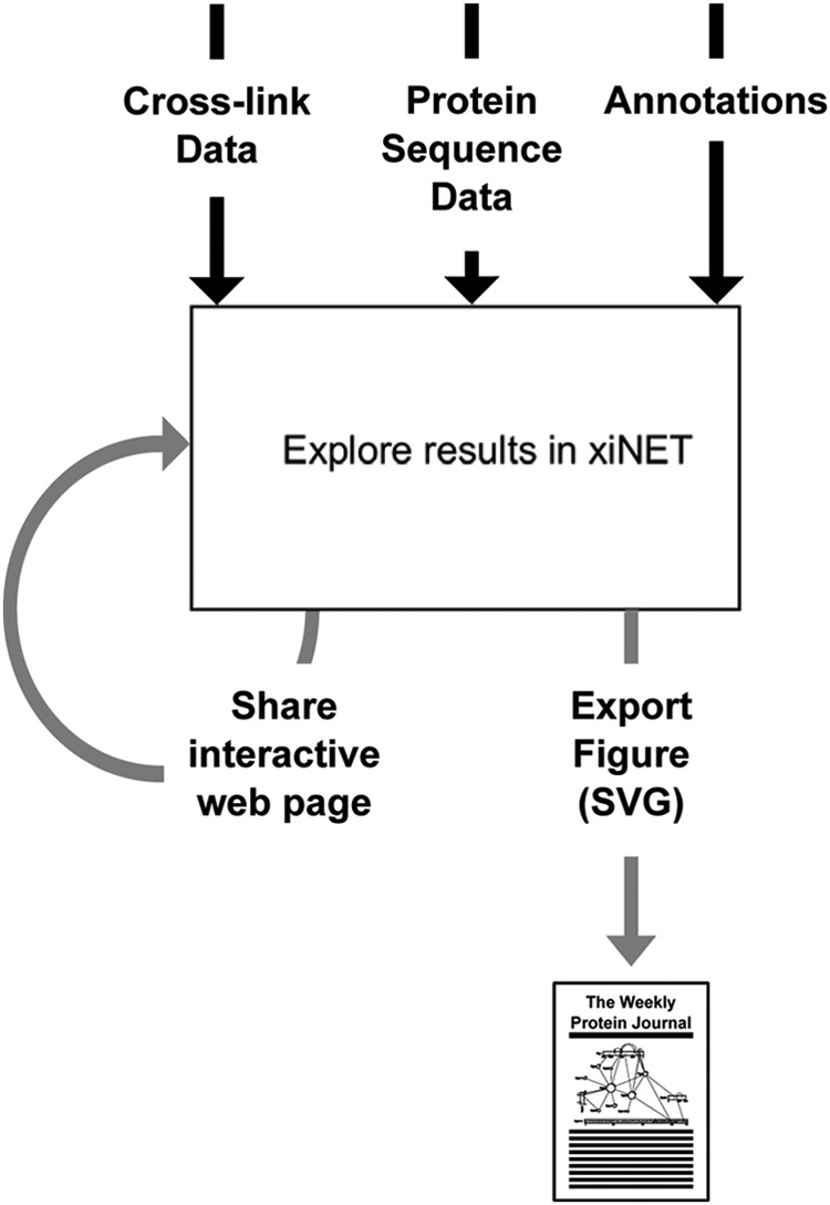
Overview of xiNET workflow. Three data sets form the input to a xiNET map: cross-link data (required); protein sequence data (can be omitted if UniProtKB accession numbers are used); and annotation data (optional, will be downloaded automatically if UniProtKB accession numbers are used for protein identifiers). Results can be communicated either by sharing the interactive map via the web or by exporting them as vector graphics that can be edited for use in publications.

Data can be loaded into xiNET by uploading it to our website or by downloading the software and running it locally. Step-by-step examples of both these use-cases are given in the case studies contained in the Results section below. When used locally, xiNET does not transmit any of the user's data across the network. A lab integrating xiNET into its workflow can thus retain control of all data used and whether or when to make data public.

To use xiNET as a web-service, data files are uploaded to http://crosslinkviewer.org/upload.html, (full instructions and details of the file formats are given there). Users are redirected to a unique URL displaying their data. Sharing an interactive figure is then as simple as sharing that URL.

The input file format of xiNET for CLMS data is a comma separated values (CSV) file. We will refer to the specific CSV format xiNET consumes as “CLMS-CSV.” This format is described at http://crosslinkviewer.org/upload.html#CLMS-CSV. It follows the structure of the data tables typically found in the supplementary information that accompanies cross-linking papers, for examples see (1, 2, 19). It is also similar to the tab delimited input format for Xlink:DB (24) and the output format of XQuest (25). CSV files are the current de facto standard for CLMS data and the different file formats can be easily interconverted. However, the standards compliant input and output for all these and similar tools would be PSI-MI (10) and we are working toward using this input.

xiNET is designed to allow its use as a component that laboratories can integrate into their work-flow by linking it directly to their own CLMS database. In essence, data can be loaded into xiNET by iterating through database results and producing calls to JavaScript functions named “addProtein” and “addMatch.”

RESULTS

With xiNET we provide a tool that summarizes CLMS results in an interactive map. This tool is an open source project at GitHub and thus can be used and further developed by any interested party. The tool can be used directly through a web page at http://crosslinkviewer.org or used locally without transmitting the data. The user controls for the interactive maps (panning, zooming, rearranging the graphical elements) are given in Table I.

Table I. User controls on xiNET linkage map (version 1.0.0).

Action	Control
Toggle the proteins between bar and circle graphical form	Left-click on protein
Zoom	Mouse wheel on background
Pan	Left-click and drag on background
Move protein	Click and drag on protein
Cycles through different bar lengths (largest length displays protein sequence)	Shift+left-click
Rotate bar	Click and drag on handles that appear at end of a protein bar when mouse is moved nearby
Grey out/show protein (and hide/show all its links)	Right-click on protein
Hide links between two specific proteins	Right-click on any link between those proteins
Show all hidden links	Right-click on background
Flip side of bar on which self-links are shown	Right-click on self-links link
Select protein or link (and further detail shown in separate panel in web page)	Left-click protein or link
Clear selection	Left-click on background
Protein details (ID, name)	Mouse hover over protein (tool-tips)
Protein-protein link details (ID, number of unique linkage site pairs, total number of supporting matches)	Mouse hover over protein-protein link (tool-tips)
Residue-level link details (ID, total number of supporting matches, linked peptides)	Mouse hover over residue level link (tool-tips and linked peptides highlighted in bars)

In this section, we provide detailed instructions for creating a xiNET map by uploading data to the website (Uploading Data to Website) or, to keep all data fully within the user's control, by using the tool locally (Local Use). We show these maps and then (Further Examples) briefly introduce other examples needed to illustrate all the features of xiNET. Fig. 3 shows the default legend for xiNET, which is used in the output shown.

Fig. 3.

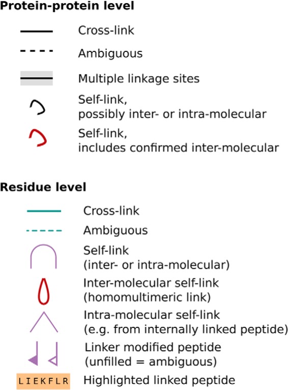
Default key for xiNET figures. Any of the lines representing links may be dashed to indicate the link is ambiguous regarding linkage site. Note that self-links can be ambiguous regarding whether they are intra or intermolecular. The default key can be modified by users/developers to adapt it to their specific representation needs. Typically, such modifications involve assigning line color to an attribute of the cross-links, for example quantitation or confidence attributes.

Uploading Data to Website

Creating a figure such as that shown in Fig. 1A manually in a drawing tool is a laborious process; xiNET removes this manual labor. In what follows, we describe how to automatically generate an interactive version of Fig. 1A from the supplementary data accompanying the original publication and annotate it with the domains described therein. Chen et al. (1) summarizes the identified linkage site pairs, omitting the peptide sequence information, in an .xls file.

To recreate the figure from the .xls file, we made a CLMS-CSV file in the following way

1. Open the .xls file in spreadsheet software,

2. Delete rows containing low confidence links or links outside TFIIF, as these are not shown in the original figure,

3. Save the result as a CSV file,

4. Edit the column headings (row 1) to match those given at http://crosslinkviewer.org/upload.html#CLMS-CSV

5. Use find-and-replace in a text editor to swap the informal protein names for UniProtKB accession numbers.

Because the file uses accession numbers as identifiers there is no need to provide sequence data. An alternative to step 5 would be to provide sequence data in a FASTA file containing the informal names used as identifiers. The domain annotation data is extracted from the original paper's text and recorded in the CSV format described at http://crosslinkviewer.org/upload.html#Annotations.

Both the CLMS-CSV file and annotation CSV file are then uploaded. The result is shown in Fig. 4. An online, interactive version is available at http:/crosslinkviewer.org/figure4.html.

Fig. 4.

TFIIF dimerization domain. Here we see xiNET displaying the data from Fig. 1, this time with self links included. xiNET uses the same numbered bar representation as is found in a variety of cross-linking publications (1, 17, 18, 19). A homomultimeric link (in red) occurs in the data set and xiNET highlights this - this link does not actually help support the conclusions of the original paper and it may be a false identification. The interactive figure can be viewed at http://crosslinkviewer.org/figure4.html.

The output in Fig. 4 shows another feature of xiNET - identifying homomultimeric links. There is a link in the data (from Tfg2, residue 279 to Tfg2, residue 279) which, if true, could only be intermolecular and could only come from a homomultimer. xiNET recognizes this and highlights it.

Local Use

Bui et al. (19) investigated the human nuclear pore complex with CLMS. They have provided us with XQuest (25) output regarding this complex for use as example data and this data contains all three cross-linking reaction product types.

We prefer the CLMS-CSV format to the XQuest output format because CLMS-CSV stores peptide sequences and link positions within peptides as separate columns. XQuest output concatenates this information together and records it as the identifier. However, for the convenience of XQuest users, xiNET reads XQuest output directly as it is very similar to its own CLMS-CSV format. Fig. 5 describes how the different product types are recorded in CLMS-CSV, though they can also be read from XQuest output directly.

Fig. 5.

The encoding of cross-linking reaction product types in xiNET's CLMS-CSV file format. xiNET displays and distinguishes all three cross-linking reaction product types, these are: A, linker modified peptides; B, internally linked peptides; and, C, cross-linked peptides. The tables show the input data for the example above it. In the input data, the product type is indicated by the presence or absence of information for the second protein and second link position. xiNET also identifies a subset of cross-linked peptides, D homomultimer links, in which the peptides overlap in the protein sequence. The overlapping region is highlighted in red. The tables also include examples in which peptide sequence information is omitted—in this case the columns LinkPos1 and LinkPos2 give the absolute position of the linkage site in the protein sequence. To record ambiguous linkage sites the values in the required columns are made into comma separated lists of alternatives. Note that peptide-level ambiguity must be treated differently depending on whether the product type is an internally linked peptide, B, or cross-linked peptides, C.

What follows describes the process of producing the interactive figure while keeping the cross-link data confidential

1. Download the xiNET project from https://github.com/colin-combe/crosslink-viewer/archive/master.zip,

2. Unzip it,

3. Place the CSV file in demo/data/MyData.csv,

4. Change the filename given in line 140 of demo/Demo.html from “demo/data/PolII.csv” to “demo/data/MyData.csv”

5. Open demo/Demo.html in a browser, (changes to the browser's security settings may be required to allow it to read files from the local disk, this security restriction does not apply if the files are served by a locally running web server).

Network traffic is generated as sequences and annotations are downloaded but the cross-link data does not leave the local machine. The results are shown in Fig. 6, in which we see xiNET displaying and distinguishing all three product types. The live version of the figure is at http://crosslinkviewer.org/figure6.html.

Fig. 6.

Example containing all three product types. The data pertains to the Human Nuclear Pore Complex, see Bui et al. (19), and xiNET distinguishes the three different product types present in the data. Note also, that the size of a circular node scales with the length of the protein sequence such that doubling the length of a protein leads to doubling the area of a circle. The interactive figure can be viewed at http://crosslinkviewer.org/figure6.html.

Further Examples

Two further examples are now shown, in order to cover all the features of xiNET described in the preceding “Benefits of xiNET” section.

Fig. 7 shows ambiguous data displayed in xiNET. Dashed lines are used to indicate the ambiguous links and highlights on mouse-over show the possible alternatives. In Fig. 7 the numbered bars have been expanded (see Table I for user controls) until the sequence of the protein is visible. When xiNET has information on the peptide sequence, its highlights both the link and the linked peptide on mouse-over. Hence, in Fig. 7 we can see the specific recurring peptide that is the source of ambiguity. (Interactive figure at http://crosslinkviewer.org/figure7.html.)

Fig. 7.

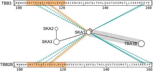
Example of ambiguous CLMS results. Ambiguity regarding the linkage site can occur if, for example, an identified cross-linked peptide belongs to more than one protein in the search space. xiNET uses a dashed line to represent ambiguous linkage sites while highlights on mouse-over are used to show the possible alternatives. The example data shows cross-links between microtubules and the human kinetochore Ska complex (18). The links from SKA1 to residues in the 110–120 range of Tubulin beta-3 chain isoforms TBB3 and TBB2B are all ambiguous; the same identified peptide (highlighted in orange) occurs in both isoforms. The links from SKA1 to residues around 160 in TBB3 and TBB2B are all unambiguous; for these links, all the identified peptides contained residue 155, which distinguishes TBB3 and TBB2B. In the interactive figures (for example http://crosslinkviewer.org/figure7.html), the peptide attached to a particular cross-link is highlighted in orange when the mouse is moved over a link and the highlight is accompanied by a tool-tip giving protein names or ID's, linked residue numbers and the number of supporting peptide-spectrum matches.

Fig. 8 illustrates a further aspect of xiNETs representation of sequence features such a domains. (Interactive figure at http://crosslinkviewer.org/figure8.html.) When proteins are shown as numbered bars, the domains are marked as colored regions along this bar. When the nodes are collapsed into a circle, domain annotation information is shown on these circular nodes as sectors, the start and end angles of which correspond to the start and end residues of the domain. Because the sectors are color-coded on the basis of their domain name, homologous proteins can be recognized by similar patterns in their colored sectors.

Fig. 8.

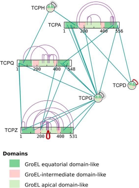
xiNET displays CLMS data in the context of other sequence information. Domains, or other annotated regions, are shown as color-coded segments of the bars or as color-coded sectors of the circles representing proteins. The start and end angles of a sector correspond to the start and end residues of the domain (residue 1 is at 12 o'clock). The data is a subset of the data from Herzog et al. (2). A live example containing the whole dataset can be seen at http://crosslinkviewer.org/figure8.html.

DISCUSSION

A key feature of xiNET's user interface is its ability to toggle interactor nodes between a bar (residues shown) and a circle (interactions aggregated to protein level). This allows the user to select which parts of the network are simplified and which have more detail displayed. One aspect of xiNET is therefore that it provides a hierarchical graph. This is similar to Visant (9), though Visant does not use an axis representing the sequence for positioning residue-level nodes.

We hope that our work will facilitate the spread of CLMS as an analytical technology by simplifying and enhancing the way researchers explore and share the information provided by this type of experiment. This includes the possibility of sending interactive figures to colleagues and journals as html addresses for pages containing xiNET. We aspire to the creation of a common visual language for communicating CLMS results. The open availability of xiNET increases the chances that its use may even become standard across the field, avoiding a duplication of development efforts which would divert resources away from the biological questions we seek to answer.

xiNET does not cater for all our needs when visualizing aspects of CLMS data. Three types of figure are commonly found in CLMS publications: spectra annotated for human inspection, cross-links visualized on a three-dimensional structure, and a two-dimensional graphical summary of identified cross-links. These correspond to three types of view required in a complete system for the visualization and downstream analysis of CLMS data. xiNET is a component providing one of these views—the summary of identified cross-links. Software for the purpose of visualizing annotated spectra that already exists, for example, MSViewer (26) and xiSPEC at http://spectrumviewer.org/. Xlink:DB (24) contains a three-dimensional structure viewer intended for use with CLMS data. xiNET provides a very efficient way of navigating CLMS data and we therefore anticipate it will play a central role in an integrated platform that makes all aspects of CLMS experiments explorable in an interconnected way.

The maps that xiNET displays could be further developed to include different types of bio-molecule, such as DNA, RNA or small molecules. The technique of toggling the representation of polymer interactors between bar and circle could be applied to the visualization of any experimental data in which interactions are identified between specific regions of sequences. Both these things, expanding the range of types of molecule and the range of types of experimental data, are part of developing xiNET into a general viewer for bio-molecular interactions, see http://interactionviewer.org.

REFERENCES

- 1. Chen Z. A., Jawhari A., Fischer L., Buchen C., Tahir S., Kamenski T., Rasmussen M., Lariviere L., Bukowski-Wills J. C., Nilges M., Cramer P., Rappsilber J. (2010) Architecture of the RNA polymerase II–TFIIF complex revealed by cross-linking and mass spectrometry. EMBO J. 29, 717–726 [DOI] [PMC free article] [PubMed] [Google Scholar]
- 2. Herzog F., Kahraman A., Boehringer D., Mak R., Bracher A., Walzthoeni T., Leitner A., Beck M., Hartl F. U., Ban N., Malmström L., Aebersold R. (2012) Structural probing of a protein phosphatase 2a network by chemical cross-linking and mass spectrometry. Science 337, 1348–1352 [DOI] [PubMed] [Google Scholar]
- 3. Zheng C., Yang L., Hoopmann M. R., Eng J. K., Tang X., Weisbrod C. R., Bruce J. E. (2011) Cross-linking measurements of in vivo protein complex topologies. Mol. Cell. Proteomics 10, M110.006841–M110.006841 [DOI] [PMC free article] [PubMed] [Google Scholar]
- 4. Gehlenborg N., Wong B. (2012) Points of view: Networks. Nat. Methods 9, 115. [DOI] [PubMed] [Google Scholar]
- 5. Seebacher J., Mallick P., Zhang N., Eddes J. S., Aebersold R., Gelb M. H. (2006) Protein cross-linking analysis using mass spectrometry, isotope-coded cross-linkers, and integrated computational data processing. J. Proteome Res. 5, 2270–2282 [DOI] [PubMed] [Google Scholar]
- 6. Gehlenborg N., O'Donoghue S. I., Baliga N. S., Goesmann A., Hibbs M. A., Kitano H., Kohlbacher O., Neuweger H., Schneider R., Tenenbaum D., Gavin A. C. (2010) Visualization of omics data for systems biology. Nat. Methods 7, S56–S68 [DOI] [PubMed] [Google Scholar]
- 7. Shannon P., Markiel A., Ozier O., Baliga N. S., Wang J. T., Ramage D., Amin N., Schwikowski B., Ideker T. (2003) Cytoscape: A software environment for integrated models of biomolecular interaction networks. Genome Res. 13, 2498–2504 [DOI] [PMC free article] [PubMed] [Google Scholar]
- 8. Barsky A., Gardy J. L., Hancock R. E., Munzner T. (2007) Cerebral: a Cytoscape plugin for layout of and interaction with biological networks using subcellular localization annotation. Bioinformatics 23, 1040–1042 [DOI] [PubMed] [Google Scholar]
- 9. Hu Z., Mellor J., Wu J., Kanehisa M., Stuart J. M., DeLisi C. (2007) Towards zoomable multidimensional maps of the cell. Nat. Biotechnol. 25, 547–554 [DOI] [PubMed] [Google Scholar]
- 10. Hermjakob H., Montecchi-Palazzi L., Bader G., Wojcik J., Salwinski L., Ceol A., Moore S., Orchard S., Sarkans U., Von Mering C., Roechert B., Poux S., Jung E., Mersch H., Kersey P., Lappe M., Li Y., Zeng R., Rana D., Nikolski M., Husi H., Brun C., Shanker K., Grant S. G., Sander C., Bork P., Zhu W., Pandey A., Brazma A., Jacq B., Vidal M., Sherman D., Legrain P., Cesareni G., Xenarios I., Eisenberg D., Steipe B., Hogue C., Apweiler R. (2004) The HUPO PSI's molecular interaction format—a community standard for the representation of protein interaction data. Nat. Biotechnol. 22, 177–183 [DOI] [PubMed] [Google Scholar]
- 11. Berman H. M., Westbrook J., Feng Z., Gilliland G., Bhat T. N., Weissig H., Shindyalov I. N., Bourne P. E. (2000) The protein data bank. Nucleic Acids Res. 28, 235–242 [DOI] [PMC free article] [PubMed] [Google Scholar]
- 12. Doncheva N. T., Assenov Y., Domingues F. S., Albrecht M. (2012) Topological analysis and interactive visualization of biological networks and protein structures. Nat. Protoc. 7, 670–685 [DOI] [PubMed] [Google Scholar]
- 13. Martin A. J., Vidotto M., Boscariol F., Di Domenico T., Walsh I., Tosatto S. C. (2011) RING: networking interacting residues, evolutionary information and energetics in protein structures. Bioinformatics 27, 2003–2005 [DOI] [PubMed] [Google Scholar]
- 14. Swint-Kruse L., Brown C. S. (2005) Resmap: automated representation of macromolecular interfaces as two-dimensional networks. Bioinformatics 21, 3327–3328 [DOI] [PubMed] [Google Scholar]
- 15. Lasker K., Förster F., Bohn S., Walzthoeni T., Villa E., Unverdorben P., Beck F., Aebersold R., Sali A., Baumeister W. (2012) Molecular architecture of the 26S proteasome holocomplex determined by an integrative approach. Proc. Natl. Acad. Sci.USA 109, 1380–1387 [DOI] [PMC free article] [PubMed] [Google Scholar]
- 16. Krzywinski M., Birol I., Jones S. J., Marra M. A. (2011) Hive plots–rational approach to visualizing networks. Briefings Bioinformatics 13, 5. bbr069–644 [DOI] [PubMed] [Google Scholar]
- 17. Jennebach S., Herzog F., Aebersold R., Cramer P. (2012) Crosslinking-MS analysis reveals RNA polymerase I domain architecture and basis of rRNA cleavage. Nucleic Acids Res. 40, 5591–5601 [DOI] [PMC free article] [PubMed] [Google Scholar]
- 18. Abad M.A., Medina B., Santamaria A., Zou J., Plasberg-Hill C., Madhumalar A., Jayachandran U., Redli P.M., Rappsilber J., Nigg E.A., Jeyaprakash A.A. (2014) Structural basis for microtubule recognition by the human kinetochore Ska complex. Nat. Commun. 5, 2964. [DOI] [PMC free article] [PubMed] [Google Scholar]
- 19. Bui K. H., von Appen A., DiGuilio A. L., Ori A., Sparks L., Mackmull M. T., Bock T., Hagen W., Andrés-Pons A., Glavy J. S., Beck M. (2013) Integrated Structural Analysis of the Human Nuclear Pore Complex Scaffold. Cell 155, 1233–1243 [DOI] [PubMed] [Google Scholar]
- 20. Bostock M., Ogievetsky V., Heer J. (2011) D3: Data-Driven Documents. IEEE Trans Visualization Computer Graphics 17, 2301–2309 [DOI] [PubMed] [Google Scholar]
- 21. The UniProt Consortium (2013) Update on activities at the Universal Protein Resource (UniProt) in 2013. Nucleic Acids Res. 41, D43–D47 [DOI] [PMC free article] [PubMed] [Google Scholar]
- 22. Gough J., Karplus K., Hughey R., Chothia C. (2001) Assignment of homology to genome sequences using a library of hidden Markov models that represent all proteins of known structure. J. Mol. Biol. 313, 903–919 [DOI] [PubMed] [Google Scholar]
- 23. Dowell R. D., Jokerst R. M., Day A., Eddy S. R., Stein L. (2001) The distributed annotation system. BMC Bioinformatics 2, 7. [DOI] [PMC free article] [PubMed] [Google Scholar]
- 24. Zheng C., Weisbrod C. R., Chavez J. D., Eng J. K., Sharma V., Wu X., Bruce J. E. (2013) xlink:DB: Database and software tools for storing and visualizing protein interaction topology data. J. Proteome Res. 12, 1989–1995 [DOI] [PMC free article] [PubMed] [Google Scholar]
- 25. Rinner O., Seebacher J., Walzthoeni T., Mueller L. N., Beck M., Schmidt A., Mueller M., Aebersold R. (2008) Identification of cross-linked peptides from large sequence databases. Nat. Methods 5, 315–318 [DOI] [PMC free article] [PubMed] [Google Scholar]
- 26. Baker P. R., Chalkley R. J. (2014) MS-viewer: a web-based spectral viewer for proteomics results. Mol. Cell. Proteomics 13, 1392–1396 [DOI] [PMC free article] [PubMed] [Google Scholar]