Predictors of intra-community variation in air quality

Abstract

Air quality has emerged as a key determinant of important health outcomes in children and adults. This study aims to identify factors that influence local, within-community air quality, and to build a model for traffic-related air pollution (TRP).We utilized concentrations of NO₂, NO, and total oxides of nitrogen (NO_x), which were measured at 942 locations in 12 southern California communities. For each location, population density, elevation, land-use, and several indicators of traffic were calculated. A spatial random effects model was used to study the relationship of these predictors to each TRP.Variation in TRP was strongly correlated with traffic on nearby freeways and other major roads, and also with population density and elevation. After accounting for traffic, categories of land-use were not associated with the pollutants. Traffic had a larger relative impact in small urban (low regional pollution) communities than in large urban (high regional pollution) communities. For example, our best fitting model explained 70% of the variation in NO_x in large urban areas and 76% in small urban areas. Compared with living at least 1,500m from a freeway, living within 250m of a freeway was associated with up to a 41% increase in TRP in a large urban area, and up to a 75% increase in small urban areas.Thus, traffic strongly affects local air quality in large and small urban areas, which has implications for exposure assessment and estimation of health risks.

Introduction

Air quality in the urban environment has emerged as an important determinant of human health. Increased levels of air pollution have been linked to health effects in childhood, including reduced lung development (Gauderman et al., 2004, 2007) and increased risk of asthma (McConnell et al., 2002, 2006) and respiratory symptoms (Dockery et al., 1996; McConnell et al., 1999, 2003). Air pollution has also been associated with adverse adult health effects, including cardiovascular (Peters, 2009) and respiratory disease (Gotschi et al., 2008), and mortality (Dockery et al., 1993). Many of these findings have been based on ecological studies that compared the health of residents in high-pollution communities to that of residents in low-pollution communities. A number of studies have demonstrated that intra-community indicators of local air quality, often determined by proximity to major roadways, are associated with adverse health outcomes (Edwards et al., 1994; Brunekreef et al., 1997; Hirsch et al., 1999; Venn et al., 2000, 2001; Brauer et al., 2002; Delfino, 2002; Nicolai et al., 2003; Kim et al., 2004; Zmirou et al., 2004; Gauderman et al., 2005, 2007; McConnell et al., 2006). To better understand these associations, it is important to describe how air quality varies by roadway proximity and other factors in order to develop models for predicting traffic-related air pollutant levels for use in health-related research.

There is a significant amount of small-scale variability in air pollution concentrations around roadways. For example, Zhu et al. (2002) showed that carbon monoxide, particle number, and black carbon were substantially higher near a busy interstate freeway in southern California, with levels dropping sharply within a few hundred meters from the roadway during daytime hours. Levels of NO₂ have also been shown to be highest near a busy road and declining gradually with increasing distance (Gilbert et al., 2003; Beckerman et al., 2008; Dijkema et al., 2010; Skene et al., 2010). Most studies of intra-community air quality have been based on extensive monitoring in a single city (Hoek et al., 2008) or on a few monitors in each of many cities (Hart et al., 2009).

In this study, we measured concentrations of trafficrelated pollutants (TRP), including nitrogen dioxide (NO₂), nitric oxide (NO), and total oxides of nitrogen (NO_x), at multiple locations within 12 southern California communities participating in the Children’s Health Study (CHS; Peters et al., 1999; McConnell et al., 2006). We developed a set of models that utilize widely available data to predict outdoor concentrations of these pollutants with the intent of assigning ambient exposure values to subjects when studying health effects related to TRP. Models were initially constructed using geographic information, including proximity to freeway and non-freeway traffic corridors, traffic volume, local elevation, population density, and land-use. In addition, we evaluated the improvement in model performance obtained by including dispersionmodeled estimates of near-road TRP that accounts for traffic volume and meteorology. As the 12 study communities vary in their regional air quality, we assessed how the effects of traffic and other variables of local air quality differed based on the general air quality of the region. Finally, we report on the potential of these models to predict air quality in communities where measurements have not been made.

Materials and methods

Study Subjects

The CHS was initiated in 1993 to investigate the long-term relationship between ambient air pollution and children’s respiratory health. The CHS is currently conducting active follow-up of its fifth cohort that was enrolled in 2002–2003 with a sample of 5603 children from kindergarten and 1st grade. These children were recruited from 13 southern California communities that varied substantially in their air quality. Details of CHS community and subject selection have been previously reported (Peters et al., 1999; McConnell et al., 2006).

Air Monitoring

In 2005–2006, we conducted an extensive air monitoring study involving active study subjects. We focused on 12 of our 13 communities (Figure 1), eliminating a mountainresort community (Lake Arrowhead) as it had relatively little local traffic. We used passive diffusion-based Ogawa samplers (Koutrakis et al., 1994) to measure levels of NO₂ and NO_x outside homes, schools, and central monitoring site locations in the 12 study communities (Supplementary Figure A online). Home sampling site locations were selected from the residences of Cohort E subjects who were participants in one of two asthma-nested case–control studies being conducted within the CHS cohort. Informed consent was obtained from a parent or guardian before sampling at a child’s home.

Figure 1.

Locations of 12 Children’s Health Study Communities in Southern California.

A total of 942 locations were monitored across the 12 communities, with each location monitored for a 2-week period in summer and a 2-week period in winter (Supplementary Figure B online). Within a given season, all locations within a study community were monitored over the same 2-week period to avoid temporal differences in air quality. Within each site, sampling was conducted at the same outdoor location in the summer and winter periods. A systematic quality assurance sampling program was included, including at least 10% co-located (duplicate) sampling, laboratory blanks, and trip blanks. For NO_x and NO₂ in both seasons, and for NO in winter, sample-duplicate Pearson correlation coefficients (r) were ≥0.99 and duplicate coefficients of variation (CV) were below 8%. For summertime NO, agreement between duplicates was lower (r = 0.97, CV = 21%), but still acceptable. All sampling filters were purchased from a commercial source (Ogawa, Pompano Beach, FL, USA), loaded and unloaded under filtered air conditions at a USC facility, and analyzed by a commercial laboratory (RTI International, Research Triangle Park, NC, USA). Outdoor concentrations of NO were determined by subtracting measured NO₂ from NO_x obtained by the same sampler.

Modeling

Geo-positional satellite (GPS) measurements were taken at the sampling location each time a passive sampler was deployed. GPS discrepancies greater than 40m between successive measurements recorded at the same location were rectified using additional tools including Google Earth and maps. Circular buffers of radius 300m were formed around each sampling location using ArcGIS 9.3 (Environmental Systems Research Institute (ESRI; Redlands, CA, USA)) and, as described below, a wide range of predictors including traffic volume, dispersion-modeled near-road TRP, population density, elevation, and land-use were calculated within these buffers. We used a common buffer size for all of our predictor variables for comparability, and based on previous studies, 300m was chosen for its appropriate spatial extent when examining traffic-related pollution (Zhu et al., 2002; Zhou and Levy, 2007; Kan et al., 2008)

Distance to Roads

The distance from sampling locations to the nearest interstate freeway or highway (FRC1), major arterial (FRC3), and minor arterial roads (FRC4) was computed using the Tele Atlas MultiNet road network data (Tele Atlas, Menlo Park, CA, USA) and ArcGIS 9.3. We used the distance to nearest freeway (FRC1) and the distance to the nearest non-freeway major road (the minimum of FRC3 and FRC4) in the statistical models.

Traffic Volume

Annual average daily traffic (AADT) volumes by roadway link were obtained from the California Department of Transportation (CALTRANS) for the year 2000. These data were transferred from the original network to the more spatially resolved TeleAtlas MultiNet network (Wu et al., 2005) and AADT volumes were projected to represent 2005 vehicle-miles-travelled (CALTRANS, 2008). Traffic density maps were created by allowing volumes to decrease by 90% from the edge to 300m (perpendicular) from the roadways (Kan et al., 2008). Using these maps, traffic density was assigned to the 300m buffer around each sampling location.

CALINE4-modeled TRP

Line source dispersion model estimates of annual average TRP concentrations were generated using the CALINE4 model (Benson, 1989). The principle inputs to CALINE4 were surface wind data for 2001–2005 for each community, the link-based AADT volume data for all road classes (i.e., FRC1- FRC6) in each community, and vehicle emission factors for 2005 in the South Coast, South Central Coast, and San Diego Air Basins from the EMFAC2007 model (CARB, 2007). Diurnal traffic volume variations and day-of-week variations for light-duty and heavy-duty vehicles on freeways were obtained by averaging CALTRANS weigh-in-motion data for southern California. Diurnal variations for arterials and collectors were determined from more limited traffic measurements (Chinkin et al., 2002). The contribution of vehicle traffic on interstate freeways and highways (CALINE4 freeway TRP), and arterials and collectors (CALINE4 non-freeway TRP) were computed separately. We scaled CALINE4 output to NO_x, which can be viewed as an indicator for the complex TRP mixture near roads.

Population Density

Population density data at the block group level were obtained from US Census Bureau (2000 data projected to year 2005) via ESRI’s data repository We calculated the ratio of the area of the block group within the buffer to the total area of the block group within each 300m buffer. We then multiplied this ratio by the assigned population for that block group, and accumulated these over all buffer sections to obtain the total population density.

Elevation

Elevation data were obtained from the US Geological Survey (USGS) website (http://seamless.us.gov) using National Elevation Data with ~30m resolution. We computed the mean (E_n) and standard deviation (s_n) of the 30m-grid elevation values within each 300m buffer, and the overall mean elevation (E_c) of each study community. We considered three elevation variables in our air quality models, including (1) the neighborhood (within buffer) elevation relative to the community (E_n−E_c), (2) the elevation variability of each neighborhood (s_n), and (3) the elevation of each sampling location (E_i) relative to the neighborhood (i.e., E_i−E_n).

Land-Use Categories

Eight of the twelve study communities were located in the Los Angeles (LA) basin where land use was well characterized by the Southern California Association of Governments (SCAG). SCAG provides a total of 133 possible land-use categories, which we aggregated into eight categories: commercial, industrial, utilities, transportation, residential, agricultural, water bodies, and open space. For each sampling location covered by SCAG, we computed the percentage of area within the 300-m buffer attributed to each of these eight landuse categories.

Statistical Methods

The outcome data consisted of two 2-week integrated concentrations of NO₂, NO, and NO_x for a total of 942 locations across the 12 study communities. We computed the average of summer and winter concentrations recorded at each location. The CHS communities were originally chosen for having a wide range in air quality. In this work, however, we focused on factors that affect local air quality within each of the communities, and how the factors that affect local variation depend on general air quality of the region. Let Y_ci denote the natural log of the measured concentration of a given pollutant (NO₂, NO, or NO_x) at location i (e.g., a home) in community c (c = 1, … ,12), and let Y_c denote the mean of Y_ci for all measured locations in community c. Natural log transformations were applied to each measured pollutant to satisfy linear-regression modeling assumptions of normality and homoscedasticity. The outcome variable used in all regression models was of the form D_ci = Y_ci−Y_c, that is, the difference between the log concentration at location i and the corresponding community mean. Let D denote the vector of differences for all sampling locations; note that the use of these deviations as the outcome focused our models on factors affecting local variation in air quality.

Correlation coefficients and linear regression models were used to explore relationships of D with each predictor variable. Stepwise linear regression with a significance threshold of 0.15 was used to determine the best predictors chosen from the set of traffic variables (distances, volumes, CALINE4-modeled TRP), squared versions of each traffic variable, elevation, population density, and land-use categories. This ‘fixed-effects’ model can be denoted D = βX(s) + ε, where X(s) is the set of predictors at geographic locations s and ε are residuals assumed to be independent and normally distributed.

We then addressed potential within-community residual spatial correlation that may not have been completely accounted for by the predictor variables by introducing a spatial covariance function. This resulted in a mixed model of the form D = βX(s) + Z(s) + ε, where Z(s) is spatial random effects assumed to be normally distributed with variancecovariance matrix σ²G(θ). Spatial dependence was parameterized by G(θ), a function of distance z_ij between locations s_i and s_j. Exploratory analyses of several covariance functions including exponential, Gaussian, spherical, and Matern, indicated that the exponential covariance structure was efficiently computed and provided a good fit to our data (Waller and Gotway, 2004). The spatial random effects model was estimated by maximum likelihood and we compared the fit of this model to the fixed-effects model using a likelihood ratio test (LRT). We also used correlograms to graphically examine the spatial correlation in the residuals before and after accounting for spatial random effects. The correlogram plots the correlation between model residuals at locations s_i and s_j against the distances z_ij.

Effect estimates were scaled to the percent change in local air pollutant concentration per increase of one interquartile range (IQR) of the corresponding predictor. This approach to scaling effect estimates facilitates direct comparison of the relative impact of each predictor on each pollutant. In some analyses, study communities were categorized as ‘within the LA basin’ or ‘outside the LA basin’ to capture regional-scale differences in air quality. Appropriate interaction terms were considered to test whether the effect of traffic and other factors on local pollutant variation was modified by regional air quality. To evaluate the fit of our models, we performed standard 10-fold cross-validation using stratified random sampling to ensure that a representative number of observations from each community were included in each crossvalidation sample. We also performed leave-one-community out cross-validation to evaluate how well our models might perform at estimating local variation in unmeasured communities.

We used our final models to compute predicted concentrations of NO₂, NO, and NO_x at each sampling location. Our model provides estimates of relative pollutant levels within a community. To transform these relative levels into absolute concentrations, we applied our predictions to a typical urban community in the LA basin and to a typical small urban community outside the LA basin. ‘Typical’ for each was defined as having regional levels of NO₂, NO, and NO_x equal to the mean levels in our ‘in-basin’ and ‘out-of-basin’ study communities. We then computed the mean of the predictions by categories of distance to freeway (<250 m, 250–500 m, 500–1,500 m, and >1,500 m) and distance to non-freeway major roads (<75 m, 75–150 m, 150–300 m, and >300 m). These mean predictions provide estimates of the overall impact of road proximity on pollutant levels, accounting for population density, elevation, and other model predictors, in both large and small urban communities.

Results

In all communities, there was substantial variation in concentrations of NO₂, NO, and NO_x across sampling locations (Figure 2). The community-average concentrations of NO₂ and NO (Table 1) ranged from a low of 5.0 to 4.5 p.p.b., respectively (Santa Maria), to a high of 30.4 (NO₂, San Dimas) and 49.3 p.p.b. (NO, Anaheim). Average concentrations of total NO_x ranged from 9.6 to 79.1 p.p.b. In general, the eight study communities within the LA basin had significantly higher levels of NO₂, NO, and NO_x compared with the four study communities outside the basin. However, the four communities outside the basin generally had larger CV for all three pollutants, suggesting a greater degree of relative spatial variation in these lower-pollution areas compared with the more polluted basin communities.

Figure 2.

Four-week average levels of measured NO₂, NO, and NO_x at sampling locations within each study community.

Table 1.

Pollutant levels measured at 942 locations across 12 study communities.

Community	Number of locations	Pollutanta
		NO2		NO		NOx
		Mean	CV (%)	Mean	CV (%)	Mean	CV (%)
Within LA basin
Mira Loma (MRL)	80	18.5	13.2	9.7	24.2	28.2	14.3
Riverside (RIV)	100	20.6	18.6	16.0	59.7	36.4	34.7
Upland (UPL)	103	25.5	25.6	18.6	57.8	44.2	37.6
Glendora (GLE)	100	25.8	14.1	20.5	41.6	46.3	24.6
San Bernardino (SBE)	66	25.8	14.7	15.6	35.0	41.2	21.1
Long Beach (LGB)	71	25.9	9.6	46.9	15.8	72.4	12.7
Anaheim (ANA)	61	29.8	8.4	49.3	18.4	79.1	14.0
San Dimas (SDM)	77	30.4	7.5	31.8	22.5	62.3	14.2
Mean		25.3	21.3	26.0	62.3	51.3	39.0
Outside LA basin
Santa Maria (SMA)	67	5.0	18.8	4.5	30.2	9.6	22.1
Alpine (ALP)	72	10.9	38.7	4.8	99.6	15.7	56.3
Lake Elsinore (LKE)	72	10.9	19.2	7.3	38.0	18.2	25.9
Santa Barbara (SBA)	73	11.1	29.2	14.9	59.1	26.3	45.4
Mean		9.5	39.8	7.9	84.0	17.5	55.3

^aMean and coefficient of variation (CV) across sampling locations within each study community of the 4-week average concentrations of each pollutant (p.p.b.).

Pollutant concentrations were univariately correlated with several traffic and land-use indicators (Table 2). For example, the strongest Pearson correlations (r) with measured NO_x were observed with CALINE4-modeled TRP from freeways (r = 0.68, P<0.0001) and non-freeways (r = 0.62, P<0.0001). Measured NO_x was also correlated with distance to freeways (r = −0.40, P<0.0001), traffic volume within a 300-m buffer of the sampling location (r = 0.47, P<0.0001), and average neighborhood elevation relative to the rest of the community (r = −0.45, P<0.0001). Similar trends were observed for NO and NO₂. Pollutant concentrations were weakly correlated with SCAG land-use categories, in patterns that one might expect.

Table 2.

Univariate correlation coefficients of measured pollutants with several variables.

Predictor	Pollutant
	NO2	NO	NOx
Distance
Nearest freeway	−0.42***	−0.35***	−0.40***
Nearest non-freeway major road	−0.35***	−0.22***	−0.29***
Traffic volume
Nearest freeway	0.31***	0.22***	0.26***
Nearest non-freeway major road	0.38***	0.29***	0.33***
Within 300m buffer	0.41***	0.46***	0.47***
CALINE-modeled TRP
From freeways	0.70***	0.60***	0.68***
From non-freeway major roads	0.67***	0.54***	0.62***
Population density (300m buffer)	0.29***	0.26***	0.29***
Elevation
Neighborhood relative to community	−0.50***	−0.39***	−0.45***
Home relative to neighborhood	−0.03	−0.05	−0.05
Local standard deviation	−0.25***	−0.21***	−0.24***
Land-use categories
Agriculture	−0.03	−0.05	−0.06
Commercial	0.23***	0.11**	0.16***
Industrial	0.09*	0.04	0.05
Open-space	−0.08*	−0.02	−0.04
Transportation	0.19***	0.25***	0.25***
Utilities	−0.13**	0.02	−0.02
Water-bodies	−0.06	−0.04	−0.05
Residential	−0.13***	−0.12**	−0.13**

Correlation coefficients for land use variables are restricted to the eight communities with compete land-use data.

^*P<0.05;

^**P<0.005;

^***P<0.0005.

Focusing on the nine communities with complete land-use data, traffic-related variables, and elevation were important predictors of local pollutant levels (Table 3). For instance, the 10-fold cross-validation R-squared (R²) values for NO_x were 24% based on a model that included distances to nearby major roads (freeways and non-freeways, Model 1), 23% in a model that included traffic volumes on nearby roads (Model 2), and 34% that included our three elevation variables (Model 3). When modeled alone, population density and land-use did not explain much variability in NO_x (R² = 5%, Models 4, 5). Models including distances to roads, elevation, and population density resulted in R² = 53% (Model 6) and adding land-use categories to this model did not explain any additional variability (R² = 53%, Model 7). On the other hand, Model 6 was substantially improved with the addition of traffic volume on nearby roads (R² = 63%, Model 8). To determine the usefulness of including dispersion model estimates in the model, we note that when included alone, freeway and non-freeway CALINE4 TRP had a very strong relationship with the pollutants (R² = 67%, Model 9). The model including covariates for CALINE4 TRP, distances to roads, traffic volume, elevation, and population provided the best general fit for all three pollutants (R² = 68% for NO₂, 61% for NO, and 71% for NO_x, Model 11). This model was not improved (and for NO₂ was worse) with the addition of land-use variables (Model 12).

Table 3.

10-fold cross-validation R² values from a variety of models based on the eight study communities with complete land-use data.

Model	Predictorsa	Pollutant
		NO2	NO	NOx
1	Distances	0.24	0.19	0.24
2	Volume	0.20	0.22	0.23
3	Elevation	0.32	0.31	0.34
4	Population density	0.04	0.05	0.05
5	Land-use categories	0.08	0.03	0.05
6	Distance, elevation, population	0.51	0.45	0.53
7	Distance, elevation, population, land use	0.50	0.46	0.53
8	Distance, volume, elevation, population	0.63	0.55	0.63
9	CALINE-modeled TRP	0.65	0.59	0.67
10	CALINE-modeled TRP, distance, elevation, population	0.66	0.61	0.70
11	CALINE-modeled TRP, distance, volume, elevation, population	0.68	0.61	0.71
12	CALINE-modeled TRP, distance, volume, elevation, population, land use	0.67	0.61	0.71

^aEach set of predictors includes all of the variables listed in Table 2 under the respective heading. Squares of the distance and volume variables were also considered. Stepwise selection was used to obtain the best subset of predictors for each model.

The model with simple GIS variables (Model 8) is highly comparable to one that incorporates the more complicated dispersion model variables (Model 9). Based on data from all 12 study communities we found similar results, with the CALINE4 only model having R² = 0.66 and the model with only GIS variables having R² = 0.60. However, our best fitting model had 10-fold cross-validation R² values of 71%, 64%, and 71% for NO₂, NO, and NO_x, respectively, when all 12 communities were included. The corresponding leaveone- community out R² values were 60%, 61%, and 71%, suggesting that these models would also do a good job of predicting local variation in a new, unmeasured community. With this model, we found that an increase of one IQR in CALINE4-modeled TRP from freeways was related to an 8.8% increase in local NO₂ concentrations, a 19.6% increase in NO, and a 13.4% increase in local NO_x (Table 4). Slightly smaller effects were observed for CALINE4 TRP from a non-freeway major road, and elevation also had an important (negative) impact on near-road pollution. In the absence of available dispersion modeling, the model containing only GIS variables proved to be very good at predicting nitrogen oxides. Distance to nearest freeway was the most important predictor as it resulted in an 8.2%, 12.7% and 12.4% decrease in NO₂, NO, and NO_x, respectively (Table 5). Elevation again had an important negative impact on these concentrations, and traffic density had an important positive impact resulting in a 3.7%, 10.8% and 6.3% increase in NO₂, NO, and NO_x, respectively.

Table 4.

Percent change in pollutant level per increase of one interquartile range (IQR) in the indicated predictor based on analysis of all 12 communities.

Predictor variable	NO2	NO	NOX
	% Change	% Change	% Change
CALINE-modeled TRP (freeway)	8.8***	19.6***	13.4***
CALINE-modeled TRP (non-freeway)	4.7***	16.8***	10.4***
Distance to nearest freeway	−2.0*	−2.9*	−4.0***
Squared distance to nearest freeway	0.4	1.1*	1.0*
Distance to nearest non-freeway major road	−1.9***	−2.4***	−2.4***
Non-freeway traffic volume within a 300m buffer	1.1**	−0.5	0.0
Population within a 300m buffer	1.5***	2.7**	2.3***
Neighborhood elevation relative to the community	−3.5***	−6.8***	−4.9***
LRT fixed versus spatial model	437.8***	485.3***	596.8***
10-fold cross-validation R2	71%	63%	71%

The IQRs are 1.9U (scaled to p.p.b. of NO_x) of freeway TRP, 1.6U non-freeway TRP, 1.2 km distance to the nearest freeway, 0.88 km of freeway distance squared, 0.36 km distance to the nearest non-freeway major road, 0.31U of volume in a 300m buffer, 371 people per km², and 41m in a neighborhood elevation relative to the mean community elevation.

^*P<0.05;

^**P<0.005;

^***P<0.0005.

Table 5.

Percent change in pollutant level per increase of one IQR in the indicated predictor based on analysis of all 12 communities and GIS only model (no dispersion model).

Predictor variable	NO2	NO	NOX
	% Change	% Change	% Change
Distance to nearest freeway	−8.2***	−12.7***	−12.4***
Squared distance to nearest freeway	0.9**	1.9*	1.4**
Distance to nearest non-freeway major road	−2.5***	−5.3***	−3.3***
Non-freeway traffic volume within a 300m buffer	−2.4***	3.0**	0.7
Traffic density decay in 300m buffer	3.7***	10.8***	6.3***
Squared traffic density decay in 300m buffer	1.1***	4.5***	2.6***
Population within a 300m buffer	1.2***	1.8*	2.2***
Neighborhood elevation relative to the community	−6.7***	−13.5***	−6.8***
LRT fixed versus spatial model	461.9***	479.4***	642.9***
10-fold cross-validation R2	51%	56%	60%

The IQRs are 1.2 km distance to the nearest freeway, 0.88 km of freeway distance squared, 0.36 km distance to the nearest non-freeway major road 0.31U of non-freeway traffic volume in a 300m buffer, 1.97U of volume decay in a 300m buffer, 2.97U of volume decay squared, 371 people per km², and 41min a neighborhood elevation relative to the mean community elevation.

^*P<0.05;

^**P<0.005;

^***P<0.0005.

For all pollutants, the spatial random effects model provided a significantly better fit (P<0.0001) than the regression model with fixed-effects only. However, parameter estimates and cross-validation R² values from the fixed-effects-only model (Supplementary Table A online) were generally similar to those from the spatial model.

The correlogram for NO_x shows positive correlation between pairs of the observations (D_ci) that are within 2.2 km of each other (Figure 3, solid line). The covariates in the fixed-effects model account for some of the small-scale variability in NO_x (dotted line). By adding spatial random effects, the correlation among residuals is reduced even further for distances less than ~1.1 km (dashed line), but follow a pattern similar to the fixed-effects model residuals for greater distances. The correlograms for NO₂ and NO show similar patterns (data not shown).

Figure 3.

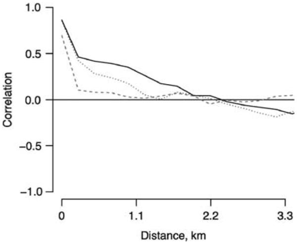
Correlogram of NO_x concentrations and model residuals.

We observed significantly better predictions of local pollution variation in our subset of lower-pollution (outside the LA basin, R² = 77%) communities than in our higherpollution (in-basin, R² = 72%) communities (Table 6). An increase of one IQR of CALINE4 TRP from freeways was associated with an 20.9% increase in NO_x in communities outside the LA basin, compared with an 14.1% increase for those within the LA basin. This difference in the relative impact of freeways was even larger for NO and NO₂. Similar findings were observed from a fixed-effects-only model (Supplementary Table B online). As shown in Table 6, the spatial random effects provided a greater improvement over a fixed-effects-only model for the in-basin communities than the out-of-basin communities, based on magnitude of the LRT statistics. This suggests that there are more un-modeled factors that impact local air quality in the LA basin, which is consistent with the general complexity and multitude of polluting sources in an urban area.

Table 6.

Percent change in pollutant level per increase of one interquartile range in the indicated predictor stratified by whether the communities are in or out of the Los Angeles basin.

Predictor variable	NO2		NO		NOX
	In basin	Out of basin	In basin	Out of basin	In basin	Out of basin
	% Change	% Change	% Change	% Change	% Change	% Change
CALINE-modeled TRP (freeway)	8.6****	16.3****	19.8****	31.1****	14.1****	20.9****
CALINE-modeled TRP (non-freeway)	3.9****	11.8****	14.1****	25.4****	10.4****	15.6****
Distance to nearest freeway	−0.6	1.2	−1.1	−0.1	−1.6	−1.9
Squared distance to nearest freeway	−0.3	0.4	0.9	0.3	0.5	−0.1
Distance to nearest non-freeway major road	−0.7	−2.7***	−2.6**	−2.4**	−1.1*	−2.9****
Non-freeway traffic volume within a 300m buffer	1.5****	−0.5	1.2	−6.3**	1.0*	−2.0
Population within a 300m buffer	1.2****	1.3	3.2****	−1.0	2.3	1.2
Neighborhood elevation relative to the community	−2.5****	−9.5****	−4.3****	−8.2****	−1.8***	−10.5****
LRT fixed versus spatial model	229.9****	38.2	248.8	32.7****	350.8****	35.5****
10-fold cross-validation R2	69%	72%	60%	72%	70%	76%

In-basin includes 658 sampling locations in eight communities within the Los Angeles basin. Out of basin includes 284 sampling locations in four communities outside the LA basin (see Table 1 for the specific communities). See Table 4 for the IQRs of the predicted variables.

^*P<0.1;

^**P<0.05;

^***P<0.005;

^****P<0.0005.

We used this model to predict the cumulative effect of living near a busy road on local levels of NO₂ (Figure 4), NO (Figure 5), and NO_x (Figure 6). For example, in an LA basin community with mean NO level of 26.0 p.p.b., our model predicts an average NO level of 18.5 p.p.b. for those living at least 1,500m from a freeway, and 26.2 p.p.b. (an increase of 7.6 p.p.b. and relative increase of 41.3%) for those living within 250m of a freeway (Figure 5). In a community outside the LA basin, our model predicts an average NO level of 5.1 p.p.b. at least 1,500m from a freeway and 8.9 p.p.b. (increase of 3.8 p.p.b. and relative increase of 75%) within 250m of a freeway. The absolute increase in out-of-basin communities is smaller, but given the lower average pollution levels in these more rural areas, the relative impact of freeways on exposure concentrations is larger than in the LA basin. These gradients in NO levels were of similar magnitude comparing distances 4300m to <75m from non-freeway major roads. Similar declines in predicted levels of NO₂ and NO_x were observed with increasing distance to roads.

Figure 4.

Predicted concentrations of NO₂ based on proximity to a freeway (FWY) or non-freeway (NFWY) major road. Vertical bars indicate the upper bound of the 95% confidence limit for each prediction. Results are shown for two types of communities: (a) within the LA basin with overall mean NO₂ level 25.3 p.p.b. and (b) outside the LA basin with overall mean 9.5 p.p.b.

Figure 5.

Predicted concentrations of NO based on proximity to a freeway (FWY) or non-freeway (NFWY) major road. Vertical bars indicate the upper bound of the 95% confidence limit for each prediction. Results are shown for two types of communities: (a) within the LA basin with overall mean NO level 26.0 p.p.b. and (b) outside the LA basin with overall mean 7.9 p.p.b.

Figure 6.

Predicted concentrations of NO_x based on proximity to a freeway (FWY) or non-freeway (NFWY) major road. Vertical bars indicate the upper bound of the 95% confidence limit for each prediction. Results are shown for two types of communities: (a) within the LA basin with overall mean NO_x level 57.3 p.p.b. and (b) outside the LA basin with overall mean 17.5 p.p.b.

Discussion

This study is unique in the emerging traffic-related exposure modeling literature because of the large number of measurements recorded from multiple communities. These provided an opportunity to examine how models performed in large and small urban locations and to evaluate the transferability of exposure models to locations where measurements were not made. We demonstrated that intra-community air quality can vary substantially and that in both large and small urban areas, traffic on busy roadways is the major determinant of this variation. We also observed significant contributions of population density and elevation on local air quality, but no impact of land-use categories. Inclusion of dispersionmodeled near-road pollution improved the model and was an influential determinant of concentrations of nitrogen oxides at our monitoring locations. Nevertheless, a model with widely available variables (roadway locations, traffic density, elevation, population density) can be used to build a good prediction of local air quality in the absence of dispersion model estimates. Furthermore, detailed land-use data, which are more difficult to obtain and are not uniformly collected across geographical regions, may not be necessary.

Our results suggest that the associations between local, near-road air quality, and traffic depend on the regional air quality. Specifically, we found that major roads and vehicular traffic have a larger relative impact in communities with lower average pollution than in more highly polluted communities. This indicates that in a low-pollution area, a major road represents the single largest source of pollution, and thus proximity to that road is the primary determinant of local variation in air quality. In a high-pollution area, on the other hand, there are likely to be many contributors to air quality other than major roads, including both point sources and transport from upwind sources. Spatial analysis of residuals from our models supports this conjecture, showing greater degree of spatial correlation in the residuals in our large urban compared with small urban communities. Although the relative contribution of major roads is less in a highpollution community, the absolute increase in pollution with closer proximity to a busy road is slightly greater than in a lower-pollution community (Figures 3–5). This is likely due to the fact that traffic volumes on busy roads are typically greater in a large urban than a small urban area.

Dispersion-modeled TRP based on CALINE4 was the best single predictor of measured pollutant levels. However, we found that simple distance to a freeway was still an important predictor of local pollutant levels in an urban area, even after adjusting for modeled TRP from a freeway. This may suggest that the CALINE4 dispersion model for estimating TRP does not completely capture the impact of a busy road on local pollutant levels. Alternatively, compared with a less-polluted area, an urban community may be more likely to have significant determinants of local air quality that are near busy roads such as shopping centers or other point sources. Thus, our observed associations with distance to roads in an urban area may simply be a surrogate for other sources that are not being captured by the CALINE4 dispersion model. Studies that have compared predicted pollution concentrations obtained by land-use regression to those obtained through dispersion modeling, generally have not shown dispersion models to perform better, but differences in models and in data used to develop the regressions make cross-study comparisons difficult (Briggs et al., 2000; Cyrys et al., 2005; Hoek et al., 2008; Marshall et al., 2008).

The predictions generated from our model demonstrated that residential distance to freeways and other major roads has a substantial impact on individual exposures to ambient NO, NO₂, and NO_x. This has implications for urban landuse policies, as proximity to sources of significant trafficrelated pollution (e.g., freeways and other busy roadways) has repeatedly been shown to be associated with elevated exposure (Roorda-Knape et al., 1998; Zhu et al., 2002, 2006; Zhou and Levy, 2007) and negative health outcomes (Edwards et al., 1994; Brunekreef et al., 1997; Hirsch et al., 1999; Venn et al., 2000, 2001; Brauer et al., 2002; Delfino, 2002; Nicolai et al., 2003; Kim et al., 2004; Zmirou et al., 2004; Gauderman et al., 2005, 2007; McConnell et al., 2006). Future placement of facilities and areas where people congregate (such as parks, schools, day care centers, and low-cost housing) should factor these findings into consideration.

Our models also have implications for studies of the health effects of traffic exposures. Traffic proximity measures have proven to be useful exposure indicators associated with a variety of health outcomes. However, health associations with traffic proximity have not been consistent across studies (Health Effects Institute, Special Report (2010)), and misclassification of exposure to the TRP mixture by simple proximity measures is one possible reason. Our models demonstrate that significantly better predictions of TRP exposure can be obtained by considering multiple factors simultaneously. These factors should not only include multiple indicators of traffic proximity and meteorology, but also non-traffic factors such as local elevation that can affect pollution dispersion. The use of improved estimates of traffic-related pollution exposure should result in increased power to detect health effects and more precise estimates of effect due to reduced measurement error.

The 10-fold cross-validation R² values of 0.63 (NO), 0.71 (NO₂) and 0.71 (NO_x) compares well with other land-use regression studies also based largely on traffic metrics, including a large study of NO₂ exposure at over 1,000 locations covering much of Connecticut (R² = 0.67; Skene et al., 2010) and a range of validation R² values from 0.49 to 0.78 across studies reported in a recent review (Hoek et al., 2008). Our leave-one-community out cross-validation based on 12 communities resulted in quite similar R² values (0.60 to 0.71), suggesting that the model may be transferable to other communities. This is considerably more promising than results from a limited number of other studies examining transferability of models in North America and Europe, which generally found that R² of models were considerably worse when transferred to other communities (Poplawski et al., 2008; Vienneau et al., 2010; Allen et al., 2011). However, the spatial scale of these studies was generally larger and the number of communities considerably smaller. The conditions under which models can be transferred between communities are an important issue, particularly since regional air pollution varies widely across the US. We noted differences in our estimates depending on whether communities were in or out of the LA basin. This gives evidence that regional differences in pollution mixtures influence near-roadway concentrations of nitrogen oxides, and thus accounting for these differences is an important consideration for transferring models such as those presented here to other areas.

Our findings and those of other investigators who have demonstrated intra-community variation in air quality may be important for the setting of national ambient air quality standards (NAAQS) by the US E_nvironmental Protection Agency (USEPA, 2010). A key component of the standard setting process for any of the criteria pollutants is the estimation of population risk for a variety of health effects (pre-mature death, lung function deficits, adverse symptoms, and so on). These risk calculations are typically computed using air quality information from fixed central site monitors in communities across the country, with particular attention given to those areas having pollutant levels that exceed some threshold. However, fixed-site central monitors are typically placed away from busy roads and other point sources in an attempt to capture general regional air quality. In southern California and elsewhere across the United States, many homes and schools are close to freeways or other major roadways and as a result are likely exposed to higher levels of NO₂ (and other traffic-related pollutants) than what is recorded at the closest central monitoring site. In the process of setting future national standards, consideration of intracommunity variation air quality should improve estimates of actual population exposures, and in turn yield more accurate estimates of population risks. In fact, the 2010 NO₂ NAAQS seeks to directly address this issue by establishing a monitoring network for NO₂ compliance near roadways.

We used diffusion-based passive samplers as a cost-efficient approach to obtain air quality information at over 900 sites spanning our 12 study communities. There may be other traffic-related pollutants (e.g., ultrafine PM, elemental carbon, benzene, and so on) that also vary locally and are more important determinants of health outcomes. The CHS is currently conducting an extensive air monitoring study aimed at measuring local levels of PM, including both mass and chemical constituents. That data, in conjunction with the NO_x data from this study, will provide a more complete picture of how air quality varies locally and regionally, allowing for further investigation of how different mixtures may influence traffic-related pollution. Furthermore, with a wider range of pollutant measurements, a more thorough examination of which specific pollutants most affect children’s health can be conducted.

We also note that while the primary focus of this study was to investigate factors that relate to variability in air quality at a local scale, the implication of utilizing deviations (i.e., subtracting community-wide means from the measurements) is that baseline differences between the 12 communities studied cannot be directly explained. Models that harness averaged information would allow for such analyses, should variability resulting from community differences in land use or traffic indicators be of research interest.

We have demonstrated that in southern California, there is substantial variation in local, intra-community air quality in both large and small urban environments and that proximity to busy roads is a major determinant of that variation. This finding has potential ramifications for urban land-use policy, calculation of pollution-related health risks, and the setting of national air quality standards. Strategies for reducing population exposure to traffic-related pollutants should continue to be a priority for local, state, and national agencies.

References

- Allen RW, Amram O, Wheeler AJ, Brauer M. The transferability of NO and NO2 land use regression models between cities and pollutants. Atmos Environ. 2011;45(2):369–378. [Google Scholar]
- Beckerman B, Jerrett M, Brook JR, Verma DK, Arain MA, Finkelstein MM. Correlation of nitrogen dioxide with other traffic pollutants near a major expressway. Atmos Environ. 2008;42:275–290. [Google Scholar]
- Benson P. CALINE4–A Dispersion Model for Predicting Air Pollutant Concentrations Near Roadways. California Department of Transportation; Sacramento, CA: 1989. Report No. FHWA/CA/TL-84/15. [Google Scholar]
- Brauer M, Hoek G, Van Vliet P, Meliefste K, Fischer PH, Wijga A, et al. Air pollution from traffic and the development of respiratory infections and asthmatic and allergic symptoms in children. Am J Respir Crit CareMed. 2002;166(8):1092–1098. doi: 10.1164/rccm.200108-007OC. [DOI] [PubMed] [Google Scholar]
- Briggs D, de Hoogh C, Gulliver J, Elliotta P, Kingham S, Smallboned K. A regression-based method for mapping traffic-related air pollution: application and testing in four contrasting urban environments. Sci Total Environ. 2000;253(1-3):151–167. doi: 10.1016/s0048-9697(00)00429-0. [DOI] [PubMed] [Google Scholar]
- Brunekreef B, Janssen N, de Hartog J, Harssema H, Knape M, van Vliet P. Air pollution from truck traffic and lung function in children living near motorways. Am J Epidemiol. 1997;8:298–303. doi: 10.1097/00001648-199705000-00012. [DOI] [PubMed] [Google Scholar]
- California Air Resources Board . Calculating Emission Inventories For Vehicles In California. CARB; Sacramento, CA: 2007. User’s Guide to EMFAC2007, Version 2.30. [Google Scholar]
- Caltrans . Caltrans 2007 California Motor Vehicle Stock, Travel and Fuel Forecast. California Department of Transportation; Sacramento, CA: May, 2008. 2008. [Google Scholar]
- Chinkin LR, Main HH, Roberts PT. Weekday/weekend Ozone Observations In The South Coast Air Basin Volume III: Analysis Of Summer 2000 Field Measurements And Supporting Data Final report STI-999670-2124-FR. Sonoma Technology, Inc.; Petaluma, CA: 2002. [Google Scholar]
- Cyrys J, Hochadel M, Gehring U, Hoek G, Diegmann V, Brunekreef B, et al. GIS-based estimation of exposure to particulate matter and NO2 in an urban area: stochastic versus dispersion modeling. Environ Health Perspect. 2005;113(8):987–992. doi: 10.1289/ehp.7662. [DOI] [PMC free article] [PubMed] [Google Scholar]
- Delfino RJ. Epidemiologic evidence for asthma and exposure to air toxics: linkages between occupational, indoor, and community air pollution research. Environ Health Perspect. 2002;110(Suppl 4):573–589. doi: 10.1289/ehp.02110s4573. [DOI] [PMC free article] [PubMed] [Google Scholar]
- Dijkema MBA, Gehring U, van Strien RT, van der Zee SC, Fischer P, Hoek G, et al. A comparison of different approaches to estimate small scale spatial variation in outdoor NO2 concentrations. Environ Health Perspect. 2010;119(5):670–675. doi: 10.1289/ehp.0901818. [DOI] [PMC free article] [PubMed] [Google Scholar]
- Dockery D, Cunningham J, Damokosh A, Neas L, Spengler J, Koutrakis P, et al. Health effects of acid aerosols on North American children: respiratory symptoms. Environ Health Perspect. 1996;104:500–505. doi: 10.1289/ehp.96104500. [DOI] [PMC free article] [PubMed] [Google Scholar]
- Dockery DW, Pope CA, 3rd, Xu X, Spengler JD, Ware JH, Fay ME, et al. An association between air pollution and mortality in six U.S. cities. N Engl J Med. 1993;329(24):1753–1759. doi: 10.1056/NEJM199312093292401. [DOI] [PubMed] [Google Scholar]
- Edwards J, Walters S, Griffiths RK. Hospital admissions for asthma in preschool children: relationship to major roads in Birmingham, United Kingdom. Arch Environ Health. 1994;49(4):223–227. doi: 10.1080/00039896.1994.9937471. [DOI] [PubMed] [Google Scholar]
- Gauderman WJ, Avol E, Gilliland F, Vora H, Thomas D, Berhane K, et al. The effect of air pollution on lung development from 10 to 18 years of age. N Engl JMed. 2004;351(11):1057–1067. doi: 10.1056/NEJMoa040610. [DOI] [PubMed] [Google Scholar]
- Gauderman WJ, Avol E, Lurmann F, Kuenzli N, Gilliland F, Peters J, et al. Childhood asthma and exposure to traffic and nitrogen dioxide. Epidemiology. 2005;16(6):737–743. doi: 10.1097/01.ede.0000181308.51440.75. [DOI] [PubMed] [Google Scholar]
- Gauderman WJ, Vora H, McConnell R, Berhane K, Gilliland F, Thomas D, et al. Effect of exposure to traffic on lung development from 10 to 18 years of age: a cohort study. Lancet. 2007;369(9561):571–577. doi: 10.1016/S0140-6736(07)60037-3. [DOI] [PubMed] [Google Scholar]
- Gilbert NL, Woodhouse S, Stieb DM, Brook JR. Ambient nitrogen dioxide and distance from a major highway. Sci Total Environ. 2003;312:43–46. doi: 10.1016/S0048-9697(03)00228-6. [DOI] [PubMed] [Google Scholar]
- Gotschi T, Sunyer J, Chinn S, de Marco R, Forsberg B, Gauderman JW, et al. Air pollution and lung function in the European Community Respiratory Health Survey. Int J Epidemiol. 2008;37(6):1349–1358. doi: 10.1093/ije/dyn136. [DOI] [PMC free article] [PubMed] [Google Scholar]
- Hart JE, Yanosky JD, Puett RC, Ryan L, Dockery DW, Smith TJ, et al. Spatial modeling of PM10 and NO2 in the continental United States, 1985–2000. Environ Health Perspect. 2009;117:1690–1696. doi: 10.1289/ehp.0900840. [DOI] [PMC free article] [PubMed] [Google Scholar]
- Health Effects Institute, Special Report . Traffic-Related Air Pollution: A Critical Review of the Literature on Emissions, Exposure, and Health Effects. HEI; Boston,MA: 2010. [Google Scholar]
- Hirsch T, Weiland SK, von Mutius E, Safeca AF, Grafe H, Csaplovics E, et al. Inner city air pollution and respiratory health and atopy in children. Eur Respir J. 1999;14(3):669–677. doi: 10.1034/j.1399-3003.1999.14c29.x. [DOI] [PubMed] [Google Scholar]
- Hoek G, Beelen R, de Hoogh K, Vienneau D, Gulliver J, Fischer P, et al. A review of land-use regression models to assess spatial variation of outdoor air pollution. Atmos Environ. 2008;42:7561–7578. [Google Scholar]
- Kan H, Heiss G, Rose KM, Whitsel EA, Lurmann F, London SJ. Prospective analysis of traffic exposure as a risk factor for incident coronary heart disease: the Atherosclerosis Risk in Communities (ARIC) study. Environ Health Perspect. 2008;116:1463–1468. doi: 10.1289/ehp.11290. [DOI] [PMC free article] [PubMed] [Google Scholar]
- Kim J, Smorodinsky S, Lipsett M, Singer BC, Hodgson AT, Ostro B. Traffic-related air pollution near busy roads: the East Bay Children’s Respiratory Health Study. Am J Resp Crit Care Med. 2004;170:520–526. doi: 10.1164/rccm.200403-281OC. [DOI] [PubMed] [Google Scholar]
- Koutrakis P, Wolfson JM, Bunyaviroch A, Froehlich SA. Passive Ozone Sampler Based On A Reaction with Nitrite. Health Effects Institute; Boston, MA: 1994. pp. 19–47. [PubMed] [Google Scholar]
- Marshall J, Nethery E, Brauer M. Within-urban variability in ambient air pollution: comparison of estimation methods. Atmos Environ. 2008;42:1359–1369. [Google Scholar]
- McConnell R, Berhane K, Gilliland F, London SJ, Vora H, Avol E, et al. Air pollution and bronchitic symptoms in Southern California children with asthma. Environ Health Perspect. 1999;107(9):757–760. doi: 10.1289/ehp.99107757. [DOI] [PMC free article] [PubMed] [Google Scholar]
- McConnell R, Berhane K, Gilliland F, Molitor J, Thomas D, Lurmann F, et al. Prospective study of air pollution and bronchitic symptoms in children with asthma. Am J Respir Crit Care Med. 2003;168(7):790–797. doi: 10.1164/rccm.200304-466OC. [DOI] [PubMed] [Google Scholar]
- McConnell R, Berhane K, Lurmann F, Molitor J, Gauderman W, Avol E, et al. Traffic and asthma prevalence in children. Am J Respir Crit CareMed. 2002;165:A492. [Google Scholar]
- McConnell R, Berhane K, Yao L, Jerrett M, Lurmann F, Gilliland F, et al. Traffic, susceptibility, and childhood asthma. Environ Health Perspect. 2006;114(5):766–772. doi: 10.1289/ehp.8594. [DOI] [PMC free article] [PubMed] [Google Scholar]
- Nicolai T, Carr D, Weiland SK, Duhme H, von Ehrenstein O, Wagner C, et al. Urban traffic and pollutant exposure related to respiratory outcomes and atopy in a large sample of children. Eur Respir J. 2003;21(6):956–963. doi: 10.1183/09031936.03.00041103a. [DOI] [PubMed] [Google Scholar]
- Peters A. Air quality and cardiovascular health: smoke and pollution matter. Circulation. 2009;120(11):924–927. doi: 10.1161/CIRCULATIONAHA.109.895524. [DOI] [PubMed] [Google Scholar]
- Peters JM, Avol E, Navidi W, London SJ, Gauderman WJ, Lurmann F, et al. A study of twelve Southern California communities with differing levels and types of air pollution. I. Prevalence of respiratory morbidity. Am J Respir Crit Care Med. 1999;159(3):760–767. doi: 10.1164/ajrccm.159.3.9804143. [DOI] [PubMed] [Google Scholar]
- Poplawski K, Gould T, Setton E, Allen R, Su J, Larson T, et al. Intercity transferability of land use regression models for estimating ambient concentrations of nitrogen dioxide. J Expos Sci Environ Epidemiol. 2008;19:107–117. doi: 10.1038/jes.2008.15. [DOI] [PubMed] [Google Scholar]
- Roorda-Knape MC, Janssen NAH, de Hartog JJ, Van Vliet PHN, Harssema H, Brunekreef B. Air pollution from traffic in city districtc near major motorways. Atmos Environ. 1998;32(11):1921–1930. [Google Scholar]
- Skene KJ, Gent JF, McKay LA, Belanger K, Leaderer BP, Holford TR. Modeling effects of traffic and landscape characteristics on ambient nitrogen dioxide levels in Connecticut. Atmos Environ. 2010;44(39):5156–5164. doi: 10.1016/j.atmosenv.2010.08.058. [DOI] [PMC free article] [PubMed] [Google Scholar]
- US Environmental Protection Agency . Strengthened National Standards for Nitrogen Dioxide. USEPA; Research Triangle Park, NC: 2010. http://www.epa.gov/airquality/nitrogenoxides/actions.html. [Google Scholar]
- Venn A, Lewis S, Cooper M, Hubbard R, Hill I, Boddy R, et al. Local road traffic activity and the prevalence, severity, and persistence of wheeze in school children: combined cross sectional and longitudinal study. Occup Environ Med. 2000;57(3):152–158. doi: 10.1136/oem.57.3.152. [DOI] [PMC free article] [PubMed] [Google Scholar]
- Venn AJ, Lewis SA, Cooper M, Hubbard R, Britton J. Living near a main road and the risk of wheezing illness in children. Am J Respir Crit Care Med. 2001;164(12):2177–2180. doi: 10.1164/ajrccm.164.12.2106126. [DOI] [PubMed] [Google Scholar]
- Vienneau D, de Hoogh K, Beelen R, Fischer P, Hoek G, Briggs D. Comparison of land-use regression models between Great Britain and the Netherlands. Atmos Environ. 2010;44(5):688–696. [Google Scholar]
- Waller L, Gotway C. Applied Spatial Statistics for Public Health Data. Wiley; Hoboken, NJ: 2004. [Google Scholar]
- Wu J, Funk T, Lurmann F, Winer AM. Improving spatial accuracy of roadway networks and geocoded addresses. Trans GIS. 2005;9(4):585–601. [Google Scholar]
- Zhou Y, Levy JI. Factors influencing the spatial extent of mobile source air pollution impacts: A meta-analysis. BMC Public Health. 2007;7:89. doi: 10.1186/1471-2458-7-89. [DOI] [PMC free article] [PubMed] [Google Scholar]
- Zhu Y, Hinds WC, Kim S, Sioutas C. Concentration and size distribution of ultrafine particles near a major highway. J Air Waste Manag Assoc. 2002;52(9):1032–1042. doi: 10.1080/10473289.2002.10470842. [DOI] [PubMed] [Google Scholar]
- Zhu Y, Kuhn T, Mayo P, Hinds WC. Comparison of daytime and nighttime concentration profiles and size distributions of ultrafine particles near a major highway. Environ Sci Technol. 2006;40:2531–2536. doi: 10.1021/es0516514. [DOI] [PubMed] [Google Scholar]
- Zmirou D, Gauvin S, Pin I, Momas I, Sahraoui F, Just J, et al. Traffic related air pollution and incidence of childhood asthma: results of the Vesta case-control study. J Epidemiol Community Health. 2004;58:18–23. doi: 10.1136/jech.58.1.18. [DOI] [PMC free article] [PubMed] [Google Scholar]
Associated Data
This section collects any data citations, data availability statements, or supplementary materials included in this article.