Abstract
We proposed a maximum a posterior (MAP) framework for incorporating information from co-registered anatomical images into PET image reconstruction through a novel anato-functional joint prior. The characteristic of the utilized hyperbolic potential function is determinate by the voxel intensity differences within the anatomical image, while the penalization is computed based on voxel intensity differences in reconstructed PET images. Using realistic simulated 18FDG PET scan data, we optimized the performance of the proposed MAP reconstruction with the joint prior (JP-MAP), and compared its performance with conventional 3D MLEM and 3D MAP reconstructions. The proposed JP-MAP reconstruction algorithm resulted in quantitatively enhanced reconstructed images, as demonstrated in extensive FDG PET simulation study. The proposed method was also tested on a 20 min Florbetapir patient study performed on the high-resolution research tomograph. It was shown to outperform conventional methods in visual as well as quantitative accuracy assessment (in terms of regional noise versus activity value performance). The JP-MAP method was also compared with another MR-guided MAP reconstruction method, utilizing the Bowsher prior, and was seen to result in some quantitative enhancements especially in the case of MR-PET mis-registrations, and a definitive improvement in computational performance.
1. Introduction
Positron emission tomography (PET) is a powerful molecular imaging modality enabling quantitative measurements of physiological and biochemical process in vivo. However, the quantitative accuracy of PET imaging is limited by several factors including the intrinsic resolution of the imaging system and inherently noisy data (Rahmim and Zaidi, 2008). Comparing to analytical reconstruction (e.g. filtered backprojection), statistical reconstruction methods, such as maximum likelihood (ML) or maximum a posterior (MAP), can incorporate noise statistics and system matrix modeling (Leahy and Qi, 2000). ML estimates often exhibit high noise propagations, while Bayesian or MAP methods attempt to stabilize the image estimates through incorporation of prior models. The commonly invoked quadratic prior often leads to blurring of the edges (Geman and Geman, 1984). Non-quadratic priors, such as the Green (Green, 1990), Huber (Mumcuoglu et al., 1996) and hyperbolic (Charbonnier et al., 1997) priors, can enhance tolerance for edges but the results can be sensitive to the value of the hyper-parameter that controls the shape of the potential function. Nevertheless, a drawback of these non-quadratic edge-preserving priors is that voxel intensity differences may not be robust and reliable in distinguishing real edges from noisy fluctuation when an image is noisy.
An alternative approach seeks to preserve edges via incorporation of anatomical information (Bai et al., 2013). Some approaches seek to control regularization (e.g. quadratic penalty or prior) by preventing the smoothing across anatomical boundaries to avoid activity spillover between distinct regions (Fessler et al., 1992; Alessio et al., 2006). A related approach is to control regularization weights based on the labels of the two voxels via a segmentation process (Sastry and Carson, 1997; Comtat et al., 2002). Others seek to encourage a homogeneous distribution of tracers within each anatomical region (Lipinski et al., 1997). More flexible techniques incorporating differences between anatomical and functional segmentation (e.g. hot spots in brain stimulation studies or cold spots in arterial stenosis or occlusions) were also proposed by Bowsher et al (1996) and Rangarajan et al (2000). In any case, these techniques still rely on the explicit boundary or regional information derived from anatomical images by segmentation or edge detection.
Bowsher et al (2004) proposed an anatomical prior avoiding need for segmented anatomical information. This prior (referred to as the Bowsher prior) encourages smoothing over an anatomy-dependent neighborhood, defined by selecting a set of most similar neighbors in the anatomical image (Vunckx et al., 2012). As an extension, Bousse et al (2010) presented a generalization of the Bowsher prior, taking into account each neighbor with a substitute weight. Furthermore, Kazantsev et al (2011) presented a non-local algorithm for the weights estimation, which was included into the modified Bowsher prior in order to improve the robustness of the method to non-correlated information between activity and anatomy. Chun et al (2012) proposed a non-local means methods to incorporate side information in SPECT/CT reconstruction, while Nguyen and Lee (2013) proposed a new approach to incorporating prior anatomical information within PET reconstruction using the non-local regularization method, designed to selectively take into account the anatomical information only when it is reliable. Overall, all these methods try to modify the weight of the potential function (commonly quadratic function) based on the anatomical information rather than the PET image itself.
Other recent work has tended to apply no segmentation of the anatomy but involve information–based similarity measures between the anatomical and reconstructed PET images. Sophisticated information-based similarity measure priors have as a result appeared in the literature (Nuyts, 2007; Tang and Rahmim, 2009a, b; Somayajula et al., 2011; Lu et al., 2011; Vunckx et al., 2012; Van de Sompel and Brady, 2012). Challenges with these information-theoretic priors include the non-convexity of the priors, the sensitivity to the choice of the specific parameters, and the choice of the initial image.
The present work, by contrast, investigates the use of a straightforward convex hyperbolic potential function employing non-segmented anatomical information to enhance the PET image reconstruction. The characteristic of the potential function is determined by the voxel intensity differences in the anatomical image, while the penalization is computed based on voxel intensity differences in the PET images. As we shall also demonstrate, our approach results in a framework that is robust to the choice of parameters. We have designed and investigated a one-step-late (OSL) maximum a posteriori (MAP) algorithm incorporating the anatomical information via the joint prior. We optimized the regularization parameter as well as the parameter characterizing the reconstruction algorithm using realistic HRRT brain imaging studies. The performance of the proposed techniques was evaluated in terms of regional and overall NSD (noise) versus Bias. The quality of images reconstructed from the proposed algorithm was in particular compared with that of images from conventional ML and MAP reconstruction. Furthermore, the proposed techniques were also evaluated with different MR image noise levels and the additional effect of PET-MR mis-registration, as considered in (Gravel et al., 2013). Parts of this work were presented at the 2014 International Symposium of Biomedical Imaging (Lu et al., 2014) and Society of Nuclear Medicine and Molecular imaging 2014 Annual Meeting (Lu et al., 2014).
2. Methods
2.1. MAP PET image reconstruction
Let f={fj} denote the unknown emission distribution. The PET data g={gi}, modeled as a collection of independent Poisson random variables with expectation ḡ={ḡi}, can be related to f through an affine transform:
| (1) |
where P ∈ Rni×nj is the system matrix with element denoting the probability of a positron emitted from voxel j resulting in a coincidence at the i th detector pairs, and r ∈ Rni accounts for the scattered and random events, and ni and nj denote the total number of detector pairs and voxels, respectively.
According to the measurement model, the log-likelihood function of the measured data is given by
| (2) |
where g and f denote the measured sinograms and the unknown emission distributions, respectively.
Maximum likelihood (ML) estimation attempts to maximize L(g|f) with respect to f. However, ML estimation will produce increasing noise levels with increasing iterations. A powerful method to circumvent daunting noise levels is to utilize Bayesian theory to maximize the posterior probability that includes prior image information. The prior information can be specified by a probability density on f and subsequently combined with the information contained in g to produce an estimation of the unknown image. Commonly, the prior is modeled to follows a Gibbs distribution (Geman and Geman, 1984):
| (3) |
where U(f) is the energy function and β is a regularization parameter that controls the tradeoff between resolution and noise. Combining the likelihood function and the image prior, MAP estimation of f is given by
| (4) |
Based on equations (2) and (4), we then invoke the one-step-late (OSL) approach for an iterative update to the MAP estimate (Green, 1990):
| (5) |
where the new estimate of voxel j is updated from the old estimate. A single bin i of the measured sinogram g is represented by gi, and pij represents an element of the system matrix P. The performance of the MAP reconstruction strongly depends on the construction of the prior U(f) and the regularization parameter β, which we will elaborate upon in section 2.3 and 4.1.1, respectively.
2.2. Generation of the prior model
2.2.1. Conventional priors
The prior energy function U(f) in (4) is commonly computed via a weighted sum of potential functions v of the differences between voxels in the local neighborhood Nj:
| (6) |
where wkj is the weight of a given pixel k in the neighborhood of pixel j. For 3D image reconstructions, a neighborhood with 18 neighbors was selected. The weight wkj is set to 1 if k and j are orthogonal nearest neighbors, to for diagonal neighbors and to 0 otherwise. Generally, different choices of potential function v lead to different priors. The prior becomes a quadratic prior when the potential function v takes the form v(t) = t2. In this paper, we focus on the hyperbolic potential function:
| (7) |
where δ is a free parameter to be optimized (Charbonnier et al., 1997). The ordinary derivative of this potential function is given by
| (8) |
To illustrate the characteristic of the potential function, figure 1 plots the partial derivative of this potential function for different value of δ. Note that we plot rather than , in order to normalize the limit value to unity as t increases. The potential function is always an edge-preserving function.
Figure 1.
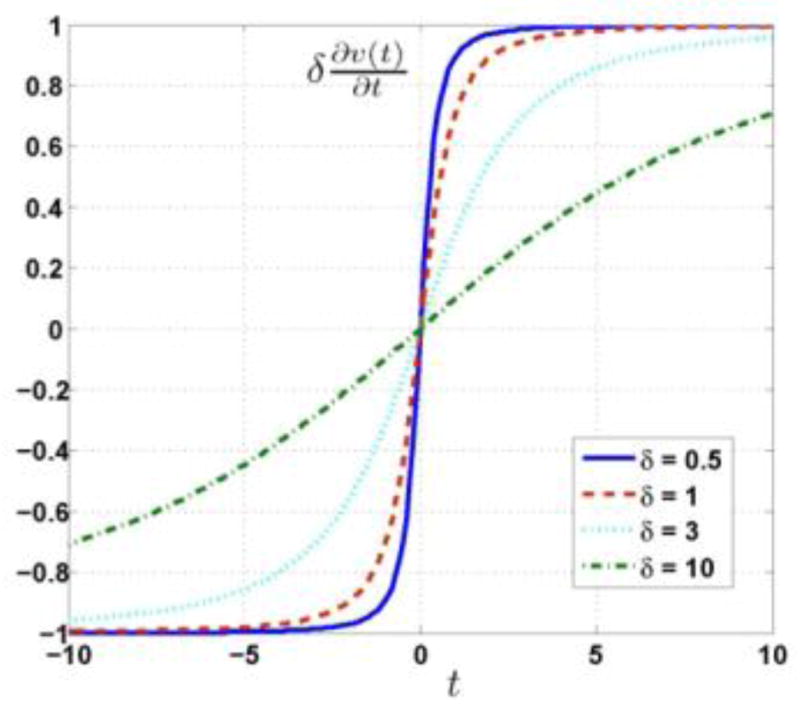
Plots of partial derivative of hyperbolic potential function for different values of δ.
2.2.2. The proposed joint potential function
The prior term can be used to incorporate a priori information about the PET image. We utilize information that can be available through co-registered anatomical images. Assume that the PET image f and the anatomical image a are very well registered. If neighboring voxel values in the anatomical image a are similar, the corresponding voxels in the PET image are more likely to belong to the same organ or region. Thus, we define a joint prior that includes both the anatomical and functional information:
| (9) |
where wkj is the weight of a given voxel k in the neighborhood of voxel j, as elaborated in section 2.2.1, and nj and Nj are defined as those in (6). The joint potential function is defined as
| (10) |
where Δfjk = fj − fk and Δajk = aj − ak, δ is defined as that in (7), and η is an adjustable parameter in the prior. The partial derivative of the joint potential function is analogous to a force that tries to reduce the difference between neighboring voxels in the PET image f, and
| (11) |
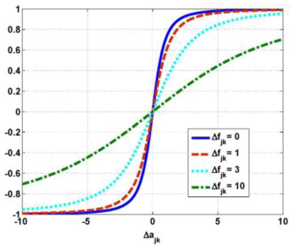
Figure 2 plots the derivative as a function of Δajk for some fixed Δfjk, where δ and η are 1. Note that the “force” increases more rapidly as a function of the difference Δajk in the anatomical image a when the difference Δfjk in the PET image f is smaller. Thus, small differences in the voxel values of neighboring pixels in the anatomical image a apply more “force” to smooth differences in the voxel values in the PET image f. Similarly, large difference in neighboring voxel values in the anatomical image a apply less “force” to smooth differences in the voxels in the PET image f. Thus, the derivative of joint potential function is adaptively modified based on the anatomical information.
Figure 2.
Plots of the derivative as a function of Δajk for some fixed Δfjk where δ and η are 1.
2.2.3. The Bowsher-Prior
The Bowsher-prior is a smoothing Markov prior operating on a position dependent neighborhood. The prior energy function U(f) has the similar form as equation (6):
| (12) |
where v is the potential function and Nj(a,B) is a subset of Nj (the neighborhood of j as defined in (6)) containing the B (number of neighbor) voxels k1,···,kB, which are fulfilling
| (13) |
In the original bowsher prior (Bowsher J E et al 2004), for voxel belonging to the cliques Nj(a,B), wkj are set to 1, while others are set to 0. At the same time, wkj could be a function of (aj−ak), as elaborated in the literature (Bousse et al 2010, Kazantsev et al 2011). In our study, the weight is adopted from the original bowsher prior and v takes the form v(t) = t2.
2.3. Parameter model
The performance of a MAP reconstruction algorithm strongly depends on the construction of the prior and the regularization parameter (β in (5)), which determines how much a role the prior plays in the reconstruction process. The construction of the single hyperbolic prior and joint prior model strongly depend on the parameter δ in (7, 10) and η in (10). In principle, δ and η may be different due to differences in the scale of the two images. In He et al (2011), the parameter δ and η as used in the cross tracer prior were set to equal values for dual-isotope myocardial perfusion SPECT imaging. This makes sense because the two images for dual tracer imaging should have similar scales. In our initial study, the δ and η were set to constant values and optimized independently of each other. However, we found that for each δ, a different optimal value β exists, which makes the optimization strategy more complicated for different η values. Here, we propose the following parameter model:
| (14) |
is the mean gradient value of the PET image at the n th iteration and α is a scale parameter. To balance the contributions of the functional image f and anatomical image a in the joint potential function, the parameter η can be set as:
| (15) |
where is the mean gradient value of the MR image at the n th iteration. Thus, we simplify the optimization strategy by focusing on a single parameter α.
3. Experimental design
3.1. Simulation study
3.1.1. MR simulation
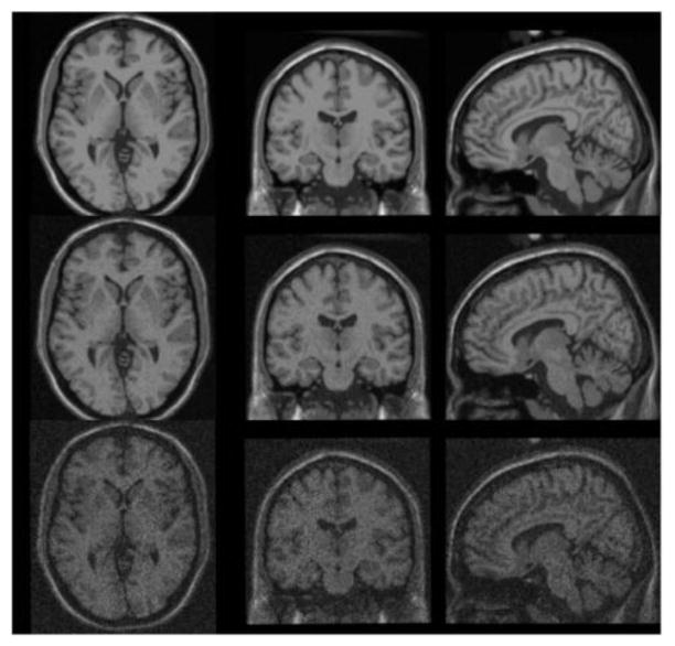
For realistic MR simulation, the simulated T1-weighted MR-image and the label image was derived from the BrainWeb database (Collins et al., 1998). The label image included 9 individual regions of the brain (cerebrospinal fluid (CSF), grey matter (GM), white matter (WM), fat, muscle, skin, skull, glial matter, connective tissue and background). The MR image has matrix dimensions of 256×256×207 and cubic voxel sizes of 1.219×1.219×1.219mm3. To evaluate the robustness in the presence of noise, the MR-image was simulated with noise level 3%, 9% and 15%, which corresponding to low, middle, and high noise level in realistic MR images respectively, as shown in figure 3. Furthermore, to evaluate the robustness in the presence of registration errors, the MR-images with different noise levels were applied a 3D rigid body motion to simulate the mis-registration. The 3D rigid body motion can be completely characterized by the set of 4×4 transformation matrices as described in (Mohy-ud-Din et al., 2011)
Figure 3.
(Top to bottom) The simulated brain MR-image with different noise levels of 3%, 9%, and 15%, respectively (from left to right corresponding to transaxial, coronal and sagittal slices).
| (16) |
SO(3) is the group of 3D rotational matrices with special properties, v is the translation matrix, and R is the rotation matrix. For brain imaging, the rotation angle with respect to the z direction is set to −1°, and translation is set to 2.0 mm with respect to x, y and z for a total distance of mm. This assumption was reasonable for PET brain imaging, as errors below 3 mm were reported for rigid registration of PET/MR brain images using state-of-the-art registration algorithms (Slomka and Baum, 2009).
3.1.2. PET simulation
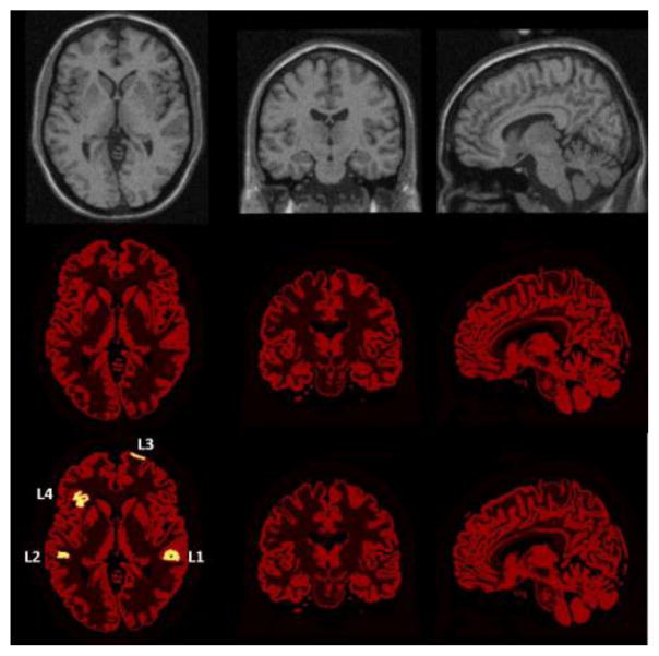
Taking into account known relative intensities in clinical 18F-FDG brain study, a brain PET activity distribution was created with each tissue class (in the label image) assigned an activity value: 12500Bq/ml in GM, 3125Bq/ml in WM, 0Bq/ml in air, CSF and bone, and 1000Bq/ml in all other tissue as shown in figure 4 (middle). The noisy MR-image (9% noise calculated relative to the brightest tissue) is shown in the figure 4 (top). The corresponding attenuation map was created with each tissue class (in the label image) assigned a realistic attenuation coefficient.
Figure 4.
(Top) The simulated brain MR-image, and the brain PET phantom (middle) without and (bottom) with lesions, from left to right corresponding to transaxial, coronal and sagittal slices. The lesions visible in the transaxial slices are labeled with L1, L2, L3 and L4.
To simulate the possibility that some subtle lesions are detected by PET but not picked up by MRI, a brain PET activity distribution with hyperactive gray matter lesions was created as shown in figure 4 (bottom). Four lesions, labeled with L1, L2, L3 and L4 in figure 4 (bottom), were created by distributing 4 spheres with a diameter of 20 mm over the grey matter, encompassing cortical and subcortical cerebral regions. The tracer uptake of the gray matter inside each sphere was increased by 100%, while the activity of other classes was unaffected. Consequently, the actual volume of the lesion was different in every lesion, and much smaller than the volume of the sphere. This represents a reasonable intermediary size for clinical lesions.
We performed realistic analytic simulations for the geometry of the high resolution research tomograph (HRRT) (Sossi et al., 2005), a dedicated-brain 3D-only acquisition system. The simulator forward-projects the image to generate the noise free projection data. Then the data was scaled and 30 noise realizations were generated utilizing Poisson noise on projections with clinically realistic counts (100M). Decay, normalization and attenuation effects were taken into account, and these effects were also incorporated within the reconstructions. Decay is computed based on the half-life of 18FDG, normalization is derived from the clinical HRRT scanner, and attenuation sinogram is obtained by projecting the brain attenuation map.
PET images were reconstructed from: (i) conventional 3D reconstruction (MLEM), (ii) conventional 3D MAP reconstruction with the single hyperbolic prior (SP-MAP), (iii) 3D MAP reconstruction with the bowsher prior (BP-MAP), and (iv) proposed 3D MAP reconstruction with the joint prior (JP-MAP). 10 iterations with 16 subsets were adapted for different reconstruction approaches, as elaborated in 4.1 and 4.2. All images were reconstructed with matrix dimensions of 256×256×207 and cubic voxel sizes of 1.219×1.219×1.219mm3.
3.1.3. Figures of Merit (FOMs)
To compare the images reconstructed from the different algorithms described in the previous subsection, the following quantitative evaluation criteria were considered.
The mean squared error (MSE) was defined as
| (17) |
where N is the number of voxels in the ROI, Xj denotes the reconstructed PET image value at a voxel j, and denotes the reference ground truth PET image value at a voxel j.
The normalized standard deviation (NSDROI) for each ROI was defined as
| (18) |
where N and j were defined as those in (17), and R is the number of noise realizations; denotes the r th reconstructed PET image value at a voxel j of the specified ROI, and represents the ensemble mean value of reconstructed PET image value at a voxel j. For a given ROI of known PET image value, the regional bias (BiasROI) was defined as
| (19) |
where and and were defined as those in (17) and (18) respectively.
To quantify the ability of a given reconstructed image to recover the contrast between the lesion and normal background areas, the contrast is defined as
| (20) |
where and are the average value from the background and lesion regions of the rth noise realization, respectively. The contrast recovery ratio (CRR) was calculated as the ratio between the contrast estimated from the reconstructed image and the true contrast in the phantom image. Overall FOMs: To quantify NSDoverall versus Biasoverall for the entire image (in order to allow an overall assessment of quantitative performance), NSDROI and BiasROI values for the ROIs were averaged, and weighted by the size (number of voxels N) for each ROI to estimate the overall NSD and Bias.
3.2. Application to patient study
We also considered application of the proposed method to subject data from the HRRT scanner. We modified the existing HRRT reconstruction code to enable both: (i) standard 3D reconstruction (MLEM), and (ii) proposed 3D MAP reconstruction with the joint prior (JP-MAP). In addition to correction for attenuation and normalization, corrections for random and scatter events were also performed, which were estimated using the singles rate method and the standard single scatter simulation, respectively, for the HRRT scanner (Rahmim et al., 2005).
[18F]Florbetapir (Amyvid) PET amyloid imaging is a diagnostic tool for patients with cognitive impairment who are being evaluated for Alzheimer’s Disease (AD) and other causes of cognitive decline (Yang et al., 2012). A 20-minute Florbetapir PET scan on a 50 year old male, with acquisition spanning 50 to 70 minutes was obtained. The MR image was fully registered with the initial reconstructed PET image. As in the simulation, up to 10 iterations (16 subsets each) for both aforementioned conventional and proposed approaches were generated.
Since the true activity values are not known, no analysis of bias was performed. Instead, we plotted ActivityROI versus NSDROI for a variety of ROIs, where NSDROI was defined as in (13). This would allow comparisons of noise performance given matched activity values.
4. Results
We evaluated the proposed MAP reconstruction (JP-MAP) algorithm in comparison with conventional 3D MLEM and MAP reconstruction algorithms with single hyperbolic prior (SP-MAP) and Bowsher prior (BP-AMP). The parameters in all algorithms were first optimized separately, and followed by quantitative comparison in terms of the ensemble noise versus bias (or contrast recovery ratio) performance over the 30 noise realizations.
4.1. Simulation study
4.1.1. Parameter Optimization
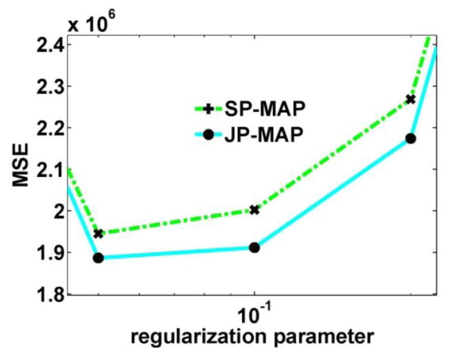
First, the effect of varying parameter δ vs. proposed parameter α was illustrated in Figure 5a vs. b, respectively. For the δ -values plotted in figure 5(a), when δ1/2 increased from 10 to 100, the corresponding optimized β increased from 0.02 to 0.5. For the α -value plotted in figure 5(b), when α increased from 0.001 to 1, the optimized β was 0.02. From figure 5(a) and (b), we can see that the proposed parameter model can achieve similarly low MSE values; however, interestingly, the selection is considerably robust to the particular chose of α values. Furthermore, upon closer inspection (Fig. 6) when using optimal α parameters (for SP-MAP and JP-MAP), it is seen that the JP-MAP framework results in improved quantitative performance compared to the SP-MAP framework.
Figure 5.
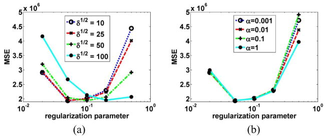
(a) Plots of MSE as a function of the regularization parameter for SP-MAP reconstructed images at 10 iterations (16 subsets) for different δ values. (b) Plots of MSE as a function of the regularization parameter for SP-MAP reconstructed images at 10 iterations (16 subsets) for different α values.
Figure 6.
Plots of MSE as a function of the regularization parameter for images from: (i) SP-MAP reconstruction using the proposed parameter model δn, and (ii) JP-MAP reconstruction using the proposed parameter model δn and ηn, at 10 iteration (16 subsets). (α value is fixed to 1: other values resulted in similar performance; not shown).
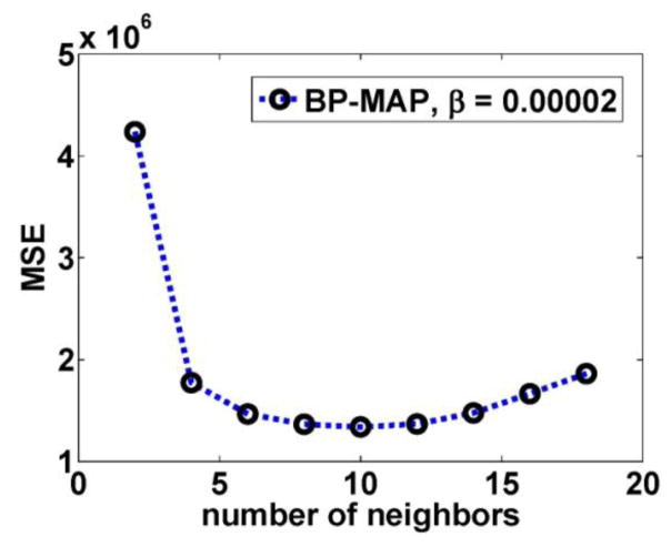
Next, the effect of the number of Bowsher neighbors B and regularization parameter β in the BP-MAP algorithm was studied. The number of neighbors B ranged from 2 to 18 for a 3D neighborhood system with 18 neighbors, and the regularization parameter ranged from 0.000001 to 0.0001. Figure 7 shows the plots of MSE as a function of the regularization parameter for BP-MAP reconstruction. The optimized regularization parameter β can be found by zooming into the marked area; though some curves lead to very similar performance). From figure 7(b), we can see the optimal β value to be around 10−4.7. To provide an more clear demonstration of the effect of number of neighbor B, figure 8 shows the MSE value as a function of the number of neighbors B for BP-MAP reconstructed at 10 iteration (16 subsets) with β=0.00002. We can see that BP-MAP depicts enhanced performance when the number of neighbors B ranges from 8 to 12. Thus, we chose B=10 as the optimal number of neighbors. From figure 6 and figure 7, we can also note that BP-MAP has the least MSE compared with SP-MAP and JP-MAP reconstruction.
Figure 7.
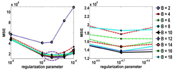
Plots of (a) MSE as a function of the regularization parameter for BP-MAP reconstructed image at 10 iterations (16 subsets) with different number of neighbors B (ranging from 2 to 18), and (b) an enlarged version of the marked region in figure (a).
Figure 8.
Plots of MSE as a function of the number of neighbor B for BP-MAP reconstructed at 10 iteration (16 subsets) with β =0.00002 (corresponding to the regularization equals 10−4.7 in figure 7(b)).
4.1.2. Performance comparison
Following the optimization of parameters, we compared the performance of conventional 3D PET reconstruction (including MLEM, SP-MAP) and proposed MAP reconstruction (JP-MAP). Different scenarios were considered including the use of different noise levels (3%, 9%, and 15%) in the MR images (realistic Rician noise), with and without the additional effect of PET-MR mis-regirstration. To provide an overall performance evaluation of the reconstruction algorithms across the brain, figure 9 depicts plots of overall NSD versus overall Bias for various reconstructed images with different MR image noise levels. It is clearly seen that the MLEM approach results in substantially increased noise levels with increasing iterations, while the SP-MAP approach somewhat reduced the noise levels with similar bias. By comparison, the proposed JP-MAP reconstruction method results in the lowest noise at matched bias for different noise levels in MR images and with the additional effect of PET-MR mis-registration.
Figure 9.
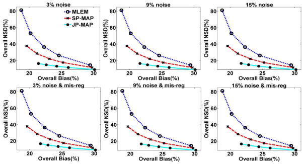
Plots of overall NSD (noise) versus Bias curves of reconstructed brain images (from top to bottom) changing with the iteration number (increasing iterations of 1, 2, 3, 5 and 10 (16 subsets)), using: (i) conventional MLEM reconstruction, (ii) conventional MAP reconstruction (SP-MAP) and (iii) the proposed MAP reconstruction (JP-MAP). Regularization was optimized for both conventional and proposed MAP reconstructions to provide a fair comparison.
In order to provide a more direct visual impression of the reconstructed images (corresponding to figure 9), figure 10 shows transaxial, coronal, and sagittal slices through the images obtained by conventional 3D PET reconstruction (namely MLEM and SP-MAP) and proposed MAP reconstruction (JP-MAP). To enable a fair comparison, we show the MLEM and SP-MAP reconstructed images at 5 iterations and the JP-MAP reconstructed images at 10 iterations (all with 16 subsets), thus the images are approximately matched in bias as in figure 9. It is clearly seen that the MLEM approach results in very noisy images, while SP-MAP reconstruction somewhat reduces the noise levels. By comparison, the reconstructed images using the proposed JP-MAP reconstruction method exhibit clearly improved images for different MR noise levels and mis-registrations.
Figure 10.
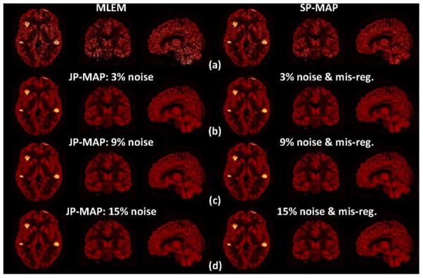
Transaxial/coronal/sagital images: (a) conventional reconstruction (MLEM and SP-MAP), as well as proposed MAP reconstruction (JP-MAP) with (b) 3%, (c) 9% and (d) 15% noise in the MR images, with and without PET/MR mis-registration. Reconstructions included 5 iterations of the MLEM and SP-MAP algorithms, while having 10 iterations of the proposed JP-MAP algorithm (all with 16 subsets), to provide images of nearly matched bias, for fair visual comparison of noise levels.
To evaluate the lesion contrast in the reconstructed images (corresponding to figure 9), figure 11 depicts plots of overall NSD (noise) versus contrast recovery ratio (CRR), as generated using increasing iterations of 1, 2, 3, 5 and 10 (16 subsets), for different reconstruction algorithms. It is seen that the JP-MAP reconstruction images at matched lesion contrast with conventional 3D PET reconstruction (including MLEM, SP-MAP) achieves the lowest noise levels.
Figure 11.
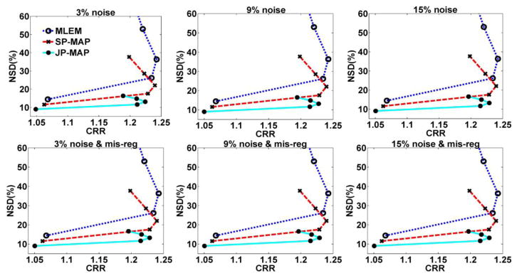
Plots of gray matter NSD (noise) versus lesions overall contrast for reconstructed images (from top to bottom) changing with the iteration number (increasing iterations of 1, 2, 3, 5 and 10 (16 subsets)), using: (i) conventional MLEM reconstruction (MLEM), (ii) conventional MAP reconstruction (SP-MAP), and (iii) proposed MAP reconstruction (JP-MAP).
Next we focused on the comparison of our proposed approach to another MR guided PET image reconstruction method, namely the Bowsher prior. The comparisons are shown in figures 12, 13 and 14. It is worth emphasizing that the Bowsher method was also optimized (number of neighbors, beta, etc.) to perform a fair comparison of the two methods. It is seen in figure 12 that the proposed JP-MAP method depicts quantitative performance that is nearly matched with that of the Bowsher prior reconstruction (BP-MAP) for different noise level in MR images, and in fact slightly better especially in the case of mis-registrations (as explained next). Note that for different noise level (from 3% to 15%) with perfect registration in MR images in figure 12 (top), the BP-MAP performs slightly better than JP-MAP in terms of noise versus bias. However, for all the noise level with mis-registration in figure 12 (bottom), the JP-MAP depicts slightly enhanced robustness and performance compared to BP-MAP in terms of noise versus bias. This can be explained by the fact that the Bowsher prior effectively performs a local “binary” segmentation of MR images, and thus is potentially more vulnerable to inconsistencies between the MR image and the PET image. In any case, the reconstructed images using BP-MAP and proposed JP-MAP reconstruction methods exhibited similar visual performance (not shown).
Figure 12.

Plots of overall NSD (noise) versus Bias for reconstructed images (from top to bottom) changing with the iteration number (increasing iterations of 1, 2, 3, 5 and 10 (16 subsets)), using: (i) MAP reconstruction with the Bowsher prior (BP-MAP) and (iii) the proposed MAP reconstruction with joint-prior (JP-MAP).
Figure 13.
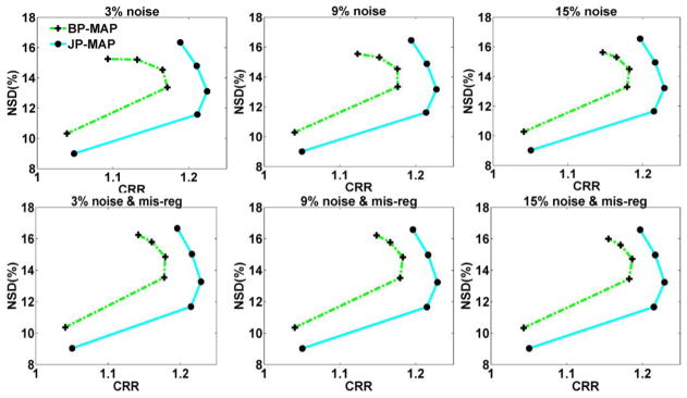
Plots of gray matter overall NSD (noise) versus lesions overall contrast curves of reconstructed brain images (from top to bottom) changing with the iteration number (increasing iterations of 1, 2, 3, 5 and 10 (16 subsets)), using: (i) MAP reconstruction with Bowsher prior (BP-MAP) and (ii) proposed MAP reconstruction with joint-prior (JP-MAP).
Figure 14.

Plots of gray matter NSD (noise) versus lesions contrast recovery ratio (CRR) curves of reconstructed brain images (a–c) changing with the iteration number (increasing iterations of 1, 2, 3, 5 and 10 (16 subsets)) for four lesions, using: (i) MAP reconstruction with Bowsher prior (BP-MAP) and (ii) proposed MAP reconstruction with joint-prior (JP-MAP).
To evaluate the lesion contrast recovery in the reconstructed images, figure 13 shows plots of overall NSD (noise) versus contrast recovery ratio (CRR) in the images as generated using increasing iteration numbers (1, 2, 3, 5 and 10 (16 subsets)), using both BP-MAP and JP-MAP reconstruction algorithms. The JP-MAP reconstruction images depicted slightly reduced noise levels, at matched contrast levels relative to BP-MAP, at different noise levels and more so in the presence of MR-PET mis-registrations.
For further elaboration, figure 14 depicts plots of gray matter NSD (noise) versus lesion contrast recovery ratio for the individual four lesions in the images as generated using increasing iteration numbers (1, 2, 3, 5 and 10 (16 subsets)), using both BP-MAP and JP-MAP reconstruction algorithms with 9% noise in the MR images and PET/MR mis-registration. Similar patterns as in Fig. 13, comparing JP-MAP with BP-MAP, are observed.
To provide an overall performance evaluation of the reconstruction algorithms across the brain, figure 15 depicts plots of overall NSD versus overall Bias for various reconstructed images changing with the increasing regularization parameter β at 10 iterations with mis-registration MR images under noise levels. The BP-MAP reconstruction has better performance than SP-MAP in terms of NSD versus Bias curve. The proposed JP-MAP reconstruction method results in similar performance with BP-MAP reconstruction in terms of NSD versus Bias curve. The BP-MAP reconstruction depicts sensitivity with increasing noise level in MR images, with the curve moving to the right with noise increasing from 3% to 15%. Thus, the JP-MAP reconstruction depicts slightly enhanced robustness with increasing noise levels in MR images.
Figure 15.

Plots of overall NSD (noise) versus Bias curves of reconstructed brain images changing with the increasing regularization parameter β at 10 iterations, using: (i) conventional MAP reconstruction with single hyperbolic prior (SP-MAP), (ii) MAP reconstruction with Bowsher prior (BP-MAP) and (iii) the proposed MAP reconstruction with joint-prior (JP-MAP).
Furthermore, we compared the computational performance of the BP-MAP and JP-MAP reconstruction. For the Bowsher prior computation with N neighborhoods, the computational complexity of the bubble sorting algorithm (in our study) is O(N2), while the computational complexity for the joint prior is O(2N). Though, one may instead perform the sorting algorithm for the Bowsher prior only once, this can pose a huge memory requirement of O(MN), where M is the voxel number of reconstructed image. In our study, on an eight-core Intel Core i7 2600 processor (3.4GHz; 8GB RAM), the JP-MAP reconstruction utilized 72.9 seconds per iteration (each iteration containing 16 subsets), while BP-MAP reconstruction consumed 135.59 seconds per iteration, a significant difference: this analysis obviously incorporated the various steps including forward- and back-projection which are identical for the two algorithms, for a fair, overall comparison of speed performance.
4.2. Application to patient study
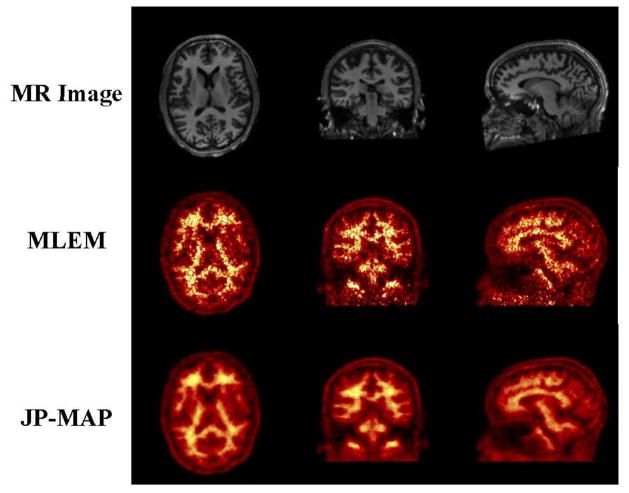
Subsequently, following extensive validations using simulations, we applied the proposed MAP reconstruction method to a Florbetapir patient study on the HRRT scanner (as elaborated in section 3.2). In order to provide a visual comparison of the estimated activity images, figure 16 shows transaxial, coronal and sagittal slices of reconstruction images obtained by conventional MLEM with FWHM=2mm Gaussian filtering and proposed MAP reconstruction algorithms with joint prior (JP). The noise reduction in activity image reconstructed from the proposed approach is clearly observed.
Figure 16.
MR and reconstructed images on 50 year old male subject (Sec. 3.2). From top to bottom: (i) MR image, (ii) standared 3D MLEM reconstruction (MLEM) and (iii) proposed MAP reconstruction with joint prior (JP-MAP). (From left to right): corresponding to transaxial, coronal and sagittal slices, respectively. Post-filtering (FWHM=2mm) was applied to the MLEM images shown. Both MLEM and JP-MAP reconstruction images were at 10 iterations (16 subsets).
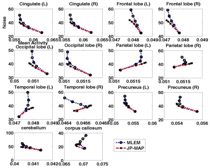
Figure 17 depicts NoiseROI verus ActivityROI plots generated by increasing iterations for 14 individual regions of the brain (cerebellum, corpus callosum, both left (L) and right (R) cingulate, frontal lobe, occipital lobe, parietal lobe and temporal lobe). Across these ROIs, the proposed MAP reconstruction method is commonly seen to quantitatively outperform conventional 3D MLEM reconstruction, in the sense that for a given activity value, improved noise values are attained.
Figure 17.
Plots of regional NSD versus Activity trade-off curves of reconstructed brain images changing with the iteration number (increasing iterations of 1, 2, 3, 5 and 10 (16 subsets)) for different regions, using (i) conventional 3D MLEM reconstruction with FWHM=2mm guassian post-filtering, and (ii) proposed MAP reconstruction with joint prior (JP-MAP)
5. Discussion
5.1. Related work
In a different context of dual-isotope myocardial perfusion SPECT imaging, He et al (2011) proposed a cross-tracer prior that couples voxel values on both images using hyperbolic potential function. Though the authors proposed an iterative algorithm to solve the simultaneous reconstruction problem and arrived at improved results compare with conventional method, the optimization is rather complicated. In any case, the characteristic of the potential function in one image was determined by the voxel intensity difference in another image, which made the potential function sensitive to the voxel intensity differences in the reconstructed image pairs. Wang and Qi (2012) proposed patched-based regularization that used neighborhood patches instead of individual voxel intensity difference to distinguish real edged from noisy fluctuation. In contrast to this, our approach exploits the voxel intensity difference in high-resolution anatomical images to induce the characteristic of the hyperbolic function, which can outperform the single hyperbolic function.
5.2. Selection of the parameter
Selection of a proper regularization parameter β in (4) can be critical for the proposed MAP reconstruction method. Adaptive approaches such as generalized cross validation (GCV), L-curve and maximum likelihood methods impose high computational costs and are not task-based, as we discuss in (Lu et al., 2012). In principle, the parameters δ and η should be threshold values to distinguish edges for PET and MR images, respectively. In our initial study, the δ and η were set to constant values and optimized independently of each other (Lu et al., 2014). However, we found that for each δ, a different optimal value β exists, which makes the optimization strategy more complicated for different η values. In the work (He et al., 2011), for the same value of β and δ (η=δ), the cross-tracer reconstruction does a better job of preserving edges than single hyperbolic prior reconstruction. It allows using a higher value of β, and increasing the smoothing in flat regions with the same edge preservation. This was also oberserved in our initial study (Lu et al., 2014). In this study, we proposed a parameter model, which establish the relationship between the parameter and the mean gradient value of the corresponding image at the n th iteration by a a single parameter α. Thus, it simplify the optimization by reducing the two parameters (δ and η) to one single parameter α. Furthermore, for the same value of β and α, the joint prior reconstruction performs better than single hyperbolic prior reconstruction in terms of MSE, as elaborated in figure 6. In the future, we wish to perform task-based parameter optimization involving observer studies, as well as overall statistical receiver operating characteristic (ROC) analysis to compare the proposed technique with conventional MLEM and MAP image reconstruction method (He et al., 2006).
5.3. Future work
The present work has focus on quantitative analysis and comparison of the different methods in terms of image fidelity. The NSD defined in (18) reflects the mean standard deviation of each voxel across the ROI. However, to quantify mean uptake in each ROI, the NSD may instead be defined to reflect the variability of ROI quantification (i.e. ensemble standard deviation of ROI mean uptake (Rahmim and Tang, 2013)). It is very appropriate in future work to perform specific task performance analysis, including diagnostic detection task performance for the various methods. Future work consists of application to an extensive pool of subject studies on the HRRT scanner, including specific focus on Florbetapir (Amyvid). In fact, training material for clinical readers note that some scans are difficult to interpret due to image noise or image blur. The combination of noise and partial volume effects (PVE), namely the spill over of white matter signal, could create an impression of uptake in gray matter, resulting in a false positive read. We aim to validate the ability to produce enhanced visual reads and enable enhanced quantitative accuracy, including greater concordance with post-mortem studies.
6. Summary
This work proposed an OSL MAP reconstruction method for PET brain imaging to enhance the image reconstruction via introduction of joint priors between anatomical and functional image. We adapted a hyperbolic potential function to incorporating the anatomical information and constructed an anatomy-dependent potential function in the joint prior term. Using realistic simulated 18FDG PET data, we optimize the performance of the proposed JP-MAP PET reconstruction algorithm, and compared its performance with conventional 3D MLEM and SP-MAP reconstruction algorithms. The proposed JP-MAP reconstruction algorithm resulted in quantitatively enhanced reconstructed images, as demonstrated in extensive 18FDG PET simulation study. The proposed method was also tested on a 20 min Florbetapir patient study performed on the high-resolution research tomograph. The proposed method was shown to outperform conventional methods in visual as well as quantitative accuracy improvements (in terms of regional noise versus Activity value performance). The technique was also compared with another MR-guided PET image reconstruction method, namely BP-MAP invoking the Bowsher prior, demonstrating some quantitative enhancement especially in the case of PET-MR mis-registrations, and was seen to result in considerable computational speed-up of overall image reconstruction.
Acknowledgments
This work was supported by the 973 Program of China under grant no. 2010CB732503, NIH grant 1S10RR023623, the Specialized Research Fund for the Doctoral Program of Higher Education under grant 20134433120017, the Medical Scientific Research Foundation of Guangdong Province under grant B2014240, and the National Natural Science Foundation of China under grants 81000613 and 81101046. The authors also wish to thank Drs. Sacktor and Mohamed for providing access to [18F]Florbetapir patient data to evaluate in this work, as collected under support by NIH grant NS081196. The authors also wish to thank Dr. Anil Kumar for help with delineation of ROIs in patient study and Dr. Noble George for helpful discussions.
Contributor Information
Lijun Lu, Email: ljlubme@gmail.com.
Wufan Chen, Email: chenwf@fimmu.com.
Arman Rahmim, Email: arahmim1@jhmi.edu.
References
- Alessio AM, Kinahan PE. Improved quantitation for PET/CT image reconstruction with system modeling and anatomical priors. Med Phys. 2006;33:4095–103. doi: 10.1118/1.2358198. [DOI] [PubMed] [Google Scholar]
- Bai B, Li Q, Leahy RM. Magnetic Resonance Guided Positron Emission Tomography Image Reconstruction. Semin Nucl Med. 2013;43:30–44. doi: 10.1053/j.semnuclmed.2012.08.006. [DOI] [PMC free article] [PubMed] [Google Scholar]
- Bousse A, Pedemonte S, Kazantsev D, Ourselin S, Arridge S, Hutton BF. Weighted MRI-based bowsher priors for SPECT brain image reconstruction. IEEE Nuclear Science Symp Conf Record. 2010:3519–22. [Google Scholar]
- Bowsher JE, Johnson VE, Turkington TG, Jaszczak RJ, Floyd CE, Jr, Coleman RE. Bayesian reconstruction and use of anatomical a priori information for emission tomography. IEEE Trans Med Imaging. 1996;15:673–86. doi: 10.1109/42.538945. [DOI] [PubMed] [Google Scholar]
- Bowsher JE, Yuan H, Hedlund LW, Turkington TG, Akabani G, Badea A, Kurylo WC, Wheeler CT, Cofer GP, Dewhirst MW. Utilizing MRI information to estimate F18-FDG distributions in rat flank tumors. IEEE Nuclear Science Symp Conf Record. 2004:2488–92. [Google Scholar]
- Charbonnier P, Blanc-Feraud L, Aubert G, Barlaud M. Deterministic edge-preserving regularization in computed imaging. IEEE Trans Image Process. 1997;6:298–311. doi: 10.1109/83.551699. [DOI] [PubMed] [Google Scholar]
- Chun SY, Fessler JA, Dewaraja YK. Non-Local Means Methods Using CT side information for I-131 SPECT image reconstruction. IEEE Nuclear Science Symp Conf Record. 2012:3362–6. [Google Scholar]
- Collins DL, Zijdenbos AP, Kollokian V, Sled JG, Kabani NJ, Holmes CJ, Evans AC. Design and construction of a realistic digital brain phantom. IEEE Trans Med Imaging. 1998;17:463–8. doi: 10.1109/42.712135. [DOI] [PubMed] [Google Scholar]
- Comtat C, Kinahan PE, Fessler JA, Beyer T, Townsend DW, Defrise M, Michel C. Clinically feasible reconstruction of 3D whole-body PET/CT data using blurred anatomical labels. Phys Med Biol. 2002;47:1–20. doi: 10.1088/0031-9155/47/1/301. [DOI] [PubMed] [Google Scholar]
- Fessler JA, Clinthorne NH, Rogers WL. Regularized emission image reconstruction using imperfect side information. IEEE Trans Nucl Sci. 1992;39:1464–71. [Google Scholar]
- Geman S, Geman D. Stochastic relaxation, Gibbs distributions, and the Bayesian restoration of images. IEEE Trans Pattern Anal Mach Intell. 1984;13:413–25. doi: 10.1109/tpami.1984.4767596. [DOI] [PubMed] [Google Scholar]
- Gravel P, Verhaeghe J, Reader AJ. 3D PET image reconstruction including both motion correction and registration directly into an MR or stereotaxic spatial atlas. Phys Med Biol. 2013;58:105–26. doi: 10.1088/0031-9155/58/1/105. [DOI] [PubMed] [Google Scholar]
- Green PJ. Bayesian reconstructions from emission tomography data using a modified EM algorithm. IEEE Trans Med Imaging. 1990;9:84–93. doi: 10.1109/42.52985. [DOI] [PubMed] [Google Scholar]
- He X, Cheng L, Fessler JA, Frey EC. Regularized image reconstruction algorithms for dual-isotope Myocardial Perfusion SPECT (MPS) imaging Using a Cross-Tracer Prior. IEEE Trans Med Imaging. 2011;30:1169–83. doi: 10.1109/TMI.2010.2087031. [DOI] [PMC free article] [PubMed] [Google Scholar]
- He X, Metz CE, Tsui BM, Links JM, Frey EC. Three-class ROC analysis-A decision theoretic approach under the ideal observer framework Medical Imaging. IEEE Trans Med Imaging. 2006;25:571–81. doi: 10.1109/tmi.2006.871416. [DOI] [PubMed] [Google Scholar]
- Kazantsev D, Bousse A, Pedemonte S, Arridge SR, Hutton BF, Ourselin S. Edge preserving Bowsher prior with nonlocal weighting for 3D SPECT reconstruction. IEEE Int Symp Biomed Imaging. 2011:1158–61. [Google Scholar]
- Leahy RM, Qi J. Statistical approaches in quantitative positron emission tomography. Stat Comput. 2000;10:147–65. [Google Scholar]
- Lipinski B, Herzog H, Rota Kops E, Oberschelp W, Muller-Gartner HW. Expectation maximization reconstruction of positron emission tomography images using anatomical magnetic resonance information. IEEE Trans Med Imaging. 1997;16:129–36. doi: 10.1109/42.563658. [DOI] [PubMed] [Google Scholar]
- Lu L, Karakatsanis NA, Tang J, Chen W, Rahmim A. 3.5D dynamic PET image reconstruction incorporating kinetics-based clusters. Phys Med Biol. 2012;57:5035–55. doi: 10.1088/0031-9155/57/15/5035. [DOI] [PMC free article] [PubMed] [Google Scholar]
- Lu L, Ma J, Feng Q, Chen W, Rahmim A. Quantitative brain PET imaging incorporating an anatomy-guided joint prior model. J Nucl Med. 2014;55:370. doi: 10.1088/0031-9155/60/6/2145. [DOI] [PMC free article] [PubMed] [Google Scholar]
- Lu L, Ma J, Huang J, Zhang H, Bian Z, Chen W, Liang Z. Generalized metrics induced anatomical prior for MAP PET image reconstruction. Proc Int Meeting on Fully 3D Image Recon in Rad and Nucl Med. 2011:233–6. [Google Scholar]
- Lu L, Ma J, Tang J, Feng Q, Rahmim A, Chen W. Anatomy-guided brain PET imaging incorporating a joint prior model. IEEE 11th International Symposium on Biomedical Imaging (ISBI) 2014:959–62. [Google Scholar]
- Mohy-ud-Din H, Karakatsanis NA, Ay MR, Endres CJ, Wong DF, Rahmim A. Generalized inter-frame and intra-frame motion correction in pet imaging-a simulation study. IEEE Nuclear Science Symp Conf Record. 2011:3858–62. [Google Scholar]
- Mumcuoğlu EU, Leahy R, MandCherry SR. Bayesian reconstruction of PET images: methodology and performance analysis. Phys Med Biol. 1996;41:1777–807. doi: 10.1088/0031-9155/41/9/015. [DOI] [PubMed] [Google Scholar]
- Nguyen VG, Lee SJ. Incorporating anatomical side information into PET reconstruction using nonlocal regularization. IEEE Trans Image Process. 2013;22:3961–73. doi: 10.1109/TIP.2013.2265881. [DOI] [PubMed] [Google Scholar]
- Nuyts J. The use of mutual information and joint entropy for anatomical priors in emission tomography. IEEE Nuclear Science Symp Conf Record. 2007:4149–54. [Google Scholar]
- Rahmim A, Tang J. Noise propagation in resolution modeled PET imaging and its impact on delectability. Phys Med Biol. 2013;58:6945–968. doi: 10.1088/0031-9155/58/19/6945. [DOI] [PMC free article] [PubMed] [Google Scholar]
- Rahmim A, Zaidi H. PET versus SPECT: strengths, limitations and challenges. Nucl Med Commun. 2008;29:193–207. doi: 10.1097/MNM.0b013e3282f3a515. [DOI] [PubMed] [Google Scholar]
- Rahmim A, Cheng JC, Blinder S, Camborde ML, Sossi V. Statistical dynamic image reconstruction in state-of-the-art high-resolution PET. Phys Med Biol. 2005;50:4887–912. doi: 10.1088/0031-9155/50/20/010. [DOI] [PubMed] [Google Scholar]
- Rangarajan A, Hsiao T, Gindi G. A Bayesian joint mixture framework for the integration of anatomical information in functional image reconstruction. J Math Imaging Vis. 2000;12:199–217. [Google Scholar]
- Sastry S, Carson RE. Multimodality Bayesian algorithm for image reconstruction in positron emission tomography: a tissue composition model. IEEE Trans Med Imaging. 1997;16:750–61. doi: 10.1109/42.650872. [DOI] [PubMed] [Google Scholar]
- Slomka PJ, Baum RP. Multimodality image registration with software: state-of-the-art. Eur J Nucl Med Mol I. 2009;36:44–55. doi: 10.1007/s00259-008-0941-8. [DOI] [PubMed] [Google Scholar]
- Somayajula S, Panagiotou C, Rangarajan A, Li Q, Arridge SR, Leahy RM. PET image reconstruction using information theoretic anatomical priors. IEEE Trans Med Imaging. 2011;30:537–49. doi: 10.1109/TMI.2010.2076827. [DOI] [PMC free article] [PubMed] [Google Scholar]
- Sossi V, de Jong HW, Barker WC, Bloomfield P, Burbar Z, Camborde M, Comtat C, Eriksson LA, Houle S, Keator D. The second generation HRRT-a multi-centre scanner performance investigation. IEEE Nuclear Science Symp Conf Record. 2005:2195–9. [Google Scholar]
- Tang J, Rahmim A. Anatomy assisted MAP-EM PET image reconstruction incorporating joint entropies of wavelet subband image pairs. IEEE Nuclear Science Symp Conf Record. 2009a:3741–5. [Google Scholar]
- Tang J, Rahmim A. Bayesian PET image reconstruction incorporating anato-functional joint entropy. Phys Med Biol. 2009b;54:7063–75. doi: 10.1088/0031-9155/54/23/002. [DOI] [PMC free article] [PubMed] [Google Scholar]
- Van de Sompel D, Brady M. Regularising limited view tomography using anatomical reference images and information theoretic similarity metrics. Med Image Anal. 2012;16:278–300. doi: 10.1016/j.media.2011.08.005. [DOI] [PubMed] [Google Scholar]
- Vunckx K, Atre A, Baete K, Reilhac A, Deroose CM, Van Laere K, Nuyts J. Evaluation of three MRI-based anatomical priors for quantitative PET brain imaging. IEEE Trans Med Imaging. 2012;31:599–612. doi: 10.1109/TMI.2011.2173766. [DOI] [PubMed] [Google Scholar]
- Wang G, Qi J. Penalized likelihood PET image reconstruction using patch-based edge-preserving regularization. IEEE Trans Med Imaging. 2012;31:2194–204. doi: 10.1109/TMI.2012.2211378. [DOI] [PMC free article] [PubMed] [Google Scholar]
- Yang L, Rieves D, Ganley C. Brain amyloid imaging—FDA approval of florbetapir F18 injection. New Engl J Med. 2012;367:885–7. doi: 10.1056/NEJMp1208061. [DOI] [PubMed] [Google Scholar]


