Generalized species sampling priors with latent Beta reinforcements

Abstract

Many popular Bayesian nonparametric priors can be characterized in terms of exchangeable species sampling sequences. However, in some applications, exchangeability may not be appropriate. We introduce a novel and probabilistically coherent family of non-exchangeable species sampling sequences characterized by a tractable predictive probability function with weights driven by a sequence of independent Beta random variables. We compare their theoretical clustering properties with those of the Dirichlet Process and the two parameters Poisson-Dirichlet process. The proposed construction provides a complete characterization of the joint process, differently from existing work. We then propose the use of such process as prior distribution in a hierarchical Bayes modeling framework, and we describe a Markov Chain Monte Carlo sampler for posterior inference. We evaluate the performance of the prior and the robustness of the resulting inference in a simulation study, providing a comparison with popular Dirichlet Processes mixtures and Hidden Markov Models. Finally, we develop an application to the detection of chromosomal aberrations in breast cancer by leveraging array CGH data.

1. INTRODUCTION

All authors have equally contributed to the manuscript.

Bayesian nonparametric priors have become increasingly popular in applied statistical modeling in the last few years. Examples of their wide area of applications range from variable selection in genetics (Kim et al., 2006) to linguistics (Teh, 2006b; Wallach et al., 2008), psychology (Navarro et al., 2006), human learning (Griffiths, 2007), image segmentation (Sudderth and Jordan, 2009) and applications to the neurosciences (Jbabdi et al., 2009). See also Hjort et al. (2010). The increased interest in non-parametric Bayesian approaches is motivated by a number of attractive inferential properties. For example, Bayesian nonparametric priors are often used as flexible models to describe the heterogeneity of the population of interest, as they implicitly induce a clustering of the observations into homogeneous groups. Such a clustering can be seen as a realization of a random partition scheme and can often be characterized in terms of a species sampling (SS) allocation rule. More formally, a SS sequence is a sequence of random variables X₁, X₂, … , characterized by the predictive probability functions,

$$\mathit{P}\mathrm{\{}{\mathit{X}}_{\mathit{n}\mathrm{+}\mathrm{1}}\mathrm{\in }\mathrm{\cdot }\mathrm{|}{\mathit{X}}_{\mathrm{1}}\mathrm{,}\mathrm{}\mathrm{\text{...}}\mathrm{,}\mathrm{}{\mathit{X}}_{\mathit{n}}\mathrm{\}}\mathrm{=}{\displaystyle \sum }_{\mathit{j}\mathrm{=}\mathrm{1}}^{\mathit{n}}{\mathit{q}}_{\mathit{n}\mathrm{,}\mathit{j}}{\mathit{\delta }}_{{\mathit{X}}_{\mathit{j}}}\mathrm{(}\mathrm{\cdot }\mathrm{)}\mathrm{+}{\mathit{q}}_{\mathit{n}\mathrm{,}\mathit{n}\mathrm{+}\mathrm{1}}{\mathit{G}}_{\mathrm{0}}\mathrm{(}\mathrm{\cdot }\mathrm{),}$$ (1)

where δ_x(·) denotes a point mass at x, q_n,j (j = 1, … , n + 1) are non–negative functions of (X₁, … , X_n), or weights, such that ${{\displaystyle \sum }}_{\mathit{j}\mathrm{=}\mathrm{1}}^{\mathit{n}\mathrm{+}\mathrm{1}}{\mathit{q}}_{\mathit{n}\mathrm{,}\mathit{j}}\mathrm{=}\mathrm{1,}$, and G₀ is a non-atomic probability measure (Pitman, 1996b). Collecting the unique values of X_j, (1) can be rewritten as

$$\mathit{P}\mathrm{\{}{\mathit{X}}_{\mathit{n}\mathrm{+}\mathrm{1}}\mathrm{\in }\mathrm{\cdot }\mathrm{|}{\mathit{X}}_{\mathrm{1}}\mathrm{,}\mathrm{}\mathrm{\text{...}}\mathrm{,}\mathrm{}{\mathit{X}}_{\mathit{n}}\mathrm{\}}\mathrm{=}{\displaystyle \sum }_{\mathit{j}\mathrm{=}\mathrm{1}}^{{\mathit{K}}_{\mathit{n}}}{\mathit{q}}_{\mathit{j}}^{\mathrm{*}}{\mathit{\delta }}_{{\mathit{X}}_{\mathit{j}}^{\mathrm{*}}}\mathrm{(}\mathrm{\cdot }\mathrm{)}\mathrm{+}{\mathit{q}}_{{\mathit{K}}_{\mathit{n}}\mathrm{+}\mathrm{1}}^{\mathrm{*}}{\mathit{G}}_{\mathrm{0}}\mathrm{(}\mathrm{\cdot }\mathrm{),}$$ (2)

where K_n is the (random) number of distinct values, say $\mathrm{(}{\mathit{X}}_{\mathrm{1}}^{\mathrm{*}}\mathrm{,}\mathrm{}\mathrm{\text{...}}{\mathit{X}}_{{\mathit{K}}_{\mathit{n}}}^{\mathrm{*}}\mathrm{)}$, in the vector X(n) = (X₁, … , X_n) and ${\mathit{q}}_{\mathit{j}}^{\mathrm{*}}$ are suitable non–negative weights. In particular, an exchangeable SS sequence is characterized by weights ${\mathit{q}}_{\mathit{j}}^{\mathrm{*}}$ that depend only on n_n = (n_1n, … , n_Knn), where n_jn is the frequency of ${\mathit{X}}_{\mathit{j}}^{\mathrm{*}}$ in X(n) (Fortini et. al, 2000; Hansen and Pitman, 2000; Lee et al., 2008). The most well known example of predictive rules of type (1) is the Blackwell MacQueen sampling rule, which implicitly defines a Dirichlet Process (DP, Blackwell and MacQueen, 1973; Ishwaran and Zarepour, 2003). The predictive rule characterizing a DP with mass parameter θ and base measure G₀(·), DP(θ, G₀), sets ${\mathit{q}}_{\mathit{n}\mathrm{,}\mathit{j}}\mathrm{=}\frac{\mathrm{1}}{\mathit{n}\mathrm{+}\mathit{\theta }}$ and ${\mathit{q}}_{\mathit{n}\mathrm{,}\mathit{n}\mathrm{+}\mathrm{1}}\mathrm{=}\frac{\mathit{\theta }}{\mathit{n}\mathrm{+}\mathit{\theta }}$ in (1).

Whenever the weights ${\mathit{q}}_{\mathit{j}}^{\mathrm{*}}\mathrm{(}{\mathrm{n}}_{\mathit{n}}\mathrm{)}$ and ${\mathit{q}}_{{\mathit{K}}_{\mathit{n}}\mathrm{+}\mathrm{1}}^{\mathrm{*}}\mathrm{(}{\mathrm{n}}_{\mathit{n}}\mathrm{)}$ do not depend only on n_n, the sequence (X₁, X₂, …) is not exchangeable. Models with non-exchangeable random partitions have recently appeared in the literature, e.g. to allow for partitions that depend on covariates. Park and Dunson (2007) derive a generalized product partition model (GPPM) in which the partition process is predictor–dependent. Their GPPM generalizes the DP clustering mechanism to relax the exchangeability assumption through the incorporation of predictors, implicitly defining a generalized Pólya urn scheme. Müller and Quintana (2010) define a product partition model that includes a regression on covariates, allowing units with similar covariates to have greater probability of being clustered together. Arguably, the previous models provide an implicit modification of the predictive rule (1) where the weights can be seen as function of some external predictor. Alternatively, other authors model the weights q_j (n_n) explicitly, for instance, by specifying the weights as a function of the distance between data points (Dahl et al., 2008; Blei and Frazier, 2011). However, the general properties of the random partitions generated by such processes have not been specifically addressed.

In this paper, we introduce a novel and probabilistically coherent family of non-exchangeable species sampling sequences, where the weights are specified sequentially and do not depend on the cluster sizes, but instead they depend on the realizations of a set of latent variables. Working within this family, we propose a simple characterization of the weights in the predictive probability function as a product of independent Beta random variables. This strategy leads to a well-defined random allocation scheme for the observables. The resulting process, which we call Beta-GOS process, is a special case of a Generalized Ottawa Sequence (GOS), recently introduced by Bassetti et al. (2010).

In Section 2, we discuss the properties of the Beta-GOS process, with particular regard to the clustering induced on the observables. In Section 3, we study the asymptotic distribution of the (random) number of distinct values in the sequence, K_n, for some natural specifications of the weights, and we compare those results with the well-known asymptotic results characterizing the DP and the two-parameters Poisson Dirichlet process. In many applications, nonparametric processes are often used within hierarchical models to specify the prior distribution of some parameters of the distribution of the observables. For example, this is a popular use for mixtures of Dirichlet Processes. Similarly, the Beta-GOS process can also be used to define a prior in a hierarchical model. In Section 4, we outline a basic hierarchical model based on the Beta-GOS process and we outline the basic steps of a MCMC sampler for posterior inference. In Section 5, we design a set of simulations to we compare the behavior of the Beta-GOS model with that of DP mixtures and hidden Markov Models (HMM) in terms of cluster estimation. Our results suggest that the Beta-GOS can be seen as a robust alternative to the Dirichlet process when exchangeability would be hardly justified in practice, but still there is a need to describe the heterogeneity of our observations by virtue of an unsupervised clustering of the data. The Beta-GOS also provides an alternative to customary HMM, especially when the number of states is unknown or the Markovian structure is expected to vary with time.

In Section 6, we analyze two published data sets of genomic and transcriptional aberrations (Chin et al., 2006; Curtis et al., 2012). Bayesian models for Array CGH data have been recently investigated by Guha et al. (2008), DeSantis et al. (2009), Baladandayuthapani et al. (2010), Du et al (2010), Cardin et al. (2011), and Yau et al. (2011), among others. Guha et al. propose a four state homogenous Bayesian HMM to detect copy number amplifications and deletions and partition tumor DNA into regions (clones) of relatively stable copy number. DeSantis et al. extend this approach and develop a supervised Bayesian latent class approach for classification of the clones that relies on a heterogenous hidden Markov model to account for local dependence in the intensity ratios. In a heterogeneous hidden Markov model, the transition probabilities between states depend on each single clone or the the distance between adjacent clones (Marioni et al., 2006). Du et al. propose a sticky Hierarchical DP-HMM (Fox et al., 2011; Teh et al., 2006a) to infer the number of states in an HMM, while also imposing state persistence. Yau et al. (2011) also propose a nonparametric Bayesian HMM, but use instead a DP mixture to model the likelihood in each state. With respect to those proposals, we also assume that the number of states is unknown, as it is typical in a Bayesian nonparametric setting, but we don’t need a parameter to explicitly account for state persistence. This is because the Beta-GOS model is “non-homogenous” by design, as the weights in the species sampling mechanisms adapt to take into account the local dependence in the clones’ intensities. We show that the Beta-GOS is able to identify clones that have been linked to breast cancer pathophysiologies in the medical literature.

We conclude with some final remarks in Section 7. Technical details and proofs of theorems and lemmas are provided in the Appendix.

2. THE BETA-GOS PROCESS

As anticipated, the Beta-GOS process is defined by a modification of the predictive rule that characterizes the species sampling mechanism (1), where the weights are a product of independent Beta random variables. More in general, we start considering a sequence of random variables (X_n)_n≥1 characterized by the predictive distributions

$$\mathit{P}\mathrm{\{}{\mathit{X}}_{\mathit{n}\mathrm{+}\mathrm{1}}\mathrm{\in }\mathrm{\cdot }\mathrm{|}\mathit{X}\mathrm{(}\mathit{n}\mathrm{)}\mathrm{,}\mathrm{}\mathit{W}\mathrm{(}\mathit{n}\mathrm{)}\mathrm{\}}\mathrm{=}{\displaystyle \sum }_{\mathit{j}\mathrm{=}\mathrm{1}}^{\mathit{n}}{\mathit{p}}_{\mathit{n}\mathrm{,}\mathit{j}}{\mathit{\delta }}_{{\mathit{X}}_{\mathit{j}}}\mathrm{(}\mathrm{\cdot }\mathrm{)}\mathrm{+}{\mathit{r}}_{\mathit{n}}{\mathit{G}}_{\mathrm{0}}\mathrm{(}\mathrm{\cdot }\mathrm{)}$$ 3

where W(n) = (W₁, … , W_n) is a vector of independent random variables W_k taking values in [0, 1], and the weights are defined by

$${\mathit{p}}_{\mathit{n}\mathrm{,}\mathit{j}}\mathrm{:}\mathrm{=}\mathrm{(}\mathrm{1}\mathrm{-}{\mathit{W}}_{\mathit{j}}\mathrm{)}\underset{\mathit{i}\mathrm{=}\mathit{j}\mathrm{+}\mathrm{1}}{\overset{\mathit{n}}{{\displaystyle \Pi }}}{\mathit{W}}_{\mathit{i,}}{\mathit{r}}_{\mathit{n}}\mathrm{:}\mathrm{=}\underset{\mathit{i}\mathrm{=}\mathrm{1}}{\overset{\mathit{n}}{{\displaystyle \Pi }}}{\mathit{W}}_{\mathit{i.}}$$ 4

The prediction rule (3) defines a special case of a Generalized Ottawa Sequence, introduced in Bassetti et al. (2010), a type of Generalized Pólya Urn sequences where the reinforcement is randomly determined by the realizations of a latent process (see also Guha, 2010, for an alternative proposal). Except from a few special cases, the X_i’s in a GOS are not exchangeable. However, it can be shown that these sequences maintain some properties typical of exchangeable sequences. Most notably, any GOS is conditionally identically distributed (CID), i.e. for all n > 0, the X_n+j ’s, j ≥ 1, are identically distributed, conditionally on (X₁, … , X_n, W₁, … , W_n). Hence, the X_i’s are also marginally identically distributed. Note that a CID sequence is not necessarily stationary. If a CID sequence is also stationary then it is exchangeable. Finally, although no representation theorem is known for CID sequences, it can be shown that given any bounded and measurable function f , the predictive mean E[f(X_n+1)|X₁, …, X_n] and the empirical mean $\frac{\mathrm{1}}{\mathit{n}}{{\displaystyle \sum }}_{\mathit{i}\mathrm{=}\mathrm{1}}^{\mathit{n}}{\mathit{X}}_{\mathit{i}}$ converge to the same limit as n goes to infinity. For details, see Berti et al. (2004), where CID sequences have been first introduced. The predictive rule (3) reduces to known cases with a suitable choice of the latent W_n’s; for instance if W_n := (θ + n − 1)/(θ + n), then (3) coincides with the Blackwell-MacQueen sampling rule characterizing a DP (θ, G₀).

In this paper, we propose (W_n)_n≥1 be a sequence of independent Beta(α_n, β_n) random variables and we call the resulting (X₁, X₂, …) a Beta-GOS sequence. The choice of Beta latent variables allows for a flexible specification of the species sampling weights, while retaining a simple and interpretable model together with computational simplicity (see later Sections). The allocation rule can also be described in terms of a preferential attachment scheme, where each observation is attached to any of the preceding by means of a “geometric-type” assignment. In this scheme, every individual X_i is characterized by a random weight (or “mark”), 1 − W_i. We can interpret each individual mark as an individual specific attractivity index, as it determines the probability that the next observation will be clustered with X_i. More precisely, the first individual is assigned a random value (or “tag”) X₁, according to G₀. Now, suppose we have X₁, … , X_n together with their marks up to time n, (1 − W₁, … , 1 − W_n). Then, the (n + 1)-th individual will be assigned the same tag as X_n with probability 1 − W_n; the probability of pairing X_n+1 to X_n−1 will be W_n(1 − W_n−1), and so forth. In general, p_n,j will be the product of the repulsions W_i for the latest n − j subjects and the jth attractivity 1 − W_j . Summarizing, X_n+1 will result in a new tag (i.e., X_n+1 ~ G₀) with probability r_n, or will be clustered together with a previously observed tag, say ${\mathit{X}}_{\mathit{k}}^{\mathrm{*}}$, with probability ${{\displaystyle \sum }}_{\mathit{j}\mathrm{:}{\mathit{X}}_{\mathit{j}}\mathrm{=}{\mathit{X}}_{\mathit{k}}^{\mathrm{*}}}{\mathit{p}}_{\mathit{n}\mathrm{,}\mathit{j}}$. In the next Section, we discuss the clustering behavior induced by different specifications of the Beta weights in more detail.

3. CLUSTERING BEHAVIOR OF THE BETA-GOS

The predictive rule (3) implicitly defines a random partition of the set {1, … , n} into K_n blocks. In probability theory, K_n is also referred to as the length of the partition. Knowledge of the behavior of K_n is useful to understand the clustering structure implied by (3). For instance, for a DP (θ, G₀), it is well-known that K_n/ log(n) converges almost surely to a constant, indeed the mass parameter θ. This asymptotic behavior is sometimes described as a “self-averaging” property of the partition (Aoki, M., 2008). From a practical point of view, since K_n/ log(n) converges to a constant, then in the limit K_n is essentially θ log(n); thus, for modeling purposes it suffices to consider only the first moment of K_n. In the case of the two parameter Poisson Dirichlet process the length of the partition K_n (suitably rescaled) converges instead to a random variable. More precisely, for a PD(α, θ), with 0 < α < 1, θ > −α, then K_n/n^α converges a.s. to a strictly positive random variable (see Theorem 3.8 in Pitman, 2006). Therefore, the PD sequence is non self-averaging. When the limit of K_n is essentially a random variable, extra care is needed in the prior assessment of the parameters of the non-parametric prior, since the clustering behavior is ultimately governed by the whole distribution of the limit random variable. For the Beta-GOS process, we focus on the following two cases:

1. α_n = a > 0 and β_n = b > 0 for all n ≥ 1;

2. α_n = θ − 1 + n (θ > 0) and β_n ≥ 1 for all n ≥ 1 .

Then, we can prove the following

Proposition 1. Let K_n be the length of the partition induced by a Beta-GOS, with G₀ non-atomic and W_n ~ Beta(α_n, β_n) (n ≥ 1).

1. If α_n = n + θ − 1, β_n = 1, for given θ > 0, K_n/ log(n) converges in distribution to a Gamma(θ, 1) random variable.

2. If α_n = n + θ − 1, β_n = β, (θ > 0, β > 1) or if α_n = a, β_n = b, (a > 0, b > 0), then K_n converges almost surely to a finite random variable K_∞. In particular, if α_n = a, β_n = b, then

   $$\mathit{E}\mathrm{\left[}{\mathit{e}}^{\mathrm{-}\mathit{t}{\mathit{K}}_{\mathrm{\infty }}}\mathrm{\right]}\mathrm{=}{\mathit{e}}^{\mathrm{-}\mathit{t}}{\displaystyle \sum }_{\mathit{m}\mathrm{\ge }\mathrm{0}}^{\mathit{}}\mathrm{(}\mathit{e}\mathrm{-}\mathit{t}\mathrm{-}\mathrm{1}\mathrm{)}\mathit{m}\underset{\mathit{j}\mathrm{=}\mathrm{1}}{\overset{\mathit{m}}{{\displaystyle \Pi }}}\frac{\mathrm{(}\mathit{a}\mathrm{)}\mathrm{(}\mathit{j}\mathrm{)}}{\mathrm{(}\mathit{a}\mathrm{+}\mathit{b}\mathrm{)}\mathrm{(}\mathit{j}\mathrm{)}\mathrm{-}\mathrm{(}\mathit{a}\mathrm{)}\mathrm{(}\mathit{j}\mathrm{)}}$$

   where (t)^(m) = t(t + 1) … (t + m − 1) and

   $$\mathit{E}\mathrm{[}\mathrm{(}{\mathit{K}}_{\mathrm{\infty }}\mathrm{-}\mathrm{1}\mathrm{)}\mathrm{\text{...}}\mathrm{(}{\mathit{K}}_{\mathrm{\infty }}\mathrm{-}\mathit{m}\mathrm{)}\mathrm{]}\mathrm{=}\mathit{m}\mathrm{!}\underset{\mathit{j}\mathrm{=}\mathrm{1}}{\overset{\mathit{m}}{{\displaystyle \Pi }}}\frac{\mathrm{(}\mathit{a}\mathrm{)}\mathrm{(}\mathit{j}\mathrm{)}}{\mathrm{(}\mathit{a}\mathrm{+}\mathit{b}\mathrm{)}\mathrm{(}\mathit{j}\mathrm{)}\mathrm{-}\mathrm{(}\mathit{a}\mathrm{)}\mathrm{(}\mathit{j}\mathrm{).}}$$

The proof is detailed in the Appendix, where we also provide a general formula for the probability distribution, the k-th moment and the generating function of K_n. The result in Proposition 1(a) represents a case of a quite natural (non exchangeable) partition model for which the length K_n scale as log(n) but is not self-averaging. When α_n = a, β_n = b, according to Proposition 1(b), the convergence of K_n to a finite random variable naturally implies the creation of a few big clusters, as n increases. Instead, for α_n = n + θ − 1, β_n = 1, the mean length of the partition depends on the value of θ, since a bigger number of clusters is associated on average with greater values of θ. However, as θ increases so does the asymptotic variability of K_n; therefore, in this case, a Beta-GOS process can be used to represent uncertainty on K_n (by the lack of the self-averaging property of the process. By means of simulations, we have also confirmed that, for small values of θ, the partition of n elements is skewed, i.e. it is characterized by a small number of big clusters as well as a few small clusters. As θ increases, the sizes of the clusters decrease accordingly, the observations being grouped into clusters of relatively fewer elements. This is similar to what happens for the DP, and indeed in this case the parameter θ could be interpreted as a mass parameter for the Beta-GOS.

The parameters of the W_i’s can be chosen to model the autocorrelation expected a priori in the dynamics of the sequence. The probability of a tie may decrease with n and atoms that have been observed at farthest times may have a greater probability to be selected if they have also been observed more recently. Such considerations may be helpful to guide prior assessment of the Beta hyper-parameters. For given n ≥ 1, taking expectations with respect to the weights W_i’s we obtain

$$\mathit{E}\mathrm{\left[}{\mathit{r}}_{\mathit{n}}\mathrm{\right]}\mathrm{=}\underset{\mathit{j}\mathrm{=}\mathrm{1}}{\overset{\mathit{n}}{{\displaystyle \Pi }}}\frac{{\mathit{\alpha }}_{\mathit{j}}}{{\mathit{\alpha }}_{\mathit{j}}\mathrm{+}{\mathit{\beta }}_{\mathit{j}}}\mathit{E}\mathrm{\left[}{\mathit{p}}_{\mathit{n}\mathrm{,}\mathit{k}}\mathrm{\right]}\mathrm{=}\frac{{\mathit{\beta }}_{\mathit{k}}}{{\mathit{\alpha }}_{\mathit{k}}\mathrm{+}{\mathit{\beta }}_{\mathit{k}}}\underset{\mathit{j}\mathrm{=}\mathit{k}\mathrm{+}\mathrm{1}}{\overset{\mathit{n}}{{\displaystyle \Pi }}}\frac{{\mathit{\alpha }}_{\mathit{j}}}{{\mathit{\alpha }}_{\mathit{j}}\mathrm{+}{\mathit{\beta }}_{\mathit{j}}}\mathit{k}\mathrm{=}\mathrm{1}\mathrm{\text{...}}\mathit{n}$$ (5)

Under (a), it follows that E[r_n] = (a/(a + b))ⁿ and E[p_n,k] = (a/(a + b))^n−k (b/(a + b)); hence, the probabilities of ties depend only on the lag n − k and decrease exponentially as a function of n − k. Under (b),

$$\mathit{E}\mathrm{\left[}{\mathit{r}}_{\mathit{n}}\mathrm{\right]}\mathrm{=}\underset{\mathit{j}\mathrm{=}\mathrm{1}}{\overset{\mathit{n}}{{\displaystyle \Pi }}}\frac{\mathit{j}\mathrm{+}\mathit{\theta }\mathrm{-}\mathrm{1}}{\mathit{j}\mathrm{+}\mathit{\theta }\mathrm{-}\mathrm{1}\mathrm{+}\mathit{\beta }}\mathrm{=}\frac{\mathrm{\Gamma }\mathrm{(}\mathit{\theta }\mathrm{+}\mathit{n}\mathrm{)}\mathrm{\Gamma }\mathrm{(}\mathit{\theta }\mathrm{+}\mathit{\beta }\mathrm{)}}{\mathrm{\Gamma }\mathrm{(}\mathit{\theta }\mathrm{+}\mathit{\beta }\mathrm{+}\mathit{n}\mathrm{)}\mathrm{\Gamma }\mathrm{(}\mathit{\theta }\mathrm{)}}$$

$$\mathit{E}\mathrm{\left[}{\mathit{p}}_{\mathit{n}\mathrm{,}\mathit{k}}\mathrm{\right]}\mathrm{=}\frac{\mathit{\beta }}{\mathit{k}\mathrm{+}\mathit{\theta }\mathrm{-}\mathrm{1}\mathrm{+}\mathit{\beta }}\underset{\mathit{j}\mathrm{=}\mathit{k}\mathrm{+}\mathrm{1}}{\overset{\mathit{n}}{{\displaystyle \Pi }}}\frac{\mathit{j}\mathrm{+}\mathit{\theta }\mathrm{-}\mathrm{1}}{\mathit{j}\mathrm{+}\mathit{\theta }\mathrm{-}\mathrm{1}\mathrm{+}\mathit{\beta }}\mathrm{=}\mathit{\beta }\frac{\mathrm{\Gamma }\mathrm{(}\mathit{\theta }\mathrm{+}\mathit{n}\mathrm{)}\mathrm{\Gamma }\mathrm{(}\mathit{\theta }\mathrm{-}\mathrm{1}\mathrm{+}\mathit{\beta }\mathrm{+}\mathit{k}\mathrm{)}}{\mathrm{\Gamma }\mathrm{(}\mathit{\theta }\mathrm{+}\mathit{\beta }\mathrm{+}\mathit{n}\mathrm{)}\mathrm{\Gamma }\mathrm{(}\mathit{\theta }\mathrm{+}\mathit{k}\mathrm{)}}\mathit{k}=1,...\mathit{n.}$$

Thus, for n, k → + ∞, $\mathit{E}\mathrm{\left[}{\mathit{r}}_{\mathit{n}}\mathrm{\right]}\mathrm{~}\frac{\mathrm{1}}{{\mathit{n}}^{\mathit{\beta }}}$ and $\mathit{E}\mathrm{\left[}{\mathit{p}}_{\mathit{n}\mathrm{,}\mathit{k}}\mathrm{\right]}\mathrm{~}\frac{{\mathit{k}}^{\mathit{\beta }\mathrm{-}\mathrm{1}}}{{\mathit{n}}^{\mathit{\beta }}}$. For example, if θ = 1 and β = 2, then α_j = j and β_j = 2 and $\mathit{E}\mathrm{\left[}{\mathit{r}}_{\mathit{n}}\mathrm{\right]}\mathrm{=}\frac{\mathrm{2}}{\mathrm{(}\mathrm{1}\mathrm{+}\mathit{n}\mathrm{)}\mathrm{(}\mathrm{2}\mathrm{+}\mathit{n}\mathrm{),}}\mathit{E}\mathrm{\left[}{\mathit{p}}_{\mathit{n}\mathrm{,}\mathit{k}}\mathrm{\right]}\mathrm{=}\frac{\mathrm{2}\mathrm{(}\mathit{k}\mathrm{+}\mathrm{1}\mathrm{)}}{\mathrm{(}\mathit{n}\mathrm{+}\mathrm{1}\mathrm{)}\mathrm{(}\mathit{n}\mathrm{+}\mathrm{2}\mathrm{),}}\mathit{k}\mathrm{=}\mathrm{1,}\mathrm{\text{...,}}\mathit{n}$ so that the weights decrease linearly as a function of the lag n−k. If α_j = θ−1+j (θ > 0) and β_j = 1 then $\mathit{E}\mathrm{\left[}{\mathit{r}}_{\mathit{n}}\mathrm{\right]}\mathrm{=}\frac{\mathit{\theta }}{\mathit{\theta }\mathrm{+}\mathit{n}}$ and $\mathit{E}\mathrm{\left[}{\mathit{p}}_{\mathit{n}\mathrm{,}\mathit{k}}\mathrm{\right]}\mathrm{=}\frac{\mathrm{1}}{\mathit{\theta }\mathrm{+}\mathit{n}}$, k = 1, … , n, i.e. any observation has the same weight. This latter specification leads to an expression similar to that in the Blackwell-McQueen Pólya Urn characterization of the Dirichlet process; however, this identity is true only in expectation, and the clustering behavior of the DP and Beta-GOS process with α_j = j + θ − 1 and β_j = 1 may be quite different, as it is evident from Proposition 1.

In practice, the determination of the parameters of the Beta distributions is not trivial, and may be problem dependent, especially given the sensitivity of the clustering behavior to the values of α_j and β_j . As a general rule, following what it is usually done with Dirichlet processes priors, one should consider eliciting the parameters on the basis of the expected number of clusters $\mathit{E}\mathrm{(}{\mathit{K}}_{\mathit{n}}\mathrm{)}\mathrm{=}\mathrm{1}\mathrm{+}{{\displaystyle \sum }}_{\mathit{j}\mathrm{=}\mathrm{1}}^{\mathit{n}\mathrm{-}\mathrm{1}}\mathit{E}\mathrm{\left[}{\mathit{r}}_{\mathit{j}}\mathrm{\right]}$. For example, one should set α_j = a and β_j = b to represent a short memory process, and the values of a, b can be chosen based on the asymptotic relationship $\mathit{E}\mathrm{(}{\mathit{K}}_{\mathit{n}}\mathrm{)}\mathrm{\approx }\frac{\mathit{a}\mathrm{+}\mathit{b}}{\mathit{b}}$. We further suggest to choose b = 1, or anyway b < a, to encourage a priori low autocorrelation of the sequence, since then E(p_n,n) < 0.5. As a matter of fact, we implemented those suggestions in the application to the array CGH data presented in Section 6, where biological considerations lead to further expect the true number of states to be around 4. On the other hand, one should set α_j = j + θ − 1, β_j = 1 to represent a long memory process, and then choose θ based on $\mathit{E}\mathrm{(}{\mathit{K}}_{\mathit{n}}\mathrm{)}\mathrm{=}{{\displaystyle \sum }}_{\mathit{j}\mathrm{=}\mathrm{0}}^{\mathit{n}\mathrm{-}\mathrm{1}}\frac{\mathit{\theta }}{\mathit{\theta }\mathrm{+}\mathit{j}}\mathrm{~}\mathit{\theta }\log \mathrm{(}\mathit{n}\mathrm{)}$, for large n. The latter, single-parameter, formulation should be the default choice in those applications where prior information on the expected number of clusters is unavailable otherwise. Alternative strategies are possible. For example, one could consider second moments, or otherwise require further constraints on the expected autocorrelation of the sequence. However, we leave the exploration of those possibilities to future work. See also the discussion at the end of Section 4.2.

Finally, we note the functional form of (4) may initially suggest a relationship with the stick-breaking characterization of the Dirichlet process. However, the stick-breaking construction characterizes the representation of the DP as a random measure, not the corresponding predictive probability function. Furthermore, the sequence generated by a DP is exchangeable, whereas a Beta-GOS in general is not and includes the DP as a special case. As a matter of fact, if one would like to stress the “stick-breaking” analogy anyway, one should more properly interpret (3) in terms of an inverse stick-breaking, since each p_n,j , which defines the probability of a tie, say X_n+1 = X_j , does not depend on the W_i’s observed before time j, j = 1, … , n, whereas the probability of choosing a new tag depends only on the part of the stick that is left at time n. This is evident if we consider the alternative characterization of (3) with ${\mathit{p}}_{\mathit{n}\mathrm{,}\mathit{j}}\mathrm{=}{\mathit{W}}_{\mathit{j}}{{\displaystyle \Pi }}_{\mathit{i}\mathrm{=}\mathit{j}\mathrm{+}\mathrm{1}}^{\mathit{n}}\mathrm{(}\mathrm{1}\mathrm{-}{\mathit{W}}_{\mathit{i}}\mathrm{)}$ and ${\mathit{r}}_{\mathit{n}}\mathrm{(}{\mathit{W}}_{\mathrm{1}}\mathrm{,}\mathrm{}\mathrm{\text{...}}\mathrm{,}\mathrm{}{\mathit{W}}_{\mathit{n}}\mathrm{)}\mathrm{=}{{\displaystyle \Pi }}_{\mathit{i}\mathrm{=}\mathrm{1}}^{\mathit{n}}\mathrm{(}\mathrm{1}\mathrm{-}{\mathit{W}}_{\mathit{i}}\mathrm{),}{\mathit{W}}_{\mathit{i}}\mathrm{~}\mathrm{Beta}\mathrm{(}{\mathit{\beta }}_{\mathit{i}}\mathrm{,}\mathrm{}{\mathit{\alpha }}_{\mathit{i}}\mathrm{)}$and choose β_i = 1 and α_i = θ as in the DP. Then, ${\mathit{p}}_{\mathit{n}\mathrm{,}\mathit{j}}\mathrm{=}{\mathit{W}}_{\mathit{j}}{{\displaystyle \Pi }}_{\mathit{i}\mathrm{=}\mathit{j}\mathrm{+}\mathrm{1}}^{\mathit{n}}\mathrm{(}\mathrm{1}\mathrm{-}{\mathit{W}}_{\mathit{i}}\mathrm{)}$, j = 1, … , n. For n = 3, p_3,1 = W₁(1 − W₂)(1 − W₃), p_3,2 = W₂(1 − W₃), p_3,3 = W₃. By contrast, in a Dirichlet process each piece of the unitary stick is defined from what is left by the previous ones.

4. A BETA-GOS HIERARCHICAL MODEL

In this Section, we show how the Beta-GOS process could be used as a prior in a hierarchical model, and we discuss a straightforward MCMC sampling algorithm for posterior inference.

4.1 The hierarchical model

Beta-GOS processes can be used to model dependencies between non exchangeable observations. Let Y = (Y₁, … , Y_m)^T be a vector of observations, e.g. a time series. Then, following a Bayesian approach, we can assume that the data can be described by a hierarchical model as

$${\mathit{Y}}_{\mathit{i}}\mathrm{|}\mathit{\mu }{\mathit{}}^{\mathit{i}\mathit{n}\mathit{d.}}\mathrm{~}\mathit{p}\mathrm{(}{\mathit{y}}_{\mathit{i}}\mathrm{|}{\mathit{\mu }}_{\mathit{i}}\mathrm{),}\mathit{i}\mathrm{=}\mathrm{1,}\mathrm{\text{...}}\mathit{m,}$$ (6)

for some probability density p(·|μ_i), where the vector (μ₁, … , μ_m)^T is a realization of a Beta-GOS process with parameters α_i, β_i , i = 1, … , m, and base measure G₀, which we succinctly denote as

$${\mathit{\mu }}_{\mathrm{1,...,}}{\mathit{\mu }}_{\mathit{m}}\mathrm{~}\mathrm{B}\mathrm{e}\mathrm{t}\mathrm{a}\mathrm{-GOS}\mathrm{(}{\mathit{\alpha }}_{\mathit{m}}\mathrm{,}\mathrm{}{\mathit{\beta }}_{\mathit{m}}\mathrm{,}\mathrm{}{\mathit{G}}_{\mathrm{0}}\mathrm{),}$$ (7)

i.e. is a sample from a random distribution characterized by the predictive rule (3), for some W_i ~ Beta(α_i, β_i), i = 1, … , m. As noted in Section 2, any Beta-GOS defines a CID sequence. In particular, marginally μ_i ~ G₀, i = 1, … , m. Therefore, G₀ can be regarded as a centering distribution, as in DP mixture models: G₀ can represent a vague parametric prior assumption on the distribution of the parameters of interest. The hierarchical model may be extended by putting hyper-priors on the remaining parameters of the model, including the parameters of the Beta-GOS (α_m, β_m, G₀), although here we focus on the characterization of the behavior of the Beta-GOS for fixed choices of the Beta parameters.

We conclude this Section by noting that the sequence Y₁, Y₂, …, defined through (6) and (7), with joint density

$$\int \underset{\mathit{i}\mathrm{=}\mathrm{1}}{\overset{\mathit{m}}{{\displaystyle \Pi }}}\mathit{p}\mathrm{(}{\mathit{y}}_{\mathit{i}}\mathrm{|}{\mathit{\mu }}_{\mathit{i}}\mathrm{)}\mathit{\pi }\mathrm{(}\mathit{d}{\mathit{\mu }}_{\mathrm{1}}\mathrm{,}\mathrm{}\mathrm{\text{...}}\mathrm{,}\mathrm{}\mathit{d}{\mathit{\mu }}_{\mathit{m}}\mathrm{),}\mathit{m}\mathrm{\ge }\mathrm{0,}$$

and π(·) ≡ Beta-GOS(α_m, β_m, G₀), is also a CID sequence. Therefore, although not exchangeable, the Y_n+j ’s, j ≥ 1 are conditionally identically distributed given (Y₁, … , Y_n, μ₁, … , μ_n). For a proof of this statement, see Proposition 4 in the Appendix.

4.2 MCMC posterior sampling

Posterior inference for the model (6)-(7) entails learning about the vector of random effects μ_i and their clustering structures. As the posterior is not available in closed form, we need to revert to MCMC sampling. In this Section, we describe a Gibbs Sampler that relies on sampling the subsequent cluster assignments of the observations Y₁, … , Y_m according to the rule (3). To do this, the partition structure will be described by introducing a sequence of labels (C_n)_n≥1 recording the pairing of each observation according to (3), i.e. which other data point, among those with index j < i, the ith observation has been matched to. Hence, here the label C_i is not a simple indicator of the cluster membership, as it is typical in most MCMC algorithms devised for the Dirichlet process, although cluster membership can be easily retrieved by analyzing the sequence of pairings. In what follows, C_i will be sometimes referred to as the i-th pairing label. In particular, if the i-th observation is not paired to any of those preceding, C_i = i; in this case, the i-th point consists of a draw from the base distribution G₀, and thus generates a new cluster. This slightly different representation of data points in terms of data-pairing labels, instead of cluster-assignment labels, turns useful to develop an MCMC sampling scheme for non-exchangeable processes, as it has been thoroughly discussed in Blei and Frazier (2011), who have shown that such representation allows for larger moves in the state space of the posterior and faster mixing of the sampler. It is easy to see that the pairing sequence (C_n)_n≥1 assigns C₁ = 1 and has distribution

$$\mathit{P}\mathrm{\left\{}{\mathit{C}}_{\mathit{n}}\mathrm{=}\mathit{i}\mathrm{\right|}{\mathit{C}}_{\mathrm{1}}\mathrm{,}\mathrm{}\mathrm{\text{...}}\mathrm{,}\mathrm{}{\mathit{C}}_{\mathit{n}\mathrm{-}\mathrm{1}}\mathrm{,}\mathit{W}\mathrm{\left\}}\mathrm{=}\mathit{P}\mathrm{\right\{}{\mathit{C}}_{\mathit{n}}\mathrm{=}\mathit{i}\mathrm{|}{\mathit{W}}_{\mathrm{1}}\mathrm{,}\mathrm{\text{...}}\mathrm{,}\mathrm{}{\mathit{W}}_{\mathit{n}\mathrm{-}\mathrm{1}}\mathrm{\}}\mathrm{=}{\mathit{r}}_{\mathit{n}\mathrm{-}\mathrm{1}}\mathrm{I}\mathrm{I}\mathrm{\left\{}\mathit{i}\mathrm{=}\mathit{n}\mathrm{\right\}}\mathrm{+}{\mathit{p}}_{\mathit{n}\mathrm{-}\mathit{l}\mathrm{,}\mathit{i}}\mathit{II}\mathrm{\{}\mathit{i}\mathrm{}\mathrm{\ne }\mathit{n}\mathrm{\},}$$ (8)

for i = 1, … , n, where $\mathrm{II}\mathrm{(}\mathrm{\cdot }\mathrm{)}$(·) denotes, as usual, the indicator function, such that, given a set A, $\mathrm{II}$(i ∈ A) = 1 if i ∈ A and 0 otherwise. As mentioned, the clustering configuration is a by-product of the representation in terms of data-pairing labels. If two observations are connected by a sequence of interim pairings, then they are in the same cluster. Given C = (C₁, … , C_m, … ), let Π(C) denote the partition on N generated by C. Accordingly, if $\mathrm{(}{\mathit{\mu }}_{\mathit{k}}^{\mathrm{*}}\mathrm{)}\mathit{k}\mathrm{\ge }\mathrm{1}$ is a sequence of independent random variables with common distribution G₀, we set μ_i = ${\mathit{\mu }}_{\mathit{i}}\mathrm{=}{\mathit{\mu }}_{\mathit{k}}^{\mathrm{*}}$ if i belongs to Π(C)_k , i.e. the k-th block (cluster) of Π(C). For any m and any i ≤ m, let C(m) = (C₁, … , C_m), C_−i = (C₁, … , C_i−1, C_i+1, … , C_m); analogously, let W (m) = (W₁, … , W_m), and W_−i = (W₁, … , W_i−1, W_i+1, … , W_m). Then, the full conditional for the pairing indicators C_i’s is

$$\mathit{P}\mathrm{\left\{}{\mathit{C}}_{\mathit{i}}\mathrm{=}\mathit{j}\mathrm{\right|}{\mathit{C}}_{\mathrm{-}\mathit{i}}\mathrm{,}\mathit{Y}\mathrm{(}\mathit{m}\mathrm{)}\mathrm{,}\mathrm{}\mathit{W}\mathrm{(}\mathit{m}\mathrm{)}\mathrm{\}}\mathrm{\propto }\mathit{P}\mathrm{\{}{\mathit{C}}_{\mathit{i}}\mathrm{=}\mathit{j}\mathrm{,}\mathrm{}\mathit{Y}\mathrm{(}\mathit{m}\mathrm{)}\mathrm{|}{\mathit{C}}_{\mathrm{-}\mathit{i}}\mathrm{,}\mathrm{}\mathit{W}\mathrm{(}\mathit{m}\mathrm{)}\mathrm{\}}\mathrm{=}\mathit{P}\mathrm{\left\{}\mathit{Y}\mathrm{(}\mathit{m}\mathrm{)}\mathrm{\right|}{\mathit{C}}_{\mathit{i}}\mathrm{=}\mathit{j}\mathrm{,}\mathrm{}{\mathit{C}}_{\mathrm{-}\mathit{i}}\mathrm{,}\mathrm{}\mathit{W}\mathrm{(}\mathit{m}\mathrm{)}\mathrm{\left\}}\mathit{P}\mathrm{\right\{}{\mathit{C}}_{\mathit{i}}\mathrm{=}\mathit{j}\mathrm{|}{\mathit{C}}_{\mathrm{-}\mathit{i}}\mathrm{,}\mathrm{}\mathit{W}\mathrm{(}\mathit{m}\mathrm{)}\mathrm{\}.}$$ (9)

The second term in (9) is the prior predictive rule (8), whereas

$$\mathit{P}\mathrm{\left\{}\mathit{Y}\mathrm{(}\mathit{m}\mathrm{)}\mathrm{\right|}{\mathit{C}}_{\mathit{i}}\mathrm{=}\mathit{j}\mathrm{,}\mathrm{}{\mathit{C}}_{\mathrm{-}\mathit{i}}\mathrm{,}\mathrm{}\mathit{W}\mathrm{(}\mathit{m}\mathrm{)}\mathrm{\left\}}\mathrm{=}\underset{\mathit{k}\mathrm{=}\mathrm{1}}{\overset{\mathrm{|}\mathrm{\Pi }\mathrm{(}{\mathit{C}}_{\mathrm{-}\mathit{i}}\mathrm{,}\mathit{j}\mathrm{)}\mathrm{|}}{{\displaystyle \Pi }}}{{\displaystyle \int }}_{\mathit{l}\mathrm{\in }\mathrm{\Pi }\mathrm{(}{\mathit{C}}_{\mathrm{-}\mathit{i}}\mathrm{,}\mathit{j}\mathrm{)}\mathit{k}}{\displaystyle \Pi }\mathit{p}\mathrm{(}{\mathit{Y}}_{\mathit{l}}\mathrm{\right|}{\mathit{\mu }}_{\mathit{j}}^{\mathrm{*}}\mathrm{)}{\mathit{G}}_{\mathrm{0}}\mathrm{(}\mathit{d}{\mathit{\mu }}_{\mathit{j}}^{\mathrm{*}}\mathrm{),}$$

where Π(C_−i, j) denotes the partition generated by (C₁, … , C_i−1, j, C_i+1, … , C_m). If G₀ and p(y|μ) are conjugate, the latter integral has a closed form solution. The non-conjugate case could be handled by appropriately adapting the algorithms of MacEachern and Müller (1998) and Neal (2000). Instead, we believe that split and merge moves as the ones considered in Jain and Neal (2007) and Dahl (2005) are more problematic to implement given the implied exchangeability of the clustering assignments in those algorithms. As far as the full conditional for the latent variables W_i’s, we can show that W_i|C(m), W_−i, Y(m) ~ Beta(A_i, B_i ), where ${\mathit{A}}_{\mathit{i}}\mathrm{=}{\mathit{\alpha }}_{\mathit{i}}\mathrm{+}{{\displaystyle \sum }}_{\mathit{j}\mathrm{=}\mathit{i}\mathrm{+}\mathrm{1}}^{\mathit{m}}\mathrm{II}\mathrm{\{}{\mathit{C}}_{\mathit{j}}\mathrm{<}\mathit{i}\mathrm{}\mathrm{o}\mathrm{r}\mathrm{}{\mathit{C}}_{\mathit{j}}\mathrm{=}\mathit{j}\mathrm{\}}$ and $\mathit{B}\mathit{i}\mathrm{=}{\mathit{\beta }}_{\mathit{i}}\mathrm{+}{{\displaystyle \sum }}_{\mathit{j}\mathrm{=}\mathit{i}\mathrm{+}\mathrm{1}}^{\mathit{m}}\mathrm{II}\mathrm{\left\{}{\mathit{C}}_{\mathit{j}}\mathrm{=}\mathit{i}\mathrm{\right\}}$; hence, they depend on only on the clustering configurations and not on the values of W_−i.

Then, consider the set of cluster centroids ${\mathit{\mu }}_{\mathit{i}}^{\mathrm{*}\mathrm{\prime }}\mathrm{s}$. The algorithm described so far allows faster mixing of the chain by integrating over the distribution of the ${\mathit{\mu }}_{\mathit{i}}^{\mathrm{*}}$. However, in case we were interested on inference on the vector (μ₁, … , μ_m), it is possible to sample the unique values at each iteration of the Gibbs sampler, from

$$\mathit{P}\mathrm{\left\{}{\mathit{\mu }}_{\mathit{j}}^{\mathrm{*}}\mathrm{\right|}\mathit{C}\mathrm{(}\mathit{m}\mathrm{)}\mathrm{,}\mathrm{}\mathit{W}\mathrm{(}\mathit{m}\mathrm{)}\mathrm{,}\mathrm{}\mathit{Y}\mathrm{(}\mathit{m}\mathrm{)}\mathrm{\}}\mathrm{\propto }{{\displaystyle \Pi }}_{\mathit{i}\mathrm{\in }{\mathrm{\Pi }}_{\mathit{j}}\mathrm{(}\mathit{m}\mathrm{)}}\mathit{p}\mathrm{(}{\mathit{Y}}_{\mathit{i}}\mathrm{|}{\mathit{\mu }}_{\mathit{j}}^{\mathrm{*}}\mathrm{)}{\mathit{G}}_{\mathrm{0}}\mathrm{(}\mathit{d}{\mathit{\mu }}_{\mathit{j}}^{\mathrm{*}}\mathrm{)}$$ (10)

where Π_j (m) denotes the partition set of the observations such that ${\mathit{\mu }}_{\mathit{i}}\mathrm{=}{\mathit{\mu }}_{\mathit{j}}^{\mathrm{*}}$, i = 1, … , m. Again, if p(y|μ) and G₀ are conjugate, the full conditional of ${\mathit{\mu }}_{\mathit{j}}^{\mathrm{*}}$ is available in closed form, otherwise we can update ${\mathit{\mu }}_{\mathit{j}}^{\mathrm{*}}$ by standard Metropolis Hastings algorithms (Neal, 2000).

In addition, we note that if a prior distribution for the Beta hyper-parameters α_m and β_m, say π(α_m, β_m), were to be specified, one could implement a Metropolis Hasting scheme to learn about their posterior distribution, since it can be shown that

$\mathit{P}\mathrm{(}{\mathit{\alpha }}_{\mathit{m}}\mathrm{,}\mathrm{}{\mathit{\beta }}_{\mathit{m}}\mathrm{|}\mathit{C}\mathrm{(}\mathit{m}\mathrm{)}\mathrm{,}\mathrm{}\mathit{Y}\mathrm{(}\mathit{m}\mathrm{)}\mathrm{)}\mathrm{\propto }\mathit{\Pi }\mathrm{(}{\mathit{\alpha }}_{\mathit{m}}\mathrm{,}\mathrm{}{\mathit{\beta }}_{\mathit{m}}\mathrm{)}\underset{\mathit{i}\mathrm{=}\mathrm{1}}{\overset{\mathit{m}}{{\displaystyle \Pi }}}\frac{\mathit{B}\mathrm{(}{\mathit{A}}_{\mathit{i}}\mathrm{,}{\mathit{B}}_{\mathit{i}}\mathrm{)}}{\mathit{B}\mathrm{(}{\mathit{\alpha }}_{\mathit{i}}\mathrm{,}{\mathit{\beta }}_{\mathit{i}}\mathrm{),}}$

where A_i and B_i are defined as above and B(x, y) = Γ(x)Γ(y)/Γ(x + y) denotes the Beta function. Equation (11) is an adaptation of well known results for the Dirichlet Process (Escobar and West , 1995) to the Beta-GOS process. A thorough study of the efficiency of this algorithm, however, as well as the choice of adequate proposal distributions is beyond the scope of this work and will be pursued elsewhere.

5. A SIMULATION STUDY

In this Section, we provide a full specification for model (6)–(7) and test the properties of the Beta-GOS prior on a set of simulated examples; more specifically, we develop some comparison with the Dirichlet Process and popular hidden Markov Models (HMM).

5.1 Model specifications

Throughout this Section, model (6)–(7) will be specified as follows. First, we assume a Gaussian distribution for the observables, Y_i ~ Normal(μ_i, τ²). The base measure G₀ is also assumed to be normal, Normal($\mathrm{(}{\mathit{\mu }}_{\mathrm{0}}\mathrm{,}\mathrm{}{\mathit{\sigma }}_{\mathrm{0}}^{\mathrm{2}}\mathrm{)}$), and τ² ~ Inv-Gamma(a₀, b₀). The parameters of the latent Beta reinforcements, W_i ~ Beta(α_i, β_i), are separately indicated in each simulation and are chosen to allow for a range of prior beliefs on the clustering behavior of the process (see Section 3). Details of the MCMC algorithm for posterior inference and parameter estimation in the Beta-GOS model are given in Appendix A.

5.2 Model fitting and parameter estimation

A first simulation study considers an ideal setting. We generate 1000 samples of 101 observations each from the Beta-GOS model (6)–(7), with (a) α_n = n, β_n = 1 and (b) α_n = 3, β_n = 1. The first 100 points are used for fitting purpose, whereas the 101st point is used to assess goodness of fit. Without much loss of generality, we fix μ₀ = 0 and σ₀ = 10. We mimic the typical scale observed in the data analyzed in Section 6 and set τ = 0.25 to distinguish the sample variability from the variability of the base measure. We fit the data using a Beta-GOS hierarchical model, with default Beta hyper-parameters α_n = n, β_n = 1, and study how well we can recover the basic characteristics of the data under such specification. We assume τ² ~ Inv-Gamma(2.004, 0.0063) in the model fitting. This choice of the Inverse-Gamma hyper-parameters allows τ² to have mean around 0.25² and relatively large variance. In addition, we fit a DP mixture model with concentration parameter θ = 1, which on the basis of Proposition 1 (a) can be seen as compatible with the parameters used in our model. The mixture of DP model is fit to data using the R package “DPpackage” (Jara A. , 2007). In this framework, the Dirichlet Process provides a convenient comparison; however, we should stress that, in general, the underlying exchangeability assumption may not be appropriate to fully capture the dependency structure of the data generating process.

The results of this simple simulation study are summarized in Table 1. Table 1 reports summary statistics aimed at providing synthetic measures of the goodness of fit, namely the estimated number of clusters and the accuracy of cluster assignments, together with a measure of predictive bias. Following the machine learning terminology for classification performance metrics, we call accuracy the ratio of the correct cluster assignments with respect to the total of assignments. We compute the predictive bias as follows: for each sample, and each MCMC output, we predict a new observation on the basis of the estimated parameters and the clustering configurations provided by the algorithm, say Y_pred. The prediction is compared with the original value, Y₁₀₁. The predictive bias is simply the average of |Y₁₀₁ − Y_pred|, and can be regarded as a measure of how well the model can predict future observations. Nearly all data points were assigned to the correct clusters. The Beta-GOS appears to compare favorably in terms of predictive bias, especially when the data incorporate a stronger dependency structure. Most of the error is intrinsic to the data generating process. As typical of most Bayesian nonparametric models, including the DP, the ability of the model and estimation algorithms to recover the ground truth may be affected by the choice of the relative magnitudes of the hyper-parameters ${\mathit{\sigma }}_{\mathrm{0}}^{\mathrm{2}}$ and τ². The Supplemental Materials contain additional results for several specifications of the data generating mechanism as well as several choices of the hyper-parameters for model fitting, confirming the above remarks.

Table 1.

Summary statistics for the simulation study in Section 5.2. The table compares the Beta-GOS and a Dirichlet Process model under different specifications of hyper-parameters when the data generating process is Beta-GOS.

Data Generating Process:	Beta-GOS αn = n, βn = 1		Beta-GOS αn = 3, βn = 1
Model Fitting Method	Beta-GOS αn = n, βn = 1	Dir. Proc. θ = 1	Beta-GOS αn = n, βn = 1	Dir. Proc. θ = 1
Number of Clusters
Ground Truth	5.24± 3.88		4.14 ± 1.81
Estimation	4.30±2.67	4.51±2.62	3.61 ± 1.49	3.96 ± 1.72
Accuracy of Cluster Assignment	0.97±0.06	0.96±0.08	0.99 ± 0.01	0.99 ± 0.02
Predictive Bias	4.13±7.18	4.34±7.27	0.67 ± 2.61	1.29 ± 3.93

5.3 Fitting mixture of Gaussians

A second simulation study is designed to assess the robustness of the Beta-GOS framework to model mis-specifications: i.e., we fit the proposed non-exchangeable model to exchangeable data. The DP process provides a sensible baseline for this study. More in detail, we first generate 1,000 data sets (101 observations each) from a Normal mixture model with five components. The components’ means are sampled from a Normal(μ₀ = 0, σ₀ = 10), whereas their standard deviation is set either to τ = 0.25 or τ = 0.5 to provide some insight into the robustness of the results to different levels of noise. The vector of mixture components’ weights is chosen as π = (0.2, 0.35, 0.15, 0.1, 0.2)^T . We fit the data with a Dirichlet Process (θ = 1), and a Beta-GOS process, with a) α_n = β_n = 1, and b) α_n = n, β_n = 1. Case (a) corresponds to a process with short autocorrelation expected a priori and, asymptotically, a finite number of clusters, whereas case (b) assumes that the rescaled number of clusters, K_n/ log(n), converges to a Gamma(1, 1), and E[K_n] ~ log(n). The choice of hyper-parameters for the Inverse-Gamma on τ² sets the mean around the true value and allows for a relatively large variance. The results of the simulations are shown in Table 2. Overall, the Beta-GOS framework is quite robust to model mis-specifications. For the mixture of Gaussians data, accuracy of cluster assignments was high (94%), that is better or comparable to that of the DP; correspondingly, parameters’ estimates were close to the true parameter values. For all processes, the accuracy decreases slightly with increasing level of noise. In Figure 1, we report the posterior distribution of the number of clusters for the three processes, for the case τ = 0.25. In accordance with the findings of Proposition 1, we can see that if α_n = β_n = 1 the distribution is more concentrated around the mean and fewer clusters are generated in the fit.

Table 2.

Summary statistics for the simulation study in Section 5.3. The table compares the Beta-GOS and a Dirichlet Process model under different specifications of hyper-parameters when the data generating process is a mixture of 5 gaussian components.

Data Generating Process: Gaussian Mixture - 5 Gaussians
True Sample Variability	τ = 0.25			τ = 0.5
Model fitting Method	Beta-GOS		Dir. Proc.	Beta-GOS		Dir. Proc.
	αn = n, βn = 1	αn = βn = 1	θ = 1	αn = n, βn = 1	αn = βn = 1	θ = 1
Estimated Number of Clusters	4.95±0.97	4.71±0.76	5.52±1.48	4.70±1.32	4.19±0.99	5.28±1.90
Accuracy of Cluster Assignment	0.94±0.09	0.93±0.09	0.93±0.09	0.86±0.11	0.84±0.12	0.85±0.13
Predictive Bias	8.86±9.02	8.73±9.02	8.84±8.99	8.53±8.61	8.39±8.37	8.55±8.61
Estimated Sample Variability	0.25±0.01	0.25±0.01	0.27±0.05	0.56±0.68	0.69 ± 1.19	0.62±0.19

Figure 1.

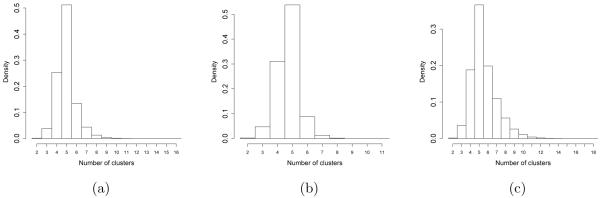
Posterior distribution of the number of clusters in the simulation of Section 5.3 (τ = 0.25). Case (a) corresponds to a Beta-GOS(α_n = n, β_n = 1), case (b) to a Beta-GOS(α_n = β_n = 1) and case (c) to a Dirichlet Process with parameter θ = 1.

Finally, we note that in our simulations, posterior inference for the Beta-GOS process seemed only minimally affected by the two different specifications of the parameters of the Beta weights. This consideration confirms the suggestion that using α_n = n + θ − 1, β_n = 1 represents a default choice in many applications, where there is no a priori information to guide parameter choice. In this case, θ can be chosen or estimated similarly as what is routinely done for mixtures of DPs. The Supplemental Materials contain additional results for several specifications of the model hyper-parameters, overall confirming the above remarks.

5.4 Fitting Hidden Semi-Markov Models

A third simulation study is designed to assess the robustness of the Beta-GOS framework to a mis-specification of a different nature. In many problems (e.g. change point detection), hidden Markov Models are used as computationally convenient substitutes for temporal processes that are known to be more complex than implied by first order Markovian dynamics. Here, we generate non-exchangeable sequences from a hidden semi-Markov process (HSMM; Ferguson, 1980; Yu, 2010) and study how the Beta-GOS process performs in fitting this type of data. Hidden semi-Markov processes are an extension of the popular hidden Markov model where the time spent in each state (state occupancy or sojourn time) is given by an explicit (discrete) distribution. A geometric state occupancy distribution characterizes ordinary hidden Markov models. Therefore, hidden semi-Markov process have also been referred to as “hidden Markov Models with explicit duration” (Mitchell et al., 1995; Dewar et al., 2012) or “variable-duration hidden Markov Models” (Rabiner, 1989).

We generate 1,000 datasets (1000 observations each) using a hidden semi-Markov process with four states and a negative binomial distribution for the state occupancy distribution. More specifically, we parametrize the negative binomial in terms of its mean and an ancillary parameter, which is directly related to the amount of overdispersion of the distribution (Hilbe, 2011; Airoldi et al., 2006). If the data are not overdispersed, the Negative Binomial reduces to the Poisson, and the ancillary parameter is zero. For the simulations presented here, we consider a NegBin(15, 0.15), which corresponds to assuming a large overdispersion (17.25). We also consider τ = 0.25 and τ = 0.5 in order to explore robustness to different levels of noise. We fit the data by means of a Beta-GOS model with Beta hyper-parameters defined by: a) α_n = n, β_n = 1; b) α_n = 5, β_n = 1; c) α_n = 1, β_n = 1. Based on Proposition 1, those choices correspond to assuming different clustering behaviors; in particular, different expected number of clusters a priori. We then compare the Beta-GOS with the fit resulting from hidden Markov models, assuming 3, 4 and 5 states, respectively. Results from the simulations are reported in Table 3, where the HMM was implemented using the R package “RHmm” (Taramasco and Bauer, 2012). Table 3 shows that the Beta-GOS is a viable alternative to HMM, as it can provide more accurate inference than a single hidden Markov model where the number of states is fixed a priori. As expected, higher levels of noise decrease the accuracy of the estimates, but the reduction affects the fit of the Beta-GOS and hidden Markov Models similarly. Furthermore, the fit obtained with the Beta-GOS appears quite robust to the different choices of the hyper-parameters. Figure 2 illustrates the clustering induced by the Beta-Gos and a 4-state HMM for a subset of the data generated in two specific simulation replicates. The middle column illustrates the allocation, respectively, from a Beta-Gos(α_n = 1, β_n = 1) (top) and a Beta-Gos(α_n = n, β_n = 1)(bottom), whereas column (c) illustrates the clustering attained by the HMM. Caution is necessary in order to avoid over-interpreting the results in the figure. Overall, the segmentation-plots suggest similarity in the allocations induced by the Beta-GOS and the HMM. In some instances, the Beta-GOS fit seems to allow shorter stretches of contiguous identical states, as illustrated in the top row of Figure 2. On the other hand, when data are characterized by elevated intra-claster variability, as in the bottom row of Figure 2, both the Beta-Gos and the HMM could fail to attain a fair representation of the true clustering structure of the data. Our practical experience suggests that the issue is more prominent for the “default” Beta-Gos(α_n = n, β_n = 1) than for the “informative” Beta-Gos(α_n = a, β_n = b) formulations. This is in accordance with the discussion in Section 3 and, in particular, with the consideration that a Beta-Gos(α_n = n, β_n = 1) should represent a long memory process where all previous observations are expected to contribute the same weight in (3). The Supplementary Materials contain results for a wider range of parameter settings, as well as different data generating mechanisms, confirming the results noted above.

Table 3.

Summary statistics for the simulation studies described in Section 5.4. The table compares the Beta-GOS and a hidden Markov model under different specifications of hyper-parameters. The data generating process assumes a hidden semi-Markov with state occupancy distribution NegBin(15, 0.15) and two levels of the sampling noise τ = 0.25 and τ = 0.5.

i) Data Generating Process: Hidden Semi Markov Model (HSMM) with 4 states and NegBin(15, 0.15)
Model Fitting Method	Beta-GOS			HMM
	αn = n; βn = 1	αn = 5; βn = 1	αn = 1; βn = 1	3 States	4 States	5 States
			τ = 0.25
Estimated Number of Clusters	3.89 ± 0.53	4.04 ± 0.59	4.09 ± 0.63	2.98 ± 0.13	3.94 ± 0.29	4.87 ± 0.55
Accuracy of Cluster Assignment	0.95 ± 0.10	0.97 ± 0.07	0.96 ± 0.08	0.72 ± 0.09	0.84 ± 0.13	0.90 ± 0.13
			τ = 0.5
Estimated Number of Clusters	3.69 ± 0.81	3.89 ± 0.96	4.06 ± 0.97	2.99 ± 0.12	3.96 ± 0.25	4.90 ± 0.48
Accuracy of Cluster Assignment	0.86 ± 0.14	0.90 ± 0.12	0.90 ± 0.12	0.71 ± 0.11	0.83 ± 0.12	0.88 ± 0.13

Figure 2.

Illustrative segmentation-type plots for the simulation study in Section 5.4. Column (a): subset of data for two replicates. Column (b) top: an example of allocation for a Beta-Gos(α_n = 1, β_n = 1) plotted vs the truth (black line); column (b) bottom considers a Beta-Gos(α_n = n, β_n = 1). Column (c) illustrates the fitting by a HMM with 4 states.

6. QUANTIFYING CHROMOSOMAL ABERRATIONS IN BREAST CANCER

We first apply the Beta-GOS to a classic dataset that has been used to link patterns of chromosomal aberrations to breast cancer pathophysiologies in the medical literature (Chin et al., 2006). The raw data measure genome copy number gains and losses over 145 primary breast tumor samples, across the 23 chromosomes, obtained using BAC array Comparative Genomic Hybridization (CGH). More precisely, the measurements consist of log₂ intensity ratios obtained from the comparison of cancer and normal female genomic DNA labeled with distinct fluorescent dyes and co-hybridized on a microarray in the presence of Cot-1 DNA to suppress unspecific hybridization of repeat sequences (see Redon et al., 2009). The analysis of array CGH data presents some challenges, because data are typically very noisy and spatially correlated. More specifically, copy numbers gains or losses at a region are often associated to an increased probability of gains and losses at a neighboring region. We use the Beta-GOS model developed in the previous Sections to analyze and cluster clones with similar level of amplification/deletion, for each breast tumor sample and each chromosome in the dataset. For array CGH data, it is typical to distinguish regions with a normal amount of chromosomal material, from regions with single copy loss (deletion), single copy gain and amplifications (multiple copy gains). Therefore, we present here the results of the analysis where the latent Beta hyper-parameters are set to α_n = 3 and β_n = 1, corresponding to E(K_n) = 4 states for large n (see Section 3). We have also considered α_n = n and β_n = 1, with no remarkable differences in the results. We complete the specification of model (6)–(7) with a vague base distribution, Normal(0, 10), and a vague inverse gamma distribution for τ centered around τ = 0.1. This choice of τ is motivated by the typical scale of the array CGH data and is in accordance with similar choices in the literature (see, for example Guha et al., 2008).

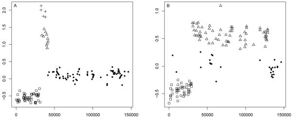
Figure 3 exemplifies the fit to chromosome 8 on two tumor samples. The model is able to identify regions of reduced copy number variation and high amplification. Note how contiguous clones tend to be clustered together, in a pattern typical of these chromosomal aberrations. Figure 4 replicates Figure 1 in Chin et al. (2006) and shows the frequencies of genome copy number gains and losses among all 145 samples plotted as a function of genome location. In order to identify a copy number aberration for this plot, for each chromosome and sample, at each iteration we consider the cluster with lowest absolute mean and order the other clusters accordingly. The lowest absolute mean is chosen to identify the copy neutral state. Following Guha et al. (2008) any other cluster is identified as a copy number gain or loss if its mean, say ${\widehat{\mathit{\mu }}}_{\mathrm{(}\mathit{j}\mathrm{)}}$, is farther than a specified threshold from the minimum absolute mean, say ${\widehat{\mathit{\mu }}}_{\mathrm{(}\mathrm{1}\mathrm{)}}$, i.e. if ${\widehat{\mathit{\mu }}}_{\mathrm{(}\mathit{j}\mathrm{)}}\mathrm{-}{\widehat{\mathit{\mu }}}_{\mathrm{(}\mathrm{1}\mathrm{)}}\mathrm{>}\mathit{\epsilon }$. We experimented with a range of choices of ε in the range [0.05, 0.15] and used ε = 0.1 for the current analysis. Furthermore, if the mean of a cluster is above the mean of all declared gains plus two standard deviations, all genes in that cluster are considered high level amplifications. We identify a clone with an aberration (or high level amplification) if it is such in more than 70% of the MCMC iterations; then, we compute the frequency of aberrations and high level amplifications among all 145 samples, which are reported, respectively, at the top and bottom of Figure 4. As expected, the clusters identified by the model tend to be localized in space all over the genome. This feature may be facilitated by the increasingly low reinforcement of far away clones embedded in the Beta-GOS, and corresponds to the understanding that clones that live at adjacent locations on a chromosome can be either amplified or deleted together due to the recombination process.

Figure 3.

Model fit overview: Array CGH gains and losses on chromosome 8 for two samples of breast tumors in the dataset in (Chin et al., 2006). Points with different shapes denote different clusters.

Figure 4.

A) Frequencies of genome copy number gains and losses plotted as a function of genomic location. B) Frequency of tumors showing high-level amplification. The dashed vertical lines separate the 23 chromosomes.

Finally, we considered some regions of chromosomes 8, 11, 17, and 20 that have been identified by Chin et al. (2006) and shown to correlate in their analysis to increased gene expression. We adapt the procedure described in Newton et al. (2004) to compute a region-based measure of the false discovery rate (FDR) and determine the q-values for neutral-state and aberration regions estimated in our analysis. The q-value is the FDR analogue of the p-value, as it measures the minimum FDR threshold at which we may determine that a region corresponds to significant copy number gains or losses (Storey, 2003; Storey et al., 2007). More specifically, after conducting a clone based test as described in the previous paragraph, we identify regions of interest by taking into account the strings of consecutive calls. These regions then constitute the units of the subsequent cluster based FDR analysis. Alternatively, the regions of interest could be pre-specified on the basis of the information available in the literature. The optimality of the type of procedures here described for cluster based FDR is discussed in Sun et. al, 2014. See also Heller et al., 2006, Müller et al., 2007 and Ji et al., 2008). In Table 4 we report the q-values from a set of candidate oncogenes in well-known regions of recurrent amplification (notably, 8p12, 8q24, 11q13-14, 12q13-14, 17q21-24, and 20q13). Our findings confirm the previous detections of chromosomal aberrations in the same locations.

Table 4.

False discovery rate analysis for clones with high-level amplification previously identified by Chin et al. (2006). The individual amplicons are reported together with the locations of the flanking clones on the array platform.

Amplicon	Flanking clone (left)	Flanking clone (right)	Kb start	Kb end	FDR q-value
8p11-12	RP11-258M15	RP11-73M19	33579	43001	0.021
8q24	RP11-65D17	RP11-94M13	127186	132829	0.021
11q13-14	CTD-2080I19	RP11-256P19	68482	71659	0.022
11q13-14	RP11-102M18	RP11-215H8	73337	78686	0.024
12q13-14	BAL12B2624	RP11-92P22	67191	74053	0.011
17q11-12	RP11-5808	RP11-87N6	34027	38681	0.017
17q21-24	RP11-234J24	RP11-84E24	45775	70598	0.017
20q13	RMC20B4135	RP11-278I13	51669	53455	0.021
20q13	GS-32I19	RP11-94A18	55630	59444	0.017

Next, we apply our methodology to the analysis of a modern large-scale CGH array dataset (Curtis et al., 2012). More specifically, here we consider one sample from the data published by Curtis et al. (2012). We fit the Beta-GOS model to the entire sequence of 969,700 probes matched to genomics locations using a priority queue on the Harvard Odyssey cluster. Model fit took about 24 hours. We also fit a Hidden Markov model and a Hidden semi-Markov model with Negative-Binomial run lengths times, both set to have three states (Yau et al., 2011), to the same sample. The parameters of both models were estimated using standard techniques (Rabiner, 1989; Guedon, 2003). The estimates for the Negative-Binomial run lengths, shared across states for simplicity, were r̂ = 10 and $\widehat{\mathit{\Pi }}\mathrm{\approx }\mathrm{0}\mathrm{.}\mathrm{2}\mathrm{5}$, leading to a mean run length of 30 probes with a standard deviation of 10.

For validation purposes, we accessed a list of 152 consensus genomic locations where chromosomal aberrations were found in Breast cancer tumor samples. This list is included in the data files associated with The Genome Cancer Atlas (TCGA) project, partly curated by the Broad Institute and hosted by the NIH. The 152 consensus genomic locations range in size from 5 to 49 probes. This list provides a list of locations, which have been reported as likely altered in terms of DNA content in a number of publications, using multiple types of datasets and analyses. Therefore, the list is independent of the specifics of any particular technique, and it can be used as a reference for evaluating the comparative performance of our Beta-GOS model with Hidden Markov models, and Hidden semi-Markov models. For each method, we declared a success at detecting a chromosomal aberration (either deletion or amplification) at any of the 152 consensus genomic locations if the method correctly labeled at least 80% of the probes associated with any given consensus genomic location. This choice was necessary since locations span multiple probes. According to this simple measure of performance, the Beta-GOS correctly labeled 133 locations (or 87.50%) of the 152 consensus genomic locations as having a chromosomal aberration, versus 94 locations (or 61.84%) using the Hidden Markov model, and 118 locations (or 77.63%) using the Hidden semi-Markov model. Of course, caution should be should be taken against over-interpreting the results of a single illustrative example. However, the results from the simulation studies and data analysis all concur to suggests that the Beta-GOS is a flexible model and that can be usefully employed in detecting chromosomal aberrations in array CGH data, since it can account for long range dependences in the sequence and achieve improved accuracy with respect to competing Hidden Markov Model based approaches.

7. CONCLUDING REMARKS

Starting from the characterization of species sampling sequences in terms of their predictive probability functions, we have considered predictive rules where the weights are functions of latent Beta random variables. The resulting Beta-GOS process defines a novel and probabilistically coherent Bayesian Nonparametric model for non-exchangeable data. We have discussed the clustering behavior of the Beta-GOS processes for some specifications of the latent Beta densities and illustrated their use as priors in a hierarchical model setting. Finally, we have analyzed the performance of this modeling framework by means of a set of simulation studies. The results outlined in Section 6 illustrate how the proposed Beta-GOS model can be a useful tool for the analysis of CGH array data. In medical applications, for instance, it might be used to complement tumor sub-type definition, or to suggest candidate genes for follow-up clinical studies. We expect our approach will be useful in other applications where Hidden Markov and semi-Markov model are currently considered as standard, e.g. in text segmentation and speech processing (e.g., Rabiner, 1989; Blei and Moreno, 2001; Chien and Furui, 2005; Ren et al., 2010; Yau and Holmes, 2013; Fox et al., 2014).

Recently, Teh et al. (2006a), Fox et al. (2011), and Yau et al. (2011) have developed flexible and effective hierarchical Bayesian nonparametric extensions of hidden Markov models that allow posterior inference over the number of states. The Beta-GOS model provides an alternative, non-exchangeable, Bayesian nonparametric formalism to model heterogeneity across non-exchangeable observations that are sequentially ordered, by enabling clustering in a number of unknown states. Since the Beta-GOS model does not rely on the estimation of a single transition matrix across time points, as in the HMM, we do not need to consider an explicit parameter to account for state persistence, as in Fox et al. (2011), or assume a distribution for the sojourn times as in HSMMs. Indeed, since the predictive weights depend on the sequence of observations itself, the Beta-GOS seems particularly convenient when the underlying generative process is non-stationary, e.g. as a possible alternative to more complicated non-homogeneous HMMs. Monteiro et al. (2011) discuss a similar issue in a product partition model framework and explicitly assume that the observations in a cluster have their distributions indexed by different parameters. Our approach is different, for example we do not need to explicitly model the dependence structure within the clusters.

Arguably, the major obstacle we can foresee in the wider applicability of this type of models relies in the specification of the prior hyper-parameters in the latent Beta distributions. Some specific suggestions have been provided in Section 3. However, in cases where there is not enough prior information to advise differently, our experience suggests that the default choice of the hyper-parameters outlined in Proposition 1(a) not only reduces the problem to the choice of a single parameter as it is usual in DP mixture models, but may also suffice for inferential purposes. Alternatively, one could assume a prior distribution on the parameters of the Beta latent variables and conduct posterior inference by means of MCMC methods, as briefly discussed in Section 4. Nevertheless, in specific applications the optimal modeling of the latent Beta densities requires further study and will be pursued elsewhere. In addition, the proposed approach inherits the general computational limitations of nonparametric Bayesian methods. For example, a full MCMC algorithm for posterior inference may be unfeasible for genomic sequences with several millions of reads. Scalable algorithms may facilitate fast inference in those settings (e.g., Colella et. al., 2007).

Finally, we believe that the flexibility of the latent specification and the possibility to tie the clustering implied by the Generalized Pólya Urn scheme directly to a set of latent random variables gives an opportunity to further modeling the complex relationships typical of heterogenous datasets. For example, further developments may substitute the general latent Beta specification with a probit/logistic specification, and define a Generalized Pólya Urn scheme in the aims of Rodriguez et al. (2010) that allows the clustering at each observation to be dependent on a set of (possibly sequentially recorded) covariates or curves. Similarly, we can imagine using multivariate Generalized Pólya Urn schemes of the sort we describe in this paper to model time dependent parameters in time series, which may be important to identify time-varying structures or regime changes at the base of phenomena like the so called financial contagion, i.e. the co-movement of asset prices across global markets after large shocks (see, for example, Liu et. al, 2012).

A. APPENDIX: DETAILS OF POSTERIOR MCMC SAMPLING FOR THE BETA-GOS MODEL

Here, we provide the details of the MCMC sampling algorithm described in Section 4.2 for the special case of a Normal sampling distribution and a Normal (or Normal-Inverse-Gamma) base measure.

A.1 Full conditionals for the Gibbs sampler

At each iteration of Gibbs sampler we sample from the full conditionals of C_n and W_n, for n = 1, … , N . Here we derive the analytical form of these distributions, for the Beta-GOS model specified in Section 5. Recall that the full conditional distribution for C_n is

$$\mathit{P}\mathrm{\left\{}{\mathit{C}}_{\mathit{n}}\mathrm{=}\mathit{i}\mathrm{\right|}{\mathit{C}}_{\mathrm{-}\mathit{n}}\mathrm{,}\mathrm{}\mathit{W}\mathrm{(}\mathit{N}\mathrm{)}\mathrm{,}\mathrm{}\mathit{Y}\mathrm{(}\mathit{N}\mathrm{)}\mathrm{,}\mathrm{}{\mathit{\tau }}^{\mathrm{2}}\mathrm{\}}\mathrm{\propto }\mathit{P}\mathrm{\{}\mathit{Y}\mathrm{(}\mathit{N}\mathrm{)}\mathrm{|}{\mathit{C}}_{\mathit{n}}\mathrm{=}\mathit{i}\mathrm{,}\mathrm{}{\mathit{C}}_{\mathrm{-}\mathit{n}}\mathrm{,}\mathrm{}\mathit{W}\mathrm{(}\mathit{N}\mathrm{)}\mathrm{,}\mathrm{}{\mathit{\tau }}^{\mathrm{2}}\mathrm{\}}\mathrm{\cdot }\mathit{P}\mathrm{\left\{}{\mathit{C}}_{\mathit{n}}\mathrm{=}\mathit{i}\mathrm{\right|}{\mathit{C}}_{\mathrm{-}\mathit{n}}\mathrm{,}\mathrm{}\mathit{W}\mathrm{(}\mathit{N}\mathrm{)}\mathrm{\}}$$

where the factor on the right is given by (8) and (3), and the left factor is obtained by integration,

$$\mathit{P}\left\{\mathit{Y}\mathrm{\left(}\mathit{N}\mathrm{\right)}\mathrm{|}{\mathit{C}}_{\mathit{n}}\mathrm{=}\mathit{i},{\mathit{C}}_{\mathrm{-}\mathit{n}},\mathit{W}\mathrm{\left(}\mathit{N}\mathrm{\right)},{\mathit{\tau }}^{\mathrm{2}}\right\}\mathrm{=}\mathit{P}\left\{\mathit{Y}\mathrm{\left(}\mathit{N}\mathrm{\right)}\mathrm{|}{\mathit{C}}_{\mathit{n}}\mathrm{=}\mathit{i},\mathrm{}{\mathit{C}}_{\mathrm{-}\mathit{n}},{\mathit{\tau }}^{\mathrm{2}}\right\}\mathrm{=}{\displaystyle \int }\mathit{P}\left\{\mathit{Y}\mathrm{\left(}\mathit{N}\mathrm{\right)},\mathit{\mu }\mathrm{|}{\mathit{C}}_{\mathit{n}}\mathrm{=}\mathit{i},{\mathit{C}}_{\mathrm{-}\mathit{n}},{\mathit{\tau }}^{\mathrm{2}}\right\}\mathit{d}\mathit{\mu }\mathrm{=}{\displaystyle \underset{\mathit{j}\mathrm{=}\mathrm{1}}{\overset{\mathit{J}}{\Pi }}{\int }_{\mathit{l}}\underset{\mathrm{\in }{\mathrm{\Pi }}_{\mathit{j}}}{\Pi }}\mathit{p}\mathrm{\left(}{\mathit{Y}}_{\mathit{l}}\mathrm{\right|}{\mathit{\mu }}_{\mathit{j}}^{\mathrm{*}}\mathrm{\left)}{\mathit{G}}_{\mathrm{0}}\mathrm{\right(}\mathit{d}{\mathit{\mu }}_{\mathit{j}}^{\mathrm{*}}\mathrm{)}\mathrm{\propto }{\displaystyle \underset{\mathit{j}\mathrm{=}\mathrm{1}}{\overset{\mathit{J}}{\Pi }}}\frac{\mathrm{1}}{\sqrt{\mathrm{2}\mathit{\pi }}}\frac{\mathrm{1}}{{\mathrm{\left(}\mathit{\tau }\mathrm{\right)}}^{\left|{\mathrm{\Pi }}_{\mathit{j}}\right|}}\exp \{\mathrm{-}\frac{{{\displaystyle \sum }}_{\mathit{l}\mathrm{\in }{\mathrm{\Pi }}_{\mathit{j}}}{\mathit{y}}_{\mathit{l}}^{\mathrm{2}}}{\mathrm{2}{\mathit{\tau }}^{\mathrm{2}}}\mathrm{-}\frac{{\mathit{\mu }}_{\mathrm{0}}^{\mathrm{2}}}{\mathrm{2}{\mathit{\sigma }}_{\mathrm{0}}^{\mathrm{2}}}\mathrm{+}\frac{\mathrm{1}}{\mathrm{2}}\frac{{\left(\frac{\mathit{\mu }\mathrm{0}}{{\mathit{\sigma }}_{\mathrm{0}}^{\mathrm{2}}}+{{\displaystyle \sum }}_{\mathit{l}\mathrm{\in }{\mathrm{\Pi }}_{\mathit{j}}}\frac{{\mathit{y}}_{\mathit{l}}}{{\mathit{\tau }}^{\mathrm{2}}}\right)}^{\mathrm{2}}}{\frac{\mathrm{1}}{{\mathit{\sigma }}_{\mathrm{0}}^{\mathrm{2}}}\mathrm{+}\frac{\mathrm{\left|}{\mathrm{\Pi }}_{\mathit{j}}\mathrm{\right|}}{{\mathit{\tau }}^{\mathrm{2}}}}\}\frac{\mathrm{1}}{\sqrt{\frac{\mathrm{\left|}{\mathrm{\Pi }}_{\mathit{j}}\mathrm{\right|}{\mathit{\sigma }}_{\mathrm{0}}^{\mathrm{2}}}{{\mathit{\tau }}^{\mathrm{2}}}\mathrm{+}\mathrm{1}}},$$

where Π_j is the set of indices of data points in cluster j, and J is the number of clusters at that iteration. Note that the latent reinforcements W(N) are used to define the cluster assignments through the data-pairing labels C(N). Conditionally on the data-pairing labels C(N), the data Y(N) is independent of the latent reinforcements W(N).

The full conditional for W_n, denoted by P(W_n|C(N), W_−n, Y(N)), is Beta distributed with updated parameters A_n, B_n, defined as in (8).

A.2 Inference on the cluster centroids of the Beta-GOS process

For the purpose of computational efficiency, it is generally preferable to sample the random partitions integrating out with respect to the parameters of the Beta-GOS process, as described in Section 4.2 and in Appendix A.1. If the sampling distribution and the base measure are conjugate, this usually results in improved mixing of the chain. However, in many cases, it may be required to draw inferences on the cluster centroids themselves. As usual with mixtures of DP, inference on the cluster centroids can be easily conducted (even ex-post) from the clustering configurations at each iteration. Therefore, we do not have to sample the centroids within each Gibbs iteration, but if the need be, we can easily resample them at the end of each iteration, or at the end of the sampler from the stored output.

A.3 Inference on the cluster and global variances

Let the variance of the sampling distribution be τ ². We assume τ ² ~ IGamma(a₀, b₀). The posterior distribution of the variance in each cluster j, is given by

$${\mathit{\tau }}_{\mathit{j}}^{\mathrm{2}}\mathrm{|}{\mathit{\mu }}_{\mathit{j}}^{\mathrm{*}}{\mathit{Y}}_{\mathit{i}}\mathit{i}\mathrm{\in }{\mathrm{\Pi }}_{\mathit{j}}\mathrm{~}\mathit{I}\mathit{G}\mathit{\alpha }\mathit{m}\mathit{m}\mathit{\alpha }\mathrm{(}{\mathit{\alpha }}_{\mathrm{0}}\mathrm{+}\frac{\mathrm{\left|}{\mathrm{\Pi }}_{\mathit{j}}\mathrm{\right|}}{\mathrm{2}}\mathrm{,}\mathrm{}{\mathit{b}}_{\mathrm{0}}\mathrm{+}\frac{\mathrm{1}}{\mathrm{2}}{{\displaystyle \sum }}_{\mathit{i}\mathrm{\in }{\mathrm{\Pi }}_{\mathit{j}}}\mathrm{(}{\mathit{Y}}_{\mathit{i}}\mathrm{-}{\mathit{\mu }}_{\mathit{j}}^{\mathrm{*}}\mathrm{)}\mathrm{2}\mathrm{)}$$

Note that, in case of need and for computational efficiency, we could use these also quantities to obtain a global estimate for the sampling variance at each iteration, in an MCMC-EM step, as ${\widehat{\mathit{\tau }}}^{\mathrm{2}}\mathrm{=}{{\displaystyle \sum }}_{\mathit{j}\mathrm{=}\mathrm{1}}^{\mathit{J}}\frac{\mathrm{(}\mathrm{\left|}{\mathrm{\Pi }}_{\mathit{j}}\mathrm{\right|}\mathrm{-}\mathrm{1}\mathrm{)}{\mathit{\tau }}_{\mathit{j}}^{\mathrm{2}}}{\mathit{N}\mathrm{-}\mathit{J}}$. This may turn useful, for example, for parallelization purposes, as in the simulations of Section 5.

A.4 Inference on the cluster means

In the normal-normal model described in Section 5, the posterior distribution of ${\mathit{\mu }}_{\mathit{j}}^{\mathrm{*}}$ given data Y_i in the j-th cluster can be evaluated at each iteration as

$$\mathit{P}\mathrm{(}{\mathit{\mu }}_{\mathit{j}}^{\mathrm{*}}\mathrm{|}{\mathit{\tau }}_{\mathit{j}}^{\mathrm{2}}\mathrm{,}\mathrm{}{\mathit{Y}}_{\mathit{i}}\mathrm{,}\mathrm{}\mathit{i}\mathrm{\in }{\mathrm{\pi }}_{\mathit{j}}\mathrm{)}\mathrm{~}\mathit{N}\mathrm{(}\frac{\frac{\mathit{\mu }\mathrm{0}}{{\mathit{\sigma }}_{\mathrm{0}}^{\mathrm{2}}}\mathrm{+}\frac{\mathrm{\left|}{\mathrm{\pi }}_{\mathit{j}}\mathrm{\right|}\stackrel{‒}{{\mathit{Y}}_{\mathit{j}}}}{{\mathit{\tau }}_{\mathit{j}}^{\mathrm{2}}}}{\frac{\mathrm{1}}{{\mathit{\sigma }}_{\mathrm{0}}^{\mathrm{2}}}\mathrm{+}\frac{\mathrm{\left|}{\mathrm{\Pi }}_{\mathit{j}}\mathrm{\right|}}{{\mathit{\tau }}_{\mathit{j}}^{\mathrm{2}}}}\mathrm{,}\mathrm{(}\frac{\mathrm{1}}{{\mathit{\sigma }}_{\mathrm{0}}^{\mathrm{2}}}\mathrm{+}\frac{\mathrm{\left|}{\mathrm{\Pi }}_{\mathit{j}}\mathrm{\right|}}{{\mathit{\tau }}_{\mathit{j}}^{\mathrm{2}}}\mathrm{)}\mathrm{-}\mathrm{1}\mathrm{)}$$

for j = 1, … , J , where Ȳ^j is the j-th cluster specific mean. Note that we have assumed a common sampling variance τ²; the modification of the previous formula to take into account a cluster specific variance is of course straightforward.

B. APPENDIX: DETAILS OF THE PROOFS AND ADDITIONAL THEORETICAL RESULTS

B.1 Generalized Ottawa Sequence and its moments

According to Bassetti et al. (2010) a sequence (X_n)_n≥1 of random variables taking values in a Polish space is a Generalized Ottawa Sequence if there exists a sequence (W_n)_n≥1 (of random variables) such that the following conditions are satisfied: (i) the law of X₁ is G₀; (ii) for n ≥ 1, X_n+1 and the subsequence (W_n+j)_j≥1 are conditionally independent given the filtration ƒ_n := σ(X₁, … , X_n, W₁, … , W_n); (iii) the predictive distribution of X_n+1 given ƒ_n is given by (3) where the r_n’s are strictly positive functions, r_n(W₁, … , W_n), of the vector of latent variables, such that

$${\mathit{r}}_{\mathit{n}}\mathrm{(}{\mathit{W}}_{\mathrm{1}}\mathrm{,}\mathrm{}\mathrm{\text{...}}\mathrm{,}\mathrm{}{\mathit{W}}_{\mathit{n}}\mathrm{)}\mathrm{\ge }{\mathit{r}}_{\mathit{n}\mathrm{+}\mathrm{1}}\mathrm{(}{\mathit{W}}_{\mathrm{1}}\mathrm{,}\mathrm{}\mathrm{\text{...}}\mathrm{,}\mathrm{}{\mathit{W}}_{\mathit{n}}\mathrm{,}\mathrm{}{\mathit{W}}_{\mathit{n}\mathrm{+}\mathrm{1}}\mathrm{),}$$ (A.1)

almost surely, with r₀ = 1, and the weights p_n,i = p_n,i(W₁, … , W_n) are

$${\mathit{p}}_{\mathit{n}\mathrm{,}\mathit{i}}\mathrm{=}\frac{{\mathit{r}}_{\mathit{n}}\mathrm{(}{\mathit{r}}_{\mathit{i}\mathrm{-}\mathrm{1}}\mathrm{-}{\mathit{r}}_{\mathit{i}}\mathrm{)}}{{\mathit{r}}_{\mathit{i}\mathrm{-}\mathrm{1}}{\mathit{r}}_{\mathit{i}}}\mathit{i}\mathrm{=}\mathrm{1,}\mathrm{\text{...,}}\mathit{n}$$ (A.2)

The predictive distribution (3)-(4) corresponds to choice r_n(W₁, … , W_n) = ${\mathit{r}}_{\mathit{n}}\mathrm{(}{\mathit{W}}_{\mathrm{1}}\mathrm{,}\mathrm{}\mathrm{\text{...}}\mathrm{,}\mathrm{}{\mathit{W}}_{\mathit{n}}\mathrm{)}\mathrm{=}{{\displaystyle \Pi }}_{\mathit{i}\mathrm{=}\mathrm{1}}^{\mathit{n}}{\mathit{W}}_{\mathit{i}}$ where (W_n)_n≥1 is a sequence of independent random variables.

We conclude this Section by providing a general result for the k-th moment and for the moment generating function of the length K_n of a GOS. Suppose that the sequence (X_n)_n≥1 is a GOS, with G₀ diffuse, and let U_j = K_j − K_j−1 with K₀ = 0. Then, ${\mathit{K}}_{\mathit{n}}\mathrm{=}{{\displaystyle \sum }}_{\mathit{j}\mathrm{=}\mathrm{1}}^{\mathit{n}}{\mathit{U}}_{\mathit{j}}$ and the joint distribution of U₁, … , U_n conditionally on r₁, … , r_n−1, is

$\mathit{P}\mathrm{\{}{\mathit{U}}_{\mathrm{1}}\mathrm{=}\mathrm{1}\mathrm{,}\mathrm{}\mathrm{\text{...}}\mathrm{,}\mathrm{}{\mathit{U}}_{\mathit{n}}\mathrm{=}{\mathit{e}}_{\mathit{n}}\mathrm{|}{\mathit{r}}_{\mathrm{1}}\mathrm{,}\mathrm{}\mathrm{\text{...}}\mathrm{,}\mathrm{}{\mathit{r}}_{\mathit{n}\mathrm{-}\mathrm{1}}\mathrm{\}}\mathrm{=}\underset{\mathit{i}\mathrm{=}\mathrm{2}}{\overset{\mathit{n}}{{\displaystyle \Pi }}}{\mathit{r}}_{\mathit{i}\mathrm{-}\mathrm{1}}^{{\mathit{e}}_{\mathit{i}}}\mathrm{(}\mathrm{1}\mathrm{-}{\mathit{r}}_{\mathit{i}\mathrm{-}\mathrm{1}}\mathrm{)}\mathrm{1}\mathrm{-}{\mathit{e}}_{\mathit{i,}}$

for every vector (e₂, … , e_n) in {0, 1}ⁿ⁻¹, since P (U₁ = 1) = 1 by definition. Since K₁ = U₁ = 1, it follows that, for every k ≥ 1,

$$\mathit{P}\mathrm{\{}{\mathit{K}}_{\mathit{n}\mathrm{+}\mathrm{1}}\mathrm{=}\mathit{k}\mathrm{+}\mathrm{1}\mathrm{\}}\mathrm{=}\mathit{P}\mathrm{\left\{}{\displaystyle \sum }_{\mathit{j}\mathrm{=}\mathrm{2}}^{\mathit{n}\mathrm{+}\mathrm{1}}{\mathit{U}}_{\mathit{j}}\mathrm{=}\mathit{k}\mathrm{\right\}}\mathrm{=}{{\displaystyle \sum }}_{\underset{‒}{e}}\mathit{E}\mathrm{[}\underset{\mathit{i}\mathrm{=}\mathrm{1}}{\overset{\mathit{n}}{{\displaystyle \Pi }}}{\mathit{r}}_{\mathit{i}\mathrm{-}\mathrm{1}}^{{\mathit{e}}_{\mathit{i}}}\mathrm{(}\mathrm{1}\mathrm{-}{\mathit{r}}_{\mathit{i}\mathrm{-}\mathrm{1}}\mathrm{)}\mathrm{1}\mathrm{-}{\mathit{e}}_{\mathit{i}}\mathrm{]}$$

where the summation is extended over all sequences e = (e₁, … , e_n) in {0, 1}ⁿ such that ${{\displaystyle \sum }}_{\mathit{i}\mathrm{=}\mathrm{1}}^{\mathit{n}}{\mathit{e}}_{\mathit{i}}\mathrm{=}\mathit{k}$. Moreover, for every k ≥ 1 and n ≥ 2, it is easy to see that

$$\mathit{E}\mathrm{[}\mathrm{(}{\mathit{K}}_{\mathit{n}\mathrm{+}\mathrm{1}}\mathrm{-}\mathrm{1}\mathrm{)}\mathit{k}\mathrm{]}\mathrm{=}\mathit{E}\mathrm{\left[}\mathrm{(}{\displaystyle \sum }_{\mathit{j}\mathrm{=}\mathrm{2}}^{\mathit{n}\mathrm{+}\mathrm{1}}{\mathit{U}}_{\mathit{j}}\mathrm{)}\mathit{k}\mathrm{\right]}\mathrm{=}{\displaystyle \sum }_{\mathit{m}\mathrm{=}\mathrm{1}}^{\mathit{k}\mathrm{^}\mathit{n}}\mathit{m}\mathrm{!}\mathit{S}\mathrm{(}\mathit{k}\mathrm{,}\mathrm{}\mathit{m}\mathrm{)}{\mathit{\phi }}_{\mathit{n}\mathrm{,}\mathit{m}}$$ (A.3)

where k Λ n = min(k, n),

$${\mathit{\phi }}_{\mathit{n}\mathrm{,}\mathit{m}}\mathrm{:}\mathrm{=}{{\displaystyle \sum }}_{\mathrm{1}\mathrm{\le }{\mathit{l}}_{\mathrm{1}}\mathrm{<}{\mathit{l}}_{\mathrm{2}}\mathrm{<}\mathrm{\cdot }\mathrm{\cdot }\mathrm{<}{\mathit{l}}_{\mathit{m}}\mathrm{\le }\mathit{n}}\mathrm{.}\mathit{E}\mathrm{[}{\mathit{r}}_{{\mathit{l}}_{\mathrm{1}}}\mathrm{\text{...}}{\mathit{r}}_{{\mathit{l}}_{\mathit{m}}}\mathrm{].}$$ (A.4)

and $\mathit{S}\mathrm{(}\mathit{k}\mathrm{,}\mathrm{}\mathit{m}\mathrm{)}\mathrm{:}\mathrm{=}\frac{\mathit{k}\mathrm{!}}{\mathit{m}\mathrm{!}}{{\displaystyle \sum }}_{\mathrm{\{}{\mathit{n}}_{\mathit{i}}\mathrm{>}\mathrm{0}\mathrm{:}{\mathrm{\Sigma }}_{\mathit{i}\mathrm{=}\mathrm{1}}^{\mathit{m}}{\mathit{n}}_{\mathit{i}}\mathrm{=}\mathit{k}\mathrm{\}}}\frac{\mathrm{1}}{{\mathit{n}}_{\mathrm{1}}\mathrm{!}\mathrm{\text{...}}{\mathit{n}}_{\mathit{m}}\mathrm{!}}$ is the Stirling number of second kind. Hence, E[(K_n+1 − 1)^k] depends recursively on functions φ_n−1,m, m = 1, … , k. It may be interesting to note that, using the well known relation between factorial moments and ordinary moments (see, e.g., Example 2.3 in Charalambides, 2005), from (A.3) one gets, for any m ≤ n,

$$\mathit{E}\mathrm{[}\mathrm{(}{\mathit{K}}_{\mathit{n}\mathrm{+}\mathrm{1}}\mathrm{-}\mathrm{1}\mathrm{)}\mathrm{(}\mathit{m}\mathrm{)}\mathrm{]}\mathrm{=}\mathit{m}\mathrm{!}{\mathit{\phi }}_{\mathit{n}\mathrm{,}\mathit{m}}$$ (A.5)

where (t)_(m) = t(t − 1) … (t − m + 1) is the falling factorial. Moreover, since

$${{\displaystyle \sum }}_{\mathit{k}\mathrm{\ge }\mathit{m}}\mathrm{(}\mathrm{-}\mathit{t}\mathrm{)}\mathit{k}\frac{\mathit{S}\mathrm{(}\mathit{k}\mathrm{,}\mathit{m}\mathrm{)}}{\mathit{k}\mathrm{!}}\mathrm{=}\frac{\mathrm{(}\mathit{e}\mathrm{-}\mathit{t}\mathrm{-}\mathrm{1}\mathrm{)}\mathit{m}}{\mathit{m}\mathrm{!}}$$

see e.g. Thm. 2.3 in Charalambides (2005), it follows that the moment generating function of K_n+1 is given by

$${\mathit{M}}_{\mathit{n}\mathrm{+}\mathrm{1}}\mathrm{(}\mathit{t}\mathrm{)}\mathrm{:}\mathrm{=}\mathit{E}\mathrm{\left[}{\mathit{e}}^{\mathrm{-}\mathit{t}{\mathit{K}}_{\mathit{n}\mathrm{+}\mathrm{1}}}\mathrm{\right]}\mathrm{=}{\mathit{e}}^{\mathrm{-}\mathit{t}}\mathit{E}\mathrm{\left[}{\mathit{e}}^{\mathrm{-}\mathit{t}\mathrm{(}{\mathit{K}}_{\mathit{n}\mathrm{+}\mathrm{1}}\mathrm{-}\mathrm{1}\mathrm{)}}\mathrm{\right]}\mathrm{=}{\mathit{e}}^{\mathrm{-}\mathit{t}}{{\displaystyle \sum }}_{\mathit{k}\mathrm{\ge }\mathrm{0}}\frac{\mathrm{(}\mathrm{-}\mathit{t}\mathrm{)}\mathit{k}}{\mathit{k}\mathrm{!}}\mathit{E}\mathrm{[}\mathrm{(}{\mathit{K}}_{\mathit{n}\mathrm{+}\mathrm{1}}\mathrm{-}\mathrm{1}\mathrm{)}\mathit{k}\mathrm{]}\mathrm{=}{\mathit{e}}^{\mathrm{-}\mathit{t}}\mathrm{+}{\mathit{e}}^{\mathrm{-}\mathit{t}}{{\displaystyle \sum }}_{\mathit{k}\mathrm{\ge }\mathrm{1}}{\displaystyle \sum }_{\mathit{m}\mathrm{=}\mathrm{1}}^{\mathit{k}\mathrm{^}\mathit{n}}\frac{\mathrm{(}\mathrm{-}\mathit{t}\mathrm{)}\mathit{k}\mathit{m}\mathrm{!}}{\mathit{k}\mathrm{!}}\mathit{S}\mathrm{(}\mathit{k}\mathrm{,}\mathrm{}\mathit{m}\mathrm{)}{\mathit{\phi }}_{\mathit{n}\mathrm{,}\mathit{m}}\mathrm{=}{\mathit{e}}^{\mathrm{-}\mathit{t}}\mathrm{+}{\mathit{e}}^{\mathrm{-}\mathit{t}}{\displaystyle \sum }_{\mathit{m}\mathrm{=}\mathrm{1}}^{\mathit{n}}\mathit{m}\mathrm{!}{\mathit{\phi }}_{\mathit{n}\mathrm{,}\mathit{m}}{{\displaystyle \sum }}_{\mathit{k}\mathrm{\ge }\mathit{m}}\frac{\mathrm{(}\mathrm{-}\mathit{t}\mathrm{)}\mathit{k}}{\mathit{k}\mathrm{!}}\mathit{S}\mathrm{(}\mathit{k}\mathrm{,}\mathrm{}\mathit{m}\mathrm{)}\mathrm{=}{\mathit{e}}^{\mathrm{-}\mathit{t}}{\displaystyle \sum }_{\mathit{m}\mathrm{=}\mathrm{0}}^{\mathit{n}}\mathrm{(}{\mathit{e}}^{\mathrm{-}\mathit{t}}\mathrm{-}\mathrm{1}\mathrm{)}\mathit{m}{\mathit{\phi }}_{\mathit{n}\mathrm{,}\mathit{m}}$$ (A.6)

with φ_n,0 := 1.

B.2 Proof of Proposition 1

If we consider equation (A.4) with (W_i)_i≥1 independent random variables taking values in [0, 1], then

$${\mathit{\phi }}_{\mathit{n}\mathrm{,}\mathit{m}}\mathrm{=}{{\displaystyle \sum }}_{\mathrm{1}\mathrm{\le }{\mathit{l}}_{\mathrm{1}}\mathrm{<}{\mathit{l}}_{\mathrm{2}}\mathrm{<}\mathrm{\cdot }\mathrm{\cdot }\mathrm{<}{\mathit{l}}_{\mathit{m}}\mathrm{\le }\mathit{n}}\mathrm{.}\underset{\mathit{j}\mathrm{=}\mathrm{1}}{\overset{\mathit{m}}{{\displaystyle \Pi }}}\underset{\mathit{i}\mathrm{=}{\mathit{l}}_{\mathit{j}\mathrm{-}\mathrm{1}}\mathrm{+}\mathrm{1}}{\overset{{\mathit{l}}_{\mathit{j}}}{{\displaystyle \Pi }}}\mathit{E}\mathrm{\left[}{\mathit{W}}_{\mathit{i}}^{\mathit{m}\mathrm{+}\mathrm{1}\mathrm{-}\mathit{j}}\mathrm{\right]}$$ (A.7)

where l₀ := 0. We need some preliminary results.

Lemma 2. If W_i ~ Beta(i + θ − 1, 1), for given θ > 0, then

$${\mathit{\phi }}_{\mathit{n}\mathrm{,}\mathit{m}}\mathrm{=}\frac{\mathrm{\Gamma }\mathrm{(}\mathit{\theta }\mathrm{+}\mathit{m}\mathrm{)}}{\mathrm{\Gamma }\mathrm{(}\mathit{\theta }\mathrm{)}}{\displaystyle \sum }_{{\mathit{j}}_{\mathrm{1}}\mathrm{=}\mathit{m}}^{\mathit{n}}{\displaystyle \sum }_{{\mathit{j}}_{\mathrm{2}}\mathrm{=}\mathit{m}\mathit{j}}^{{\mathit{j}}_{\mathrm{1}}}{\displaystyle \sum }_{{\mathrm{3}}^{\mathrm{=}\mathit{m}}}^{{\mathit{j}}_{\mathrm{2}}}\mathrm{\text{...}}{\displaystyle \sum }_{{\mathit{j}}_{\mathit{m}}\mathrm{=}\mathit{m}}^{{\mathit{j}}_{\mathit{m}\mathrm{-}\mathrm{1}}}\frac{\mathrm{1}}{\mathrm{(}{\mathit{j}}_{\mathrm{1}}\mathrm{+}\mathit{\theta }\mathrm{)}\mathrm{(}{\mathit{j}}_{\mathrm{2}}\mathrm{+}\mathit{\theta }\mathrm{)}\mathrm{\text{...}}\mathrm{(}{\mathit{j}}_{\mathit{m}}\mathrm{+}\mathit{\theta }\mathrm{)}}$$ (A.8)

In particular, as n goes to +∞,

$$\mathit{E}\mathrm{\left[}{\mathit{K}}_{\mathit{n}}^{\mathit{k}}\mathrm{\right]}\mathrm{=}\frac{\mathrm{\Gamma }\mathrm{(}\mathit{\theta }\mathrm{+}\mathit{k}\mathrm{)}}{\mathrm{\Gamma }\mathrm{(}\mathit{\theta }\mathrm{)}}{\log }^{\mathit{k}}\mathrm{(}\mathit{n}\mathrm{)}\mathrm{[}\mathrm{1}\mathrm{+}\mathit{o}\mathrm{(}\mathrm{1}\mathrm{)}\mathrm{].}$$ (A.9)

Let us start by proving (A.8). First, note that since W_i is a Beta(i + θ − 1, 1) random variable then, for 1 ≤ j ≤ m, $\mathit{E}\mathrm{\left[}{\mathit{W}}_{\mathit{i}}^{\mathit{m}\mathrm{+}\mathrm{1}\mathrm{-}\mathit{j}}\mathrm{\right]}\mathrm{=}\frac{\mathit{i}\mathrm{+}\mathit{\theta }\mathrm{-}\mathrm{1}}{\mathit{i}\mathrm{+}\mathit{\theta }\mathrm{+}\mathit{m}\mathrm{-}\mathit{j}}$. Hence, by (A.7),

$${\mathit{\phi }}_{\mathit{n}\mathrm{,}\mathit{m}}\mathrm{=}{{\displaystyle \sum }}_{\mathrm{1}\mathrm{\le }{\mathit{l}}_{\mathrm{1}}\mathrm{<}{\mathit{l}}_{\mathrm{2}}\mathrm{<}\mathrm{\cdot }\mathrm{\cdot }\mathrm{<}{\mathit{l}}_{\mathit{m}}\mathrm{\le }\mathit{n}}\mathrm{.}\underset{\mathit{j}\mathrm{=}\mathrm{1}}{\overset{\mathit{m}}{{\displaystyle \Pi }}}\underset{\mathit{i}\mathrm{=}{\mathit{l}}_{\mathit{j}\mathrm{-}\mathrm{1}}\mathrm{+}\mathrm{1}}{\overset{{\mathit{l}}_{\mathit{j}}}{{\displaystyle \Pi }}}\frac{\mathit{i}\mathrm{+}\mathit{\theta }\mathrm{-}\mathrm{1}}{\mathit{i}\mathrm{+}\mathit{\theta }\mathrm{+}\mathit{m}\mathrm{-}\mathit{j}}$$ (A.10)

which, after some algebra, returns (A.8). In order to prove the second part of Lemma 2 we need to introduce additional notation. For θ > 0, k ≥ 1, m ≥ 2 and n ≥ k, set

$${\mathrm{\Psi }}_{\mathit{k}\mathrm{,}\mathit{\theta }}\mathrm{(}\mathit{n}\mathrm{,}\mathrm{}\mathit{m}\mathrm{)}\mathrm{:}\mathrm{=}{\displaystyle \sum }_{{\mathit{j}}_{\mathrm{1}}\mathrm{=}\mathit{k}}^{\mathit{n}}{\displaystyle \sum }_{{\mathit{j}}_{\mathrm{2}}\mathrm{=}\mathit{k}}^{{\mathit{j}}_{\mathrm{1}}}{\displaystyle \sum }_{{\mathit{j}}_{\mathrm{3}}\mathrm{=}\mathit{k}}^{{\mathit{j}}_{\mathrm{2...}}}{\displaystyle \sum }_{{\mathit{j}}_{\mathit{m}}\mathrm{=}\mathit{k}}^{{\mathit{j}}_{\mathit{m}\mathrm{-}\mathrm{1}}}\frac{\mathit{m}\mathrm{!}}{\mathrm{(}{\mathit{j}}_{\mathrm{1}}\mathrm{+}\mathit{\theta }\mathrm{)}\mathrm{(}{\mathit{j}}_{\mathrm{2}}\mathrm{+}\mathit{\theta }\mathrm{)}\mathrm{\text{...}}\mathrm{(}{\mathit{j}}_{\mathit{m}}\mathrm{+}\mathit{\theta }\mathrm{),}}{\mathrm{\Psi }}_{\mathit{k}\mathrm{,}\mathit{\theta }}\mathrm{(}\mathit{n}\mathrm{,}\mathrm{}\mathrm{1}\mathrm{)}\mathrm{:}\mathrm{=}{\displaystyle \sum }_{{\mathit{j}}_{\mathrm{1}}\mathrm{=}\mathit{k}}^{\mathit{n}}\frac{\mathrm{1}}{\mathrm{(}{\mathit{j}}_{\mathrm{1}}\mathrm{+}\mathit{\theta }\mathrm{)}}$$

Note that m!φ_n,m = Ψ_m,θ(n, m)Γ(θ + m)/Γ(θ). For all k ≥ 1, m ≥ 1 and n ≥ k, set Q_k,θ (m, n) := Ψ_k,θ (n, m) − log^m(n + θ). Now formula (A.9) in Lemma 2 follows easily from (A.3) and the next result.

Lemma 3. For θ > 0, k ≥ 1 and m ≥ 1, there is a constant C_k,θ (m) such that

$$\mathrm{|}{\mathit{Q}}_{\mathit{k}\mathrm{,}\mathit{\theta }}\mathrm{(}\mathit{m}\mathrm{,}\mathrm{}\mathit{n}\mathrm{)}\mathrm{|}\mathrm{\le }{\mathit{C}}_{\mathit{k}\mathrm{,}\mathit{\theta }}\mathrm{(}\mathit{m}\mathrm{)}{\log }^{\mathit{m}\mathrm{-}\mathrm{1}}\mathrm{(}\mathit{n}\mathrm{}\mathrm{+}\mathit{\theta }\mathrm{)\; for\; every}\mathit{n}\mathrm{\ge }\mathit{k}$$ (A.11)

Let k ≥ 1 and θ > 0. For m ≥ 1 and n ≥ k set

$${\mathit{S}}_{\mathit{k}\mathrm{,}\mathit{\theta }}\mathrm{(}\mathit{m}\mathrm{,}\mathrm{}\mathit{n}\mathrm{)}\mathrm{;}\mathrm{=}{\displaystyle \sum }_{\mathit{j}\mathrm{=}\mathit{k}}^{\mathit{n}}\frac{\mathit{m}{\log }^{\mathit{m}\mathrm{-}\mathrm{1}}\mathrm{(}\mathit{j}\mathrm{+}\mathit{\theta }\mathrm{)}}{\mathit{j}\mathrm{+}\mathit{\theta ,}\mathrm{and}}{\mathit{R}}_{\mathit{k}\mathrm{,}\mathit{\theta }}\mathrm{(}\mathit{m}\mathrm{,}\mathrm{}\mathit{n}\mathrm{)}\mathrm{:}\mathrm{=}{\mathit{S}}_{\mathit{k}\mathrm{,}\mathit{\theta }}\mathrm{(}\mathit{m}\mathrm{,}\mathrm{}\mathit{n}\mathrm{)}\mathrm{-}{\log }^{\mathit{m}}\mathrm{(}\mathit{n}\mathrm{}\mathrm{+}\mathit{\theta }\mathrm{)}\mathrm{=}{\displaystyle \sum }_{\mathit{j}\mathrm{=}\mathit{k}}^{\mathit{n}}\frac{\mathit{m}{\log }^{\mathit{m}\mathrm{-}\mathrm{1}}\mathrm{(}\mathit{j}\mathrm{+}\mathit{\theta }\mathrm{)}}{\mathit{j}\mathrm{+}\mathit{\theta }}\mathrm{-}{\log }^{\mathit{m}}\mathrm{(}\mathit{n}\mathrm{}\mathrm{+}\mathit{\theta }\mathrm{)}$$ 12

We claim that, for any m ≥ 1, there is a constant ${\mathit{C}}_{\mathit{m}}^{\mathrm{*}}\mathrm{=}{\mathit{C}}_{\mathit{m}\mathrm{,}\mathit{\theta }\mathrm{,}\mathit{k}}^{\mathrm{*}}$ such that

$$\mathrm{|}{\mathit{R}}_{\mathit{k}\mathrm{,}\mathit{\theta }}\mathrm{(}\mathit{m}\mathrm{,}\mathrm{}\mathit{n}\mathrm{)}\mathrm{|}\mathrm{\le }{\mathit{C}}_{\mathit{m}}^{\mathrm{*}\mathrm{for\; all}}\mathit{n}\mathrm{\ge }\mathit{k}$$ (A.13)

Now observe that Ψ_k,θ (n, 1) = S_k,θ (1, n). Hence, (A.13) proves (A.11) for m = 1 and every k ≥ 1 and θ > 0. By induction suppose that (A.11) is true for m = 1, … , M − 1. Note that, for m ≥ 2,

$${\mathrm{\Psi }}_{\mathit{k}\mathrm{,}\mathit{\theta }}\mathrm{(}\mathit{n}\mathrm{,}\mathrm{}\mathit{m}\mathrm{)}\mathrm{=}{\displaystyle \sum }_{{\mathit{j}}_{\mathrm{1}}\mathrm{=}\mathit{k}}^{\mathit{n}}\frac{\mathit{m}}{{\mathit{j}}_{\mathrm{1}}\mathrm{+}\mathit{\theta }}{\mathrm{\Psi }}_{\mathit{k}\mathrm{,}\mathit{\theta }}\mathrm{(}{\mathit{j}}_{\mathrm{1}}\mathrm{,}\mathrm{}\mathit{m}\mathrm{-}\mathrm{1}\mathrm{)}$$

hence, by induction hypothesis, for every θ > 0, k ≥ 1 and n ≥ k,

$$\mathrm{\Psi }\mathit{k}\mathrm{,}\mathit{\theta }\mathrm{(}\mathit{n}\mathrm{,}\mathrm{}\mathit{M}\mathrm{)}\mathrm{=}{\displaystyle \sum }_{{\mathit{j}}_{\mathrm{1}}\mathrm{=}\mathit{k}}^{\mathit{n}}\frac{\mathit{M}}{{\mathit{j}}_{\mathrm{1}}\mathrm{+}\mathit{\theta }}\mathrm{[}{\log }^{\mathit{M}\mathrm{-}\mathrm{1}}\mathrm{(}{\mathit{j}}_{\mathrm{1}}\mathrm{+}\mathit{\theta }\mathrm{)}\mathrm{+}{\mathit{Q}}_{\mathit{k}\mathrm{,}\mathit{\theta }}\mathrm{(}\mathit{M}\mathrm{-}\mathrm{1}\mathrm{,}\mathrm{}{\mathit{j}}_{\mathrm{1}}\mathrm{)}\mathrm{].}$$

Using (A.12) one gets

$${\mathrm{\Psi }}_{\mathit{k}\mathrm{,}\mathit{\theta }}\mathrm{(}\mathit{n}\mathrm{,}\mathrm{}\mathit{M}\mathrm{)}\mathrm{=}{\log }^{\mathit{M}}\mathrm{(}\mathit{n}\mathrm{}\mathrm{+}\mathit{\theta }\mathrm{)}\mathrm{+}{\mathit{R}}_{\mathit{k}\mathrm{,}\mathit{\theta }}\mathrm{(}\mathit{M}\mathrm{,}\mathrm{}\mathit{n}\mathrm{)}\mathrm{+}{\displaystyle \sum }_{{\mathit{j}}_{\mathrm{1}}\mathrm{=}\mathit{k}}^{\mathit{n}}\frac{\mathit{M}}{{\mathit{j}}_{\mathrm{1}}\mathrm{+}\mathit{\theta }}{\mathit{Q}}_{\mathit{k}\mathrm{,}\mathit{\theta }}\mathrm{(}\mathit{M}\mathrm{-}\mathrm{1}\mathrm{,}\mathrm{}{\mathit{j}}_{\mathrm{1}}\mathrm{).}$$

Hence, using (A.13) and the induction hypothesis, one can write

$$\left|{\mathit{Q}}_{\mathit{k}\mathrm{,}\mathit{\theta }}\mathrm{(}\mathit{M}\mathrm{,}\mathit{n}\mathrm{)}\right|\mathrm{\le }\left|{\mathit{R}}_{\mathit{k}\mathrm{,}\mathit{\theta }}\mathrm{(}\mathit{M}\mathrm{,}\mathit{n}\mathrm{)}\right|\mathrm{+}{\displaystyle \sum }_{{\mathit{j}}_{\mathrm{1}}\mathrm{=}\mathit{k}}^{\mathit{n}}\frac{\mathit{M}}{{\mathit{j}}_{\mathrm{1}}\mathrm{+}\mathit{\theta }}\left|{\mathit{Q}}_{\mathit{k}\mathrm{,}\mathit{\theta }}\mathrm{(}\mathit{M}\mathrm{-}\mathrm{1}\mathrm{,}{\mathit{j}}_{\mathrm{1}}\mathrm{)}\right|\mathrm{\le }{\mathit{C}}_{\mathit{M}\mathrm{,}\mathit{\theta }\mathrm{,}\mathit{k}}^{\mathrm{*}}\mathrm{+}\frac{\mathit{M}{\mathit{C}}_{\mathit{k}\mathrm{,}\mathit{\theta }}\mathrm{(}\mathit{M}\mathrm{-}\mathrm{1}\mathrm{)}}{\mathit{M}\mathrm{-}\mathrm{1}}{\displaystyle \sum }_{{\mathit{j}}_{\mathrm{1}}\mathrm{=}\mathit{k}}^{\mathit{n}}\frac{\mathit{M}\mathrm{-}\mathrm{1}}{{\mathit{j}}_{\mathrm{1}}\mathrm{+}\mathit{\theta }}{\log }^{\mathit{M}\mathrm{-}\mathrm{2}}\mathrm{(}{\mathit{j}}_{\mathrm{1}}\mathrm{+}\mathit{\theta }\mathrm{)}\mathrm{\le }{\mathit{C}}_{\mathit{M}\mathrm{,}\mathit{\theta }\mathrm{,}\mathit{k}}^{\mathrm{*}}\mathrm{+}\frac{\mathit{M}{\mathit{C}}_{\mathit{k}\mathrm{,}\mathit{\theta }}\mathrm{(}\mathit{M}\mathrm{-}\mathrm{1}\mathrm{)}}{\mathit{M}\mathrm{-}\mathrm{1}}\mathrm{\left[}{\log }^{\mathit{M}\mathrm{-}\mathrm{1}}\mathrm{(}\mathit{n}\mathrm{+}\mathit{\theta }\mathrm{)}\mathrm{+}\mathrm{\right|}{\mathit{R}}_{\mathit{k}\mathrm{,}\mathit{\theta }}\mathrm{(}\mathit{M}\mathrm{-}\mathrm{1}\mathrm{,}\mathit{n}\mathrm{)}\mathrm{\left|}\mathrm{\right]}\mathrm{\le }{\mathit{C}}_{\mathit{M}\mathrm{,}\mathit{\theta }\mathrm{,}\mathit{k}}^{\mathrm{*}}\mathrm{+}\frac{\mathit{M}{\mathit{C}}_{\mathit{k}\mathrm{,}\mathit{\theta }}\mathrm{(}\mathit{M}\mathrm{-}\mathrm{1}\mathrm{)}}{\mathit{M}\mathrm{-}\mathrm{1}}\mathrm{\left[}{\log }^{\mathit{M}\mathrm{-}\mathrm{1}}\mathrm{(}\mathit{n}\mathrm{+}\mathit{\theta }\mathrm{)}\mathrm{+}{\mathit{C}}_{\mathit{M}\mathrm{-}\mathrm{1}\mathrm{,}\mathit{\theta }\mathrm{,}\mathit{k}}^{\mathrm{*}}\mathrm{\right]}$$

which proves (A.11) for m = M . To complete the proof let us prove (A.13). Observe that $\mathit{x}\mathrm{\mapsto }\frac{{\log }^{\mathit{m}\mathrm{-}\mathrm{1}}\mathrm{(}\mathit{x}\mathrm{+}\mathit{\theta }\mathrm{)}}{\mathit{x}\mathrm{+}\mathit{\theta }}$ is a non-increasing function on [x₀, +∞) for a suitable x₀ = x₀(k, θ, m). Assume, without real loss of generality, that k ≥ x₀ + 1. Note that, in this case,

$${{\displaystyle \int }}_{\mathit{k}}^{\mathit{n}\mathrm{+}\mathrm{1}}\frac{\mathit{m}{\log }^{\mathit{m}\mathrm{-}\mathrm{1}}\mathrm{(}\mathit{x}\mathrm{+}\mathit{\theta }\mathrm{)}}{\mathit{x}\mathrm{+}\mathit{\theta }}\mathit{d}\mathit{x}\mathrm{\le }{\mathit{S}}_{\mathit{k}\mathrm{,}\mathit{\theta }}\mathrm{(}\mathit{m}\mathrm{,}\mathrm{}\mathit{n}\mathrm{)}\mathrm{\le }{{\displaystyle \int }}_{\mathit{k}\mathrm{-}\mathrm{1}}^{\mathit{n}}\frac{\mathit{m}{\log }^{\mathit{m}\mathrm{-}\mathrm{1}}\mathrm{(}\mathit{x}\mathrm{+}\mathit{\theta }\mathrm{)}}{\mathit{x}\mathrm{+}\mathit{\theta }}\mathit{d}\mathit{x}$$

Hence,

$${\log }^{\mathit{m}}\mathrm{(}\mathit{n}\mathrm{}\mathrm{+}\mathrm{1}\mathrm{+}\mathit{\theta }\mathrm{)}\mathrm{-}{\log }^{\mathit{m}}\mathrm{(}\mathit{k}\mathrm{+}\mathit{\theta }\mathrm{)}\mathrm{\le }{\mathit{S}}_{\mathit{k}\mathrm{,}\mathit{\theta }}\mathrm{(}\mathit{m}\mathrm{,}\mathrm{}\mathit{n}\mathrm{)}\mathrm{\le }{\log }^{\mathit{m}}\mathrm{(}\mathit{n}\mathrm{}\mathrm{+}\mathit{\theta }\mathrm{)}\mathrm{-}{\log }^{\mathit{m}}\mathrm{(}\mathit{k}\mathrm{-}\mathrm{1}\mathrm{+}\mathit{\theta }\mathrm{),}$$

which gives

$${\log }^{\mathit{m}}\mathrm{(}\mathit{n}\mathrm{}\mathrm{+}\mathit{\theta }\mathrm{)}\mathrm{-}{\log }^{\mathit{m}}\mathrm{(}\mathit{k}\mathrm{+}\mathit{\theta }\mathrm{)}\mathrm{\le }{\mathit{S}}_{\mathit{k}\mathrm{,}\mathit{\theta }}\mathrm{(}\mathit{m}\mathrm{,}\mathrm{}\mathit{n}\mathrm{)}\mathrm{\le }{\log }^{\mathit{m}}\mathrm{(}\mathit{n}\mathrm{}\mathrm{+}\mathit{\theta }\mathrm{)}$$

and then

$$\mathrm{|}{\mathit{S}}_{\mathit{k}\mathrm{,}\mathit{\theta }}\mathrm{(}\mathit{m}\mathrm{,}\mathrm{}\mathit{n}\mathrm{)}\mathrm{-}{\log }^{\mathit{m}}\mathrm{(}\mathit{n}\mathrm{}\mathrm{+}\mathit{\theta }\mathrm{)}\mathrm{|}\mathrm{\le }{\log }^{\mathit{m}}\mathrm{(}\mathit{k}\mathrm{+}\mathit{\theta }\mathrm{)}$$

Proof of Proposition 1 (a). It follows immediately from (A.9) and a classical result concerning the convergence in distribution when the moments converge. Indeed,$\mathit{E}\mathrm{\left[}\mathrm{(}\frac{{\mathit{K}}_{\mathit{n}}}{\log \mathit{n}}\mathrm{)}\mathit{k}\mathrm{\right]}$ converges to $\frac{\mathrm{\Gamma }\mathrm{(}\mathit{\theta }\mathrm{+}\mathit{k}\mathrm{)}}{\mathrm{\Gamma }\mathrm{(}\mathit{\theta }\mathrm{)}}$ that is the k-th moment of a Γ(θ, 1) random variable.

Proof of Proposition 1 (b). The first part of the statement of Proposition 1(b) follows from Proposition 2.1 in Bassetti et al. (2010) if one shows that $\mathit{E}\mathrm{\left[}{{\displaystyle \sum }}_{\mathit{i}\mathrm{=}\mathrm{1}}^{\mathrm{\infty }}{\mathit{r}}_{\mathit{i}}\mathrm{\right]}\mathrm{<}\mathrm{\infty }$ . For α_n = a and β_n = b one gets E[r_n] = aⁿ/(a + b)ⁿ and the thesis follows. When α_n = n + θ − 1 and β_n = β, as explained in Section 3, E[r_n] ~ n^−β and the thesis follows since β > 1. It remains to prove the assertion concerning the moment generating function and the factorial moments of K_∞.

If α_n = a and β_n = b, (A.7) becomes

$${\mathit{\phi }}_{\mathit{n}\mathrm{,}\mathit{m}}\mathrm{=}{\displaystyle \sum }{\displaystyle \Pi }\mathrm{(}\mathit{E}\mathit{m}\mathrm{\left[}{\mathit{W}}_{\mathrm{1}}^{\mathit{m}\mathrm{+}\mathrm{1}\mathrm{-}\mathit{j}}\mathrm{\right]}\mathrm{)}{\mathit{l}}_{\mathit{j}}\mathrm{-}{\mathit{l}}_{\mathit{j}\mathrm{-}\mathrm{1,}}\mathrm{1}\mathrm{\le }{\mathit{l}}_{\mathrm{1}}\mathrm{<}{\mathit{l}}_{\mathrm{2}}\mathrm{<}\mathrm{\text{...}}\mathrm{<}{\mathit{l}}_{\mathit{m}}\mathrm{\le }\mathit{n}\mathit{j}\mathrm{=}\mathrm{1}{\displaystyle \sum }{\displaystyle \Pi }\mathrm{(}\stackrel{\mathit{m}}{{\displaystyle \Pi }}{\mathit{\gamma }}_{\mathit{i}}\mathrm{)}{\mathit{l}}_{\mathit{j}}\mathrm{-}{\mathit{l}}_{\mathit{j}\mathrm{-}\mathrm{1}}\mathit{m}\mathrm{+}\mathrm{1}\mathrm{-}\mathit{j}\mathrm{1}\mathrm{\le }{\mathit{l}}_{\mathrm{1}}\mathrm{<}{\mathit{l}}_{\mathrm{2}}\mathrm{<}\mathrm{\text{...}}\mathrm{<}{\mathit{l}}_{\mathit{m}}\mathrm{\le }\mathit{n}\mathit{j}\mathrm{=}\mathrm{1}\mathit{i}\mathrm{=}\mathrm{1}$$

since $\mathit{E}\mathrm{\left[}{\mathit{W}}_{\mathrm{1}}^{\mathit{m}}\mathrm{\right]}\mathrm{=}{{\displaystyle \Pi }}_{\mathit{i}\mathrm{=}\mathrm{1}}^{\mathit{m}}{\mathit{\gamma }}_{\mathit{i\; for}}{\mathit{\gamma }}_{\mathit{i}}\mathrm{=}\mathrm{(}\mathit{\alpha }\mathrm{+}\mathit{i}\mathrm{-}\mathrm{1}\mathrm{)}\mathrm{/}\mathrm{(}\mathit{\alpha }\mathrm{+}\mathit{b}\mathrm{+}\mathit{i}\mathrm{-}\mathrm{1}\mathrm{)}$. Taking the limit for n →+∞, we get

$${\lim }_{\mathit{n}}{\mathit{\phi }}_{\mathit{n}\mathrm{,}\mathit{m}}\mathrm{=}{{\displaystyle \sum }}_{\mathrm{1}\mathrm{\le }{\mathit{l}}_{\mathrm{1}}\mathrm{<}{\mathit{l}}_{\mathrm{2}}\mathrm{<}\mathrm{<}{\mathit{l}}_{\mathit{m}}}\mathrm{\text{...}}\underset{\mathit{j}\mathrm{=}\mathrm{1}}{\overset{\mathit{m}}{{\displaystyle \Pi }}}\mathrm{(}\underset{\mathit{i}\mathrm{=}\mathrm{1}}{\overset{\mathit{m}\mathrm{+}\mathrm{1}\mathrm{-}\mathit{j}}{{\displaystyle \Pi }}}{\mathit{\gamma }}_{\mathit{i}}\mathrm{)}{\mathit{l}}_{\mathit{j}}\mathrm{-}{\mathit{l}}_{\mathit{j}\mathrm{-}\mathrm{1}}\mathrm{=}{{\displaystyle \sum }}_{{\mathit{k}}_{\mathrm{1}}\mathrm{\ge }\mathrm{1}}{{\displaystyle \sum }}_{{\mathit{k}}_{\mathrm{2}}\mathrm{\ge }\mathrm{1.\; .\; .}}{{\displaystyle \sum }}_{{\mathit{k}}_{\mathit{m}}\mathrm{\ge }\mathrm{1}}\underset{\mathit{j}\mathrm{=}\mathrm{1}}{\overset{\mathit{m}}{{\displaystyle \Pi }}}\mathrm{(}\underset{\mathit{i}\mathrm{=}\mathrm{1}}{\overset{\mathit{m}\mathrm{+}\mathrm{1}\mathrm{-}\mathit{j}}{{\displaystyle \Pi }}}{\mathit{\gamma }}_{\mathit{i}}\mathrm{)}{\mathit{k}}_{\mathit{j}}\mathrm{=}\underset{\mathit{j}\mathrm{=}\mathrm{1}}{\overset{\mathit{m}}{{\displaystyle \Pi }}}{{\displaystyle \sum }}_{{\mathit{k}}_{\mathit{j}}\mathrm{\ge }\mathrm{1}}\mathrm{(}\underset{\mathit{i}\mathrm{=}\mathrm{1}}{\overset{\mathit{m}\mathrm{+}\mathrm{1}\mathrm{-}\mathit{j}}{{\displaystyle \Pi }}}{\mathit{\Gamma }}_{\mathit{i}}\mathrm{)}{\mathit{k}}_{\mathit{j}}\mathrm{=}\underset{\mathit{j}\mathrm{=}\mathrm{1}}{\overset{\mathit{m}}{{\displaystyle \Pi }}}\frac{{\mathit{\gamma }}_{\mathrm{1}}\mathrm{\text{...}}{\mathit{\gamma }}_{\mathit{j}}}{\mathrm{1}\mathrm{-}{\mathit{\gamma }}_{\mathrm{1}}\mathrm{\text{...}}{\mathit{\gamma }}_{\mathit{j}}}$$

and then

$${\lim }_{\mathit{n}}{\mathit{\phi }}_{\mathit{n}\mathrm{,}\mathit{m}}\mathrm{=}\underset{\mathit{j}\mathrm{=}\mathrm{1}}{\overset{\mathit{m}}{{\displaystyle \Pi }}}\frac{\mathrm{(}\mathit{\alpha }\mathrm{)}\mathrm{(}\mathit{j}\mathrm{)}}{\mathrm{(}\mathit{\alpha }\mathrm{+}\mathit{b}\mathrm{)}\mathrm{(}\mathit{j}\mathrm{)}\mathrm{-}\mathrm{(}\mathit{\alpha }\mathrm{)}\mathrm{(}\mathit{j}\mathrm{)}}$$

where (t)^(j) = t(t + 1) … (t + j − 1) is the rising factorial. Combining this fact with (A.6) it follows that, in this case,

$$\mathit{E}\mathrm{\left[}{\mathit{e}}^{\mathrm{-}\mathit{t}{\mathit{K}}_{\mathrm{\infty }}}\mathrm{\right]}\mathrm{=}{\mathit{e}}^{\mathrm{-}\mathit{t}}{{\displaystyle \sum }}_{\mathit{m}\mathrm{\ge }\mathrm{0}}\mathrm{(}{\mathit{e}}^{\mathrm{-}\mathit{t}}\mathrm{-}\mathrm{1}\mathrm{)}\mathit{m}\underset{\mathit{j}\mathrm{=}\mathrm{1}}{\overset{\mathit{m}}{{\displaystyle \Pi }}}\frac{\mathrm{(}\mathit{\alpha }\mathrm{)}\mathrm{(}\mathit{j}\mathrm{)}}{\mathrm{(}\mathit{\alpha }\mathrm{+}\mathit{b}\mathrm{)}\mathrm{(}\mathit{j}\mathrm{)}\mathrm{-}\mathrm{(}\mathit{\alpha }\mathrm{)}\mathrm{(}\mathit{j}\mathrm{)}}$$

In addition (A.3)-(A.5) give

$$\mathit{E}\mathrm{\left[}\frac{\mathrm{(}{\mathit{K}}_{\mathrm{\infty }}\mathrm{-}\mathrm{1}\mathrm{)}\mathit{m}}{\mathit{m}\mathrm{!}}\mathrm{\right]}\mathrm{=}\underset{\mathit{j}\mathrm{=}\mathrm{1}}{\overset{\mathit{m}}{{\displaystyle \Pi }}}\frac{\mathrm{(}\mathit{\alpha }\mathrm{)}\mathrm{(}\mathit{j}\mathrm{)}}{\mathrm{(}\mathit{\alpha }\mathrm{+}\mathit{b}\mathrm{)}\mathrm{(}\mathit{j}\mathrm{)}\mathrm{-}\mathrm{(}\mathit{\alpha }\mathrm{)}\mathrm{(}\mathit{j}\mathrm{),}}\mathit{E}\mathrm{[}\mathrm{(}{\mathit{K}}_{\mathrm{\infty }}\mathrm{-}\mathrm{1}\mathrm{)}\mathit{k}\mathrm{]}\mathrm{=}{\displaystyle \sum }_{\mathit{m}\mathrm{=}\mathrm{1}}^{\mathit{k}}\mathit{m}\mathrm{!}\mathit{S}\mathrm{(}\mathit{k}\mathrm{,}\mathrm{}\mathit{m}\mathrm{)}\underset{\mathit{j}\mathrm{=}\mathrm{1}}{\overset{\mathit{m}}{{\displaystyle \Pi }}}\frac{\mathrm{(}\mathit{\alpha }\mathrm{)}\mathrm{(}\mathit{j}\mathrm{)}}{\mathrm{(}\mathit{\alpha }\mathrm{+}\mathit{b}\mathrm{)}\mathrm{(}\mathit{j}\mathrm{)}\mathrm{-}\mathrm{(}\mathit{\alpha }\mathrm{)}\mathrm{(}\mathit{j}\mathrm{)}}$$

B.3 Conditionally identity in distribution of the Beta-GOS hierarchical model

Proposition 4. The sequence (Y_n)_n defined by formula (6)-(7) is conditionally identically distributed with respect to the filtration ${\mathsf{H}}_{\mathit{n}}\mathrm{=}\mathit{\sigma }\mathrm{(}\mathit{Y}\mathrm{(}\mathit{n}\mathrm{)}\mathrm{,}\mathrm{}\mathit{W}\mathrm{(}\mathit{n}\mathrm{)}\mathrm{,}\mathrm{}\mathit{\mu }\mathrm{(}\mathit{n}\mathrm{)}\mathrm{)}$ = σ(Y (n), W (n), μ(n)).

Proof. Let ${\mathsf{H}}_{\mathit{n}}\mathrm{=}\mathit{\sigma }\mathrm{(}\mathit{W}\mathrm{(}\mathit{n}\mathrm{)}\mathrm{,}\mathrm{}\mathit{\mu }\mathrm{(}\mathit{n}\mathrm{)}\mathrm{,}\mathrm{}\mathit{Y}\mathrm{(}\mathit{n}\mathrm{)}\mathrm{)}$. We have to prove that for every real, bounded and measurable function g

$$\mathit{E}\mathrm{(}\mathit{g}\mathrm{(}{\mathit{Y}}_{\mathit{n}\mathrm{+}\mathit{j}}\mathrm{)}\mathrm{\left|}{\mathsf{H}}_{\mathit{n}}\mathrm{)}\mathrm{=}\mathit{E}\mathrm{(}\mathit{g}\mathrm{(}{\mathit{Y}}_{\mathit{n}\mathrm{+}\mathrm{1}}\mathrm{)}\mathrm{\right|}{\mathsf{H}}_{\mathit{n}}\mathrm{)}$$ (A.14)

Now, for every j > 0

$$\mathsf{L}\mathrm{(}{\mathit{Y}}_{\mathit{n}\mathrm{+}\mathit{j}}\mathrm{|}{\mathsf{H}}_{\mathit{n}}\mathrm{,}\mathrm{}{\mathit{\mu }}_{\mathit{n}\mathrm{+}\mathit{j}}\mathrm{)}\mathrm{=}\mathsf{L}\mathrm{(}{\mathit{Y}}_{\mathit{n}\mathrm{+}\mathit{j}}\mathrm{|}{\mathit{\mu }}_{\mathit{n}\mathrm{+}\mathit{j}}\mathrm{)}\mathrm{=}\mathit{p}\mathrm{(}\mathrm{\cdot }\mathrm{|}{\mathit{\mu }}_{\mathit{n}\mathrm{+}\mathit{j}}\mathrm{)}$$ (A.15)

and for every j and n

$$\mathsf{L}\mathrm{(}{\mathit{\mu }}_{\mathit{n}\mathrm{+}\mathit{j}}\mathrm{\left|}{\mathsf{H}}_{\mathit{n}}\mathrm{)}\mathrm{=}\mathsf{L}\mathrm{(}{\mathit{\mu }}_{\mathit{n}\mathrm{+}\mathit{j}}\mathrm{\right|}{\mathsf{G}}_{\mathit{n}}\mathrm{)}$$ (A.16)

As already recalled, (μ_n)_n is CID with respect to ${\mathsf{G}}_{\mathit{n}}\mathrm{=}\mathit{\sigma }\mathrm{(}\mathit{W}\mathrm{(}\mathit{n}\mathrm{)}\mathrm{,}\mathrm{}\mathit{\mu }\mathrm{(}\mathit{n}\mathrm{)}\mathrm{)}$ = σ(W (n), μ(n)). This means that for every real, bounded and measurable function f

$$\mathit{E}\mathrm{(}\mathit{f}\mathrm{(}{\mathit{\mu }}_{\mathit{n}\mathrm{+}\mathit{j}}\mathrm{)}\mathrm{\left|}{\mathsf{G}}_{\mathit{n}}\mathrm{)}\mathrm{=}\mathit{E}\mathrm{(}\mathit{f}\mathrm{(}{\mathit{\mu }}_{\mathit{n}\mathrm{+}\mathrm{1}}\mathrm{)}\mathrm{\right|}{\mathsf{G}}_{\mathit{n}}\mathrm{)}$$ (A.17)

for all j ≥ 1, see Berti et al. (2004). Thanks to (A.16), equality (A.17) also holds with respect the sigma-field ${\mathsf{H}}_{\mathit{n}}$. Indeed,

$\mathit{E}\mathrm{(}\mathit{f}\mathrm{(}{\mathit{\mu }}_{\mathit{n}\mathrm{+}\mathit{j}}\mathrm{)}\mathrm{\left|}{\mathsf{H}}_{\mathit{n}}\mathrm{)}\mathrm{=}\mathit{E}\mathrm{(}\mathit{f}\mathrm{(}{\mathit{\mu }}_{\mathit{n}\mathrm{+}\mathit{j}}\mathrm{)}\mathrm{\right|}{\mathsf{G}}_{\mathit{n}}\mathrm{)}\mathrm{=}\mathit{E}\mathrm{(}\mathit{f}\mathrm{(}{\mathit{\mu }}_{\mathit{n}\mathrm{+}\mathrm{1}}\mathrm{)}\mathrm{\left|}{\mathsf{G}}_{\mathit{n}}\mathrm{)}\mathrm{=}\mathit{E}\mathrm{(}\mathit{f}\mathrm{(}{\mathit{\mu }}_{\mathit{n}\mathrm{+}\mathrm{1}}\mathrm{)}\mathrm{\right|}{\mathsf{H}}_{\mathit{n}}\mathrm{)}$

(A.15) implies that

$$\mathit{E}\mathrm{(}\mathit{g}\mathrm{(}{\mathit{Y}}_{\mathit{n}\mathrm{+}\mathit{j}}\mathrm{)}\mathrm{|}{\mathsf{H}}_{\mathit{n}}\mathrm{,}\mathrm{}{\mathit{\mu }}_{\mathit{n}\mathrm{+}\mathit{j}}\mathrm{)}\mathrm{=}\mathit{E}\mathrm{(}\mathit{g}\mathrm{(}{\mathit{Y}}_{\mathit{n}\mathrm{+}\mathit{j}}\mathrm{)}\mathrm{|}{\mathit{\mu }}_{\mathit{n}\mathrm{+}\mathit{j}}\mathrm{)}\mathrm{=}{\displaystyle \int }\mathit{g}\mathrm{(}\mathit{y}\mathrm{)}\mathit{p}\mathrm{(}\mathit{d}\mathit{y}\mathrm{|}{\mathit{\mu }}_{\mathit{n}\mathrm{+}\mathit{j}}\mathrm{)}$$ (A.18)

(A.17) and (A.18) allow to prove the thesis. Indeed,

$$\mathit{E}\mathrm{(}\mathit{g}\mathrm{(}{\mathit{Y}}_{\mathit{n}\mathrm{+}\mathit{j}}\mathrm{)}\mathrm{\left|}{\mathsf{H}}_{\mathit{n}}\mathrm{)}\mathrm{=}\mathit{E}\mathrm{(}\mathit{E}\mathrm{(}\mathit{g}\mathrm{(}{\mathit{Y}}_{\mathit{n}\mathrm{+}\mathit{j}}\mathrm{)}\mathrm{\right|}{\mathsf{H}}_{\mathit{n}}\mathrm{,}\mathrm{}{\mathit{\mu }}_{\mathit{n}\mathrm{+}\mathit{j}}\mathrm{\left|}{\mathsf{H}}_{\mathit{n}}\mathrm{)}\mathrm{=}\mathit{E}\mathrm{(}{\displaystyle \int }\mathit{g}\mathrm{(}\mathit{y}\mathrm{)}\mathit{p}\mathrm{(}\mathit{d}\mathit{y}\mathrm{\right|}{\mathit{\mu }}_{\mathit{n}\mathrm{+}\mathit{j}}\mathrm{)}\mathrm{\left|}{\mathsf{H}}_{\mathit{n}}\mathrm{)}\mathrm{=}\mathit{E}\mathrm{(}{\displaystyle \int }\mathit{g}\mathrm{(}\mathit{y}\mathrm{)}\mathit{p}\mathrm{(}\mathit{d}\mathit{y}\mathrm{\right|}{\mathit{\mu }}_{\mathit{n}\mathrm{+}\mathrm{1}}\mathrm{)}\mathrm{\left|}{\mathsf{H}}_{\mathit{n}}\mathrm{)}\mathrm{=}\mathit{E}\mathrm{(}\mathit{E}\mathrm{(}\mathit{g}\mathrm{(}{\mathit{Y}}_{\mathit{n}\mathrm{+}\mathrm{1}}\mathrm{)}\mathrm{\right|}{\mathsf{H}}_{\mathit{n}}\mathrm{,}\mathrm{}{\mathit{\mu }}_{\mathit{n}\mathrm{+}\mathrm{1}}\mathrm{\left|}{\mathsf{H}}_{\mathit{n}}\mathrm{)}\mathrm{=}\mathit{E}\mathrm{(}\mathit{g}\mathrm{(}{\mathit{Y}}_{\mathit{n}\mathrm{+}\mathrm{1}}\mathrm{)}\mathrm{\right|}{\mathsf{H}}_{\mathit{n}}\mathrm{)}$$

References

- Airoldi EM, Anderson A, Fienberg SE, Skinner KK. Who wrote Ronald Reagan’s radio addresses? Bayesian Analysis. 2006;1:289–320. [Google Scholar]
- Aoki M. Journal of Economic Dynamics and Control. 1. Vol. 32. Elsevier; 2008. Thermodynamic limits of macroeconomic or financial models: One-and two-parameter Poisson-Dirichlet models; pp. 66–84. [Google Scholar]
- Baladandayuthapani V, Ji Y, Nieto-Barajas LE, Morris JS. Bayesian random segmentation models to identify shared copy number aberrations for array CGH data. Journal of the American Statistical Association. 2010;105:1358–1375. doi: 10.1198/jasa.2010.ap09250. [DOI] [PMC free article] [PubMed] [Google Scholar]
- Bassetti F, Crimaldi I, Leisen F. Conditionally identically distributed species sampling sequences. Adv. in Appl. Probab. 2010;42:433–459. [Google Scholar]
- Berti P, Pratelli L, Rigo P. Limit Theorems for a Class of Identically Distributed Random Variables. Ann. Probab. 2004;32:2029–2052. [Google Scholar]
- Blackwell D, MacQueen JB. Ferguson distributions via Pólya urn schemes. Ann. Statist. 1973;1:353–355. [Google Scholar]
- Blei D, Frazier P. Distance dependent Chinese restaurant processes. Journal of Machine Learning Reseach. 2011;12:2461–2488. [Google Scholar]
- Blei DM, Moreno P. Topic segmentation with an aspect Hidden Markov Model; Proceedings of the 24th annual international ACM SIGIR conference; 2001. pp. 343–348. [Google Scholar]
- Cardin N, Holmes C, The Wellcome Trust Case Control Consortium. Donnelly P, Marchini J. Bayesian Hierarchical Mixture Modeling to Assign Copy Number from a Targeted CNV Array. Genetic Epidemiology. 2011;35:536–548. doi: 10.1002/gepi.20604. [DOI] [PMC free article] [PubMed] [Google Scholar]
- Charalambides CA. Combinatorial methods in discrete distributions. Wiley-Interscience, John Wiley & Sons; Hoboken, NJ: 2005. Wiley Series in Probability and Statistics. [Google Scholar]
- Chin K, DeVries S, Fridlyand J, Spellman PT, Roydasgupta R, Kuo WL, Lapuk A, Neve RM, Qian Z, Ryder T, Chen F, Feiler H, Tokuyasu T, Kingsley C, Dairkee S, Meng Z, Chew K, Pinkel D, Jain A, Ljung BM, Esserman L, Albertson DG, Waldman FM, Gray JW. Genomic and transcriptional aberrations linked to breast cancer pathophysiologies. Cancer Cell. 2006;10(6):529–541. doi: 10.1016/j.ccr.2006.10.009. [DOI] [PubMed] [Google Scholar]
- Chien JT, Furui S. Predictive hidden Markov model selection for speech recognition. IEEE Transactions on Speech and Audio Processing. 2005;13:377–387. [Google Scholar]
- Colella S, Yau C, Taylor JM, Mirza G, Butler H, Clouston P, Basset AS, Seller A, Holmes CC, Ragoussis J. QuantiSNP: an Object Bayes Hidden-Markov Model to detect and accurately map copy number variation using SNP genotyping data. Nucleic Acids Research. 2007;35:2013–2025. doi: 10.1093/nar/gkm076. [DOI] [PMC free article] [PubMed] [Google Scholar]
- Curtis C, Shah SP, Chin S-F, Turashvili G, Rueda OM, Dunning MJ, Speed D, Lynch AG, Samarajiwa S, Yuan Y, Gräf S, Ha G, Haffari G, Bashashati A, Russell R, McKinney S, METABRIC Group. Langer¿d A, Green A, Provenzano E, Wishart G, Pinder S, Watson P, Markowetz F, Murphy L, Ellis I, Purushotham A, B¿rresen-Dale A-L, Brenton JD, Tavar’e S, Caldas C, Aparicio S. The genomic and transcriptomic architecture of 2,000 breast tumours re-veals novel subgroups. Nature. 2012;486(7403):346–352. doi: 10.1038/nature10983. [DOI] [PMC free article] [PubMed] [Google Scholar]
- Dahl DB. Sequentially-Allocated Merge-Split Sampler for Conjugate and Nonconjugate Dirichlet Process Mixture Models. Technical Report. 2005.
- Dahl DB, Day R, Tsai JW. Distance-Based Probability Distribution on Set Partitions with Applications to Protein Structure Prediction. Technical Report. 2008.
- DeSantis SM, Houseman EA, Coull BA, Louis DN, Mohapatra G, Betensky RA. A Latent Class Model with Hidden Markov Dependence for Array CGH Data. Biometrics. 2009;65(4):1296–1305. doi: 10.1111/j.1541-0420.2009.01226.x. [DOI] [PMC free article] [PubMed] [Google Scholar]
- Dewar M, Wiggins C, Wood F. Inference in Hidden Markov Models with Explicit State Duration Distributions. Signal Processing Letters, IEEE. 19(4):235–238. [Google Scholar]
- Du L, Chen M, Lucas J, Carin L. Sticky Hidden Markov Modeling of Comparative Genomic Hybridization. IEEE Transactions on Signal Processing. 2010;58(10):5353–5368. [Google Scholar]
- Escobar M, West M. Bayesian Density Estimation and Inference Using Mixtures. Journal of the American Statistical Association. 1995;90:577–588. [Google Scholar]
- Ferguson JD. Variable duration models for speech; Proceedings of the Symposium on the Applications of Hidden Markov Models to Text and Speech; 1980. pp. 143–179. [Google Scholar]
- Fortini S, Ladelli L, Regazzini E. Exchangeability, predictive distributions and parametric models. Sankhya. 2000;62(1):86–109. Ser. A. [Google Scholar]
- Fox EB, Sudderth EB, Jordan MI, Willsky AS. A sticky HDP-HMM with application to speaker diarization. Annals of Applied Statistics. 2011;5(2A):1020–1056. [Google Scholar]
- Fox EB, Hughes MC, Sudderth EB, Jordan MI. Joint modeling of multiple time series via the Beta process with application to motion capture segmentation. Annals of Applied Statistics. 2014 To appear. [Google Scholar]
- Griffiths TL, Sanborn AN, Canini KR, Navarro DJ. Categorization as nonparametric Bayesian density estimation. In: Oaksford M, Chater N, editors. The Probabilistic Mind: Prospects for Rational Models of Cognition. Oxford University Press; Oxford: 2007. [Google Scholar]
- Guedon Y. Estimating hidden semi-Markov chains from discrete sequences. Journal of Computational and Graphical Statistics. 2011;12(3):604–639. [Google Scholar]
- Guha S, Li Y, Neuberg D. Bayesian Hidden Markov Modeling of Array CGH Data. Journal of the American Statistical Association. 2008;103:485–497. doi: 10.1198/016214507000000923. [DOI] [PMC free article] [PubMed] [Google Scholar]
- Guha S. Posterior Simulation in Countable Mixture Models for Large Datasets. Journal of the American Statistical Association. 2010;105(490):775–786. [Google Scholar]
- Hansen B, Pitman J. Prediction rules for exchangeable sequences related to species sampling. Statist. Probab. Lett. 2000;46:251–256. [Google Scholar]
- Heller R, Stanley D, Yekutieli D, Rubin N, Benjamini Y. Cluster-based analysis of fmri data. Neuroimage. 2006;33:599–608. doi: 10.1016/j.neuroimage.2006.04.233. [DOI] [PubMed] [Google Scholar]
- Hjort NL, Holmes C, Müller P, Walker SG. Bayesian Nonparametrics. Cambridge University Press; 2010. [Google Scholar]
- Hilbe JM. Negative Binomial Regression. Cambridge University Press; 2011. [Google Scholar]
- Ishwaran H, Zarepour M. Random probability measures via Pólya sequences: revisiting the Blackwell-MacQueen urn scheme. 2003 http://arxiv.org/abs/math/0309041.
- Jain S, Neal RM. Splitting and Merging Components of a Nonconjugate Dirichlet Process Mixture Model. Bayesian Analysis. 2007;3:445–472. [Google Scholar]
- Jara A. Applied Bayesian Non- and Semi-parametric Inference using DPpackage. Rnews. 2007;7(3):17–26. [Google Scholar]
- Jbabdi S, Woolrich MW, Behrens TEJ. Multiple-subjects connectivity-based parcellation using hierarchical Dirichlet process mixture models. NeuroImage. 2009;44(2):373–384. doi: 10.1016/j.neuroimage.2008.08.044. [DOI] [PubMed] [Google Scholar]
- Ji Y, Lu Y, Mills G. Bayesian models based on test statistics for multiple hypothesis testing problems. Bioinformatics. 2008;24(7):943–939. doi: 10.1093/bioinformatics/btn049. [DOI] [PubMed] [Google Scholar]
- Kim S, Tadesse MG, Vannucci M. Variable selection in clustering via Dirichlet process mixture models. Biometrika. 2006;93(4):877–893. [Google Scholar]
- Kingman JFC. The representation of partition structures. J. London Math. Soc. 1978;18(2):374–380. (2) [Google Scholar]
- Lee J, Quintana F, Müller P, Trippa L. Defining Predictive Probability Functions for Species Sampling Models. Statist.Sci. 2013;28(2):209–222. doi: 10.1214/12-sts407. [DOI] [PMC free article] [PubMed] [Google Scholar]
- Liu Z, Windle J, Scott JC. The partition problem: case studies in Bayesian screening for time-varying model structure. Technical report. 2012 Currently available at http://arxiv.org/pdf/1111.0617.pdf.
- MacEachern SN, Müller P. Estimating Mixture of Dirichlet Process Models. Journal of Computational and Graphical Statistics. 1998;7:223–238. [Google Scholar]
- Marioni JC, Thorne NP, Tavare S, Radvanyi F. BioHMM: A heterogeneous hidden Markov model for segmenting array CGH data. Bioinformatics. 2006;22:1144–1146. doi: 10.1093/bioinformatics/btl089. [DOI] [PubMed] [Google Scholar]
- Mitchell C, Harper M, Jamieson L. On the complexity of explicit duration HMMs. IEEE Transactions on Speech and Audio Processing. 3(2):213–217. [Google Scholar]
- Monteiro JV, Assunçao, Loschi RH. Product partition models with correlated parameter. Bayesian Analyis. 2011;6(4):691–726. [Google Scholar]
- Müller P, Parmigiani G, Rice K. FDR and Bayesian multiple comparisons rules. In: Bernardo J, Bayarri M, Berger J, Dawid A, Heckerman AD, Smith, West M, editors. Bayesian Statistics. Vol. 8. Oxford University Press; Oxford, UK: 2007. [Google Scholar]
- Müller P, Quintana F. Random partition models with regression on covariates. Journal of Statistical Planning and Inference. 2010;140(10):2801–2808. doi: 10.1016/j.jspi.2010.03.002. [DOI] [PMC free article] [PubMed] [Google Scholar]
- Navarro DJ, Griffiths TL, Steyvers M, Lee MD. Modeling individual differences using Dirichlet processes. Journal of Mathematical Psychology. 2006;50(2):101–122. In Special Issue on Model Selection: Theoretical Developments and Applications. [Google Scholar]
- Neal RM. Markov Chain Sampling Methods for Dirichlet Process Mixture Models. Journal of Computational and Graphical Statistics. 2000;9:249–265. [Google Scholar]
- Newton MA, Noueiry A, Sarkar D, Ahlquist P. Detecting differential gene expression with a semiparametric hierarchical mixture method. Biostatistics. 2004;5(2):155–176. doi: 10.1093/biostatistics/5.2.155. [DOI] [PubMed] [Google Scholar]
- Park JH, Dunson DB. Bayesian generalized product partition model. Statistica Sinica. 2010;20:1203–1226. [Google Scholar]
- Pitman J. Some developments of the Blackwell-MacQueen urn scheme. In: Fer-guson TS, et al., editors. Statistics, Probability and Game Theory; Papers in honor of David Blackwell. Institute of Mathematical Statistics; Hayward, California: 1996. pp. 245–267. volume 30 of Lecture Notes-Monograph Series. [Google Scholar]
- Pitman J. Combinatorial Stochastic Processes. Springer; Berlin / Heidelberg: 2006. Ecole d’Eté Probabilités de Saint-Flour XXXII 2002, Lecture Notes in Mathematics. [Google Scholar]
- Rabiner LR. A Tutorial on Hidden Markov Models and Selected Applications in Speech Recognition. Proceedings of the IEEE. 1989;77(2):257–287. [Google Scholar]
- Redon R, Fitzgeral T, Carter NP. Comparative Genomic Hybridization: DNA labeling, hybridization and detection. Methods Mol Biol. 2009;529:267–278. doi: 10.1007/978-1-59745-538-1_17. [DOI] [PMC free article] [PubMed] [Google Scholar]
- Ren L, Dunson D, Lindroth S, Carin L. Dynamic nonparametric Bayesian models for analysis of music. Journal of the American Statistical Association. 2010;105(490):458–472. [Google Scholar]
- Rodriguez A, Dunson DB. Nonparametric Bayesian models through probit stick-breaking processes. Bayesian Analysis. 2011;6(1):145–178. doi: 10.1214/11-BA605. [DOI] [PMC free article] [PubMed] [Google Scholar]
- Storey J. The positive false discovery rate: a Bayesian Interpretation and the q-value. The Annals of Statistics. 2003;31(6):2013–2035. [Google Scholar]
- Storey J, Dai J, Leek J. The optimal discovery procedure for large-scale significance testing, with applications to comparative microarray experiments. Biostatistics. 2007;8:414–432. doi: 10.1093/biostatistics/kxl019. [DOI] [PubMed] [Google Scholar]
- Sudderth EB, Jordan MI. Shared segmentation of natural scenes using dependent Pitman-Yor processes. Neural Information Processing Systems. 2009;22 [Google Scholar]
- Sun W, Reich B, Cai T, Guindani M, Schwartzman A. False Discovery Control in Large Scale Spatial Multiple Testing. Journal of the Royal Statistical Society (Series B) 2014 doi: 10.1111/rssb.12064. To appear. [DOI] [PMC free article] [PubMed] [Google Scholar]
- Taramasco O, Bauer S. RHmm: Hidden Markov Models simulations and estimations. 2012.
- Teh YW, Jordan MI, Beal MJ, Blei DM. Hierarchical Dirichlet processes. J. Amer. Statist. Assoc. 2006a;101(476):1566–1581. [Google Scholar]
- Teh YW. A Hierarchical Bayesian Language model based on Pitman-Yor processes; ACL-44: Proceedings of the 21st International Conference on Computational Linguis- tics and the 44th annual meeting of the Association for Computational Linguistics; Morristown, NJ, USA. Association for Computational Linguistics; 2006b. pp. 985–992. [Google Scholar]
- Teh YW, Jordan MI. Hierarchical Bayesian nonparametric models with applications. In: Hjort N, Holmes C, Mueller P, Walker S, editors. Bayesian Nonparametrics: Principles and Practice. Cambridge University Press; Cambridge, UK: 2009. to appear. [Google Scholar]
- Wallach H, Sutton C, McCallum A. Bayesian Modeling of Dependency Trees Using Hierarchical Pitman-Yor Priors; Proceedings of the Workshop on Prior Knowledge for Text and language (held in conjunction with ICML/UAI/COLT); Helsinki, Finland. 2008. pp. 15–20. 2008. [Google Scholar]
- Yau C, Papaspiliopoulos 0, Roberts GO, Holmes C. Bayesian Nonparametric Hidden Markov Models with application to the analysis of copy-number-variation in mammalian genomes. J. R. Stat. Soc. Series B. 2011;73(1):37–57. doi: 10.1111/j.1467-9868.2010.00756.x. [DOI] [PMC free article] [PubMed] [Google Scholar]
- Yau C, Holes CC. A decision-theoretic approach for segmental classification. Annals of Applied Statistics. 2013;7(3):1814–1835. [Google Scholar]
- Yu S-Z. Hidden semi-Markov models. Artificial Intelligence. 2010;174(2):215–243. [Google Scholar]