Abstract
We use Brownian dynamics with hydrodynamic interactions to calculate both the Kirkwood (short-time) diffusivity and the long-time diffusivity of DNA chains from free solution down to channel confinement in the de Gennes regime. The Kirkwood diffusivity in confinement is always higher than the diffusivity obtained from the mean-squared displacement of the center-of-mass, as is the case in free solution. Moreover, the divergence of the local diffusion tensor, which is non-zero in confinement, makes a negligible contribution to the latter diffusivity in confinement. The maximum error in the Kirkwood approximation in our simulations is about 2% for experimentally relevant simulation times. The error decreases with increasing confinement, consistent with arguments from blob theory and the molecular-weight dependence of the error in free solution. In light of the typical experimental errors in measuring the properties of channel-confined DNA, our results suggest that the Kirkwood approximation is sufficiently accurate to model experimental data.
I. INTRODUCTION
The dynamics of DNA in confinement play an important role in biology and biotechnology, ranging from the processes governing ejection of DNA from a viral capsid1 to electrophoretic separations of DNA.2 We are particularly interested in the dynamics of DNA molecules confined in nanochannels,3 which form the basis for a new method of genome mapping.4 In this method, DNA molecules containing sequence-specific fluorescent probes are stretched in an array of nanochannels, and the distance between probes is measured by fluorescence microscopy. The dynamic fluctuations of these probes under thermal energy sets the upper bound on the accuracy of the genomic measurements. As a result, the further advancement of genome mapping technology would benefit greatly from models that can predict these fluctuations. In particular, we would like to have a model that can accurately predict the center-of-mass diffusivity of a DNA chain in a nanochannel at a reasonable computational cost, which can then be used to model the relaxation time of the probe-laden DNA.5–7
Quantitative modeling of the dynamics of channel-confined DNA is challenging due to the need to account for the hydrodynamic interactions (HI) between the DNA segments and the channel walls.8 While hydrodynamic screening by the walls greatly simplifies scaling theories9 for the dynamics by removing hydrodynamic interactions between blobs, obtaining the prefactors for the scaling laws is complicated by the absence of a Green's function for the Stokes equation in confinement8 and the cost of incorporating hydrodynamic interactions in general. Consequently, dynamic simulations of DNA in a nanochannel that incorporate hydrodynamic interactions10–12 are restricted to relatively short chains or rather coarse models. The results thus obtained are informative, but the computational cost required to obtain them makes these methods prohibitive for studying DNA diffusion with the sub-persistence length resolution and long chains13 required to address genome mapping technologies.
A possible alternative to dynamic simulations is the Kirkwood-Riseman14,15 approach, commonly referred to as the Kirkwood approximation, which leads to a computationally efficient simulation method at the expense of an error in the computation of the diffusion coefficient. The so-called Kirkwood diffusivity is obtained by computing the double-sum
| (1) |
over the Nb beads used to represent the chain. In Eq. (1), denotes an ensemble average of the trace of the 3 × 3 block matrix that describes the hydrodynamic interaction (HI) between segments i and j in the 3Nb × 3Nb diffusion tensor.10 The ensemble averaging operator in Eq. (1) explains the computational speed of the Kirkwood approximation; the chain configurations used to compute only need to be drawn from a suitable equilibrium ensemble. This ensemble can be generated, of course, from a dynamic simulation that incorporates hydrodynamic interactions.10 However, the ensemble of chain configurations can be generated more quickly by a dynamic simulation without hydrodynamic interactions or, even better, by a suitable Monte Carlo method that rapidly explores the configurational phase space.16 Once an equilibrium ensemble of configurations is generated, the diffusivity tensor is computed for each configuration and the results are averaged with respect to the weight of each configuration in the ensemble. This decoupling of the hydrodynamics and the chain configurations makes the Kirkwood approximation especially attractive for computing the diffusivity of DNA confined in nanochannels13 and nanoslits17 where hydrodynamic interactions with the walls greatly slow down the sampling of the configurational space in a dynamic simulation.
The improvement in computational speed in the Kirkwood approximation comes at the expense of accuracy. The Kirkwood approximation is essentially a hydrodynamic mean-field approximation, where a chain segment feels the average HI at every point in time. Accordingly, the approximation neglects the dynamic correlations that exist between the intramolecular hydrodynamic interactions at different points in time. Because these correlations are also small at short times, D(K) in Eq. (1) can be thought of as a short-time diffusivity. Fixman18 showed that the Kirkwood approximation is always an overestimate of the long-time diffusivity computed from the Einstein relationship,
| (2) |
for the displacement of the center-of-mass of the chain from its initial position at Rcm = 0. In Eq. (2) and hereafter, we interpret the square of a vector as , not as a dyadic product RR. The difference between D(K) and DL has been addressed for flexible and semiflexible polymer chains in free solution,18–26 with errors in the range of 1% to 25% for different approaches and different polymer models. For example, the error increases by increasing the chain size,24 or by increasing the flexibility of the chain26 or by reducing the solvent quality.23,25
Our goal here is to evaluate the ability of the Kirkwood approximation to model experimental data for DNA confinement, for example, the relaxation time data from Reisner et al.27 The total duration of these experiments is long compared to the autocorrelation time of the mean span of the chain, but is rarely longer than the time τ for center-of-mass diffusion over the size of the chain. As we will see, there is a fast transient in that captures much of the difference between the Kirkwood diffusion coefficient and the long-time diffusion coefficient. However, there may be an additional, very slow transient before the diffusivity finally reaches the asymptotic limit in Eq. (2). For example, simulations in free solution24 suggested that very long simulations, at least 100τ in duration, are required to reach the asymptotic limit. As we will show later, such long simulations are infeasible for channel-confined DNA due to the cost of incorporating bead-wall hydrodynamic interactions. Fortunately, such long simulations are also irrelevant for the description of experimental data, since the experiments themselves only correspond to a few τ. So long as the simulations are sufficiently long to capture the primary transient in D(K) – D(t), which will be the case here, any additional slow decay of the diffusivity towards its asymptotic value DL will prove to be irrelevant to the analysis of experimental data.
The accuracy of the Kirkwood approximation in confinement has not been addressed completely to date. On the simulation side, Jendrejack et al.10 demonstrated qualitative agreement between the Kirkwood approximation and the displacement over the center-of-mass trajectory for a relatively short simulation. This result is promising, but it leaves open questions surrounding the quantitative accuracy of the Kirkwood approximation in confinement, in particular, the effects of channel size, molecular weight, and the duration of the simulation. On the experimental side, there is one piece of indirect evidence7 suggesting that the Kirkwood approximation is reasonable in confinement, namely, the agreement between experimental data for the longest relaxation time of channel-confined DNA27 and a dumbbell model7 whose friction coefficient was parameterized using the Kirkwood approximation.13 However, the latter study7 is not a direct test of the accuracy of the Kirkwood approximation since the comparison of the relaxation-time model with experiment conflates the issues surrounding the accuracy of the Kirkwood approximation in confinement with uncertainties arising from sampling of the chain configurations and the experimental data themselves.
In the present contribution, we provide a direct test of the accuracy of the Kirkwood approximation for channel-confined DNA. We limit ourselves to confinement no stronger than that in the de Gennes regime,28 corresponding to channel sizes H satisfying , where Rg is the radius of gyration of the DNA in free solution, lp is the persistence length, and w is the effective width.29,30 We simulate an experimentally validated model for DNA in such weak confinement31 using Brownian dynamics (BD) with hydrodynamic interactions (HIs),10 which provides temporal data for the chain configuration and the forces acting on the DNA segments. We use the correlations in the velocity perturbation and stochastic fluctuations data obtained from the configuration and force data to compute the long-time diffusivity DL through a modification of the method of Liu and Dünweg,24 while the configurational data allow us to compute the Kirkwood diffusivity. We are thus able to compare D(K) and DL using the same ensemble of configurations, providing the desired direct test of the Kirkwood approximation. Our results indicate that the Kirkwood approximation improves as confinement increases, which we rationalize through the hydrodynamic screening between blobs in the de Gennes regime.
II. DNA MODEL AND SIMULATION ALGORITHM
A. DNA model
Our simulations use the bead-spring model of Jendrejack et al.,10 which was parameterized for DNA in free solution32 and provides good agreement with experiments on DNA confinement in the de Gennes regime in slits.31 The model represents the DNA as Nb beads connected through Ns = Nb − 1 entropic springs. Each spring represents Nk,s = Nk/Ns Kuhn lengths, where Nk = L/bk is the number of Kuhn segments of length bk in a chain of contour length L. We follow the discretization of Jendrejack et al.10 and use Nk,s = 19.8. This is a rather coarse model to use in confinement, which limits its applicability to the de Gennes regime but allows dynamic simulations of experimentally relevant molecular weights in such channels.
The semiflexibility of DNA appears in this model through Marko-Siggia spring force between bonded beads,33,34
| (3) |
where kB is Boltzmann's constant, T is the absolute temperature, q0 = Nk,sbk is the maximum spring length, Rij = Rj − Ri is the connector vector between beads i and j, and Rij is the magnitude of the connector vector. Here, Ri and Rj denote the absolute position vectors of beads i and j, respectively. Bead-bead excluded volume interactions are modeled with the narrow Gaussian potential10
| (4) |
where is the excluded volume parameter. Bead-wall interactions are governed by a different potential10
| (5) |
where h is the distance of bead i from the wall into the fluid in the wall-normal direction.
In addition to the latter potentials, which govern the thermodynamic properties of the chain, we also incorporated hydrodynamic interactions between beads i and j via the 3 × 3 matrix (which is itself a block of the 3Nb × 3Nb diffusion tensor ). This matrix is given by
| (6) |
where δij is the Kronecker delta function, ζ = 6πηa is the friction coefficient of a bead of hydrodynamic radius a in a solvent of viscosity η, is an identity tensor, and is the HI tensor, which relates the velocity perturbation at bead i to a point force at bead j. We computed following the approach by Jendrejack et al.,10 which is also described in detail elsewhere.35,36 In the original implementation by Jendrejack et al.,10 the wall correction to HI was calculated using the finite-element method. We have used the finite-difference method instead.13
Jendrejack et al.32 parameterized this model based on free solution data for the relaxation time, diffusivity, and equilibrium stretch for λ-phage DNA at room temperature in a 43.3 cP solvent. We use their fitted parameters bk = 0.106 μm, a = 0.077 μm, and in our simulations.
B. Brownian dynamics simulation algorithm
The motion of a bead-spring chain is governed by the Itô-Euler stochastic differential equation37
| (7) |
where R is a vector containing the 3Nb coordinates of the beads that constitute the DNA chain. The 3Nb × 1 vector F is the sum of the forces embodied by Eqs. (3)–(5), with Fi denoting the force vector acting on bead i. The components of the Gaussian noise dW are obtained from a real-valued Gaussian distribution with zero mean and variance Δt (the time step). The quantity is a tensor whose presence leads to multiplicative noise.38,39 Its evaluation requires the decomposition of the diffusion tensor using the fluctuation-dissipation theorem, . Note that while the divergence term vanishes in free solution, it is non-zero in confinement.
We made all equations dimensionless using the length scale a, time scale ζa2/kBT, and energy scale kBT. Previous Brownian dynamics simulations of DNA in square channels with widths ranging from a few microns to hundreds of nanometers10,35 were carried out by calculating both the stochastic term (noise term) and the divergence term in a matrix-free manner.40–42 However, we do not use matrix-free approaches here because there is no computational advantage —we need to store the diffusion tensor to calculate the Kirkwood diffusivity, so we can also use it in the integration of Eq. (7). We calculate the stochastic term using the Krylov subspace method.43 The divergence term is not calculated explicitly but handled using mid-point algorithm.40,42 The CPU time of the resulting algorithm scales as . This algorithm is useful for relatively small systems and has a favorable prefactor, but the Nb scaling eventually becomes unfavorable for a large number of beads.
We used a (dimensionless) time step of Δt = 0.005, which is an order of magnitude smaller than that used in Ref. 10. This small time step is important to capture the short-time behavior of the correlation functions described in Sec. III, which are the dominant contribution to the integrals required to compute the long-time diffusivity. We simulated molecular weights from Nb = 6 to 41 (L = 10.5 μm to 84 μm) in dimensionless channel sizes H = 6 to 50 (462 nm to 3.85 μm). All simulations were run for up to 3.25 × 10⁵ reduced time units. This corresponds to approximately 680 s, which is well within the range of typical experimental protocols. In order to obtain better statistics, we averaged over 24 runs (trajectories) for each set of parameters.
III. AXIAL DIFFUSIVITY OF A DNA CHAIN
We are interested in the axial diffusivity of DNA chain in square channels. This is a one-dimensional process due to the impenetrable channel walls. The Einstein relation in Eq. (2) for the one-dimensional diffusion along the axial (x) direction of the channel is
| (8) |
where ΔRcm,x is the displacement of the x-component of the center-of-mass at some time t. Since for a polymer does not necessarily grow linearly with time for all t, then D = D(t) with
| (9) |
and
| (10) |
An expression for DL for a polymer chain in a channel can be derived by modifying the approach developed by Liu and Dünweg24 in the context of free solution. The key modification in their approach for channel confinement is to account for the additional gradient term in Eq. (7). The detailed derivation, which follows in a straightforward manner from the work of Liu and Dünweg,24 is presented in the supplementary material.44 The key result is the final expression for DL,45
| (11) |
where
| (12) |
with
| (13) |
In Eq. (12), A, B, C correspond to the x-components of the different vector terms in Eq. (7) as written below
| (14) |
with . For notational simplicity, we suppress the subscript x for terms such as DAA.45
IV. RESULTS
We have obtained data for four different molecular weights (Nb = 6, 11, 21, 41) in 10 different channel sizes (H = 6, 7, 8, 9, 10, 12, 15, 20, 30, 50). These 40 data sets exhibit many similar trends, so the basic phenomena are readily explained by considering a single parameter set. We thus begin here with the data obtained for Nb = 11 and H = 10, with the understanding that the qualitative conclusions drawn from this data set apply to the other channel sizes and molecular weights. We then consider the aggregate data to address our original goal concerning the accuracy of the Kirkwood approximation for describing experimental data for DNA in channel confinement.
A. Case study (Nb = 11 and H = 10)
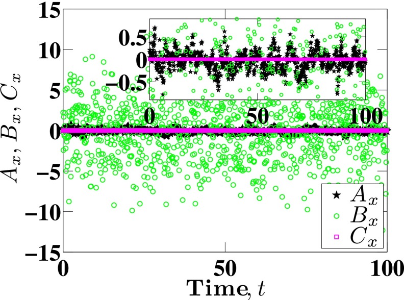
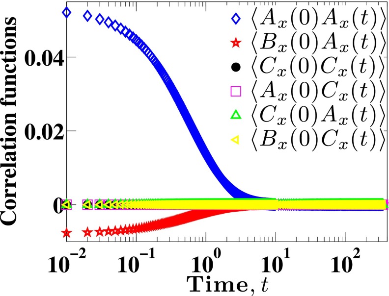
In order to compute DL through Eq. (11), we need to compute the correlations between the quantities Ax, Bx and Cx appearing in Eq. (14). These quantities are readily obtained during the integration of Eq. (7). Before proceeding to examining the correlations themselves, it is illuminating to examine first the order of magnitude of the different terms and their fluctuations. As an illustrative example, Fig. 1 presents these data for 100 reduced time units from a single trajectory. The values of Ax, Bx and Cx fluctuate around zero, but the magnitude of their fluctuations varies widely. The fluctuations in Bx are the largest, followed by Ax and then Cx. The results in Fig. 1 suggest that all of the correlation functions involving Cx will be very small. Figure 2 shows that this is indeed the case, with the four correlation functions involving the term Cx being very small in comparison to those excluding the term Cx. This result can be understood in terms of the variance σ2 of the different quantities. For example, the particular subset of data in Fig. 1 leads to , and . As a result, we will assume that all contributions involving Cx make a negligible contribution to DL. In other words, we conclude that the drift created due to the monomer concentration gradient, although non-zero in confinement, plays little role in the long-time diffusivity. Note that this does not mean that we can neglect the term when integrating Eq. (7), since that would lead to unphysical drift of the center-of-mass during the dynamic simulation. To compute DL, we need to integrate correlation functions such as those appearing in Fig. 2. We use 64-point Gaussian quadrature to calculate these integrals numerically. Note that the total data set for a given correlation function typically contain around 105 points, so this quadrature is still very small and allows us to capture the details of the tail of the correlation function. To test for the convergence of integrals in Eq. (12), we calculate the cumulative integrals,
| (15) |
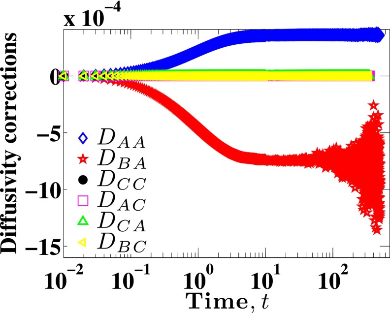
for different upper bounds, t. The resulting cumulative integrals for all correction terms are shown in Fig. 3. In an ideal case,
| (16) |
However, the data in the tails of the correlation become noisier as time-lag increases because the number of sample points decreases. Nevertheless, reaches a stable value for some large t before the sampling error becomes substantial. As expected from the correlation data shown in Fig. 2, the correction terms DCC, DAC, DCA, and DBC are negligible compared to DAA and DBA. We thus conclude that Eq. (11) can be written as
| (17) |
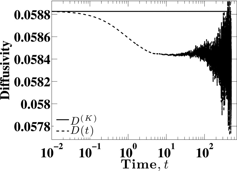
The only quantity that remains to be calculated is the Kirkwood diffusivity. The Kirkwood diffusivity is calculated using one-dimensional form of Eq. (1) or Eq. (S-7) of the supplementary material,44 where is generated for the configuration in each time step using Eq. (6). For this case study, we found that D(K) = 0.05883 ± 0.00002. Figure 4 shows how the diffusivity depends on time. It is clear that , and the overall shape of the curve is reminiscent of results obtained in free solution.24
FIG. 1.
Relative magnitudes of Ax, Bx, and Cx as functions of time for Nb = 11 and H = 10. The figure in the inset is the zoomed-in view to show that the magnitude of Cx is much smaller than that of Ax.
FIG. 2.
Mean correlation functions of an 11 bead chain as functions of time in a channel of size H = 10.
FIG. 3.
Six different diffusivity correction terms DAA, DBA, DCC, DAC, DCA, DBC for Nb = 11 and for H = 10 as functions of time.
FIG. 4.
Illustration of the drop in the diffusivity from its Kirkwood value to DL for Nb = 11 and H = 10.
B. Diffusivity corrections: Error analysis
Due to the finite number of data points available for long times, there is always sampling error in the tails of the correlation data in Fig. 2. As a result, we cannot estimate DΘΦ by simply using , where is the maximum value of the simulation time. In order to arrive at a reasonable estimate for DΘΦ and its uncertainty, we average over a subset of the data
| (18) |
where is the number of data points between some lower bound tl and upper bound tu and Δtc = 0.01 is the interval used for computing correlation functions. The corresponding error in DΘΦ is estimated by the method of Chodera et al.46 from the time series of data in this interval. For a given data set, the lower bound tl is decided visually by eye such that tl is always greater than the time at which the values of diffusivity corrections level off. We use tu = 500 as the upper bound for any data set for which there are at least 30 000 data points between tl and tu. Note that the time series of these 30 000 data points is not completely uncorrelated. Therefore, the effective number of uncorrelated data points46 turns out to be of the order of 100 in our study, which is the source of the error bar on DΘΦ. The value of tu = 500 excludes the poor sampling for long times (e.g., consider DBA in Fig. 3) because the total simulation length is typically 3 × 10⁵; a typical correlation function at t = 500 includes 108 data points. In some cases, when the convergence of diffusivity corrections was not achieved until tl = 500, the upper bound was chosen up to be tu = 3000. For instance, for the largest channel H = 50, we used tu = 2500 for Nb = 21 and tu = 3000 for Nb = 41. For the longest chains and largest channel sizes, the region between tl and tu becomes relatively small, leading to the largest errors in DΘΦ. The correlation and diffusivity correction data for these cases, along with many other cases covering the range of parameters used in this work, are shown in the supplemental material.44
C. Convergence of DL with respect to simulation time
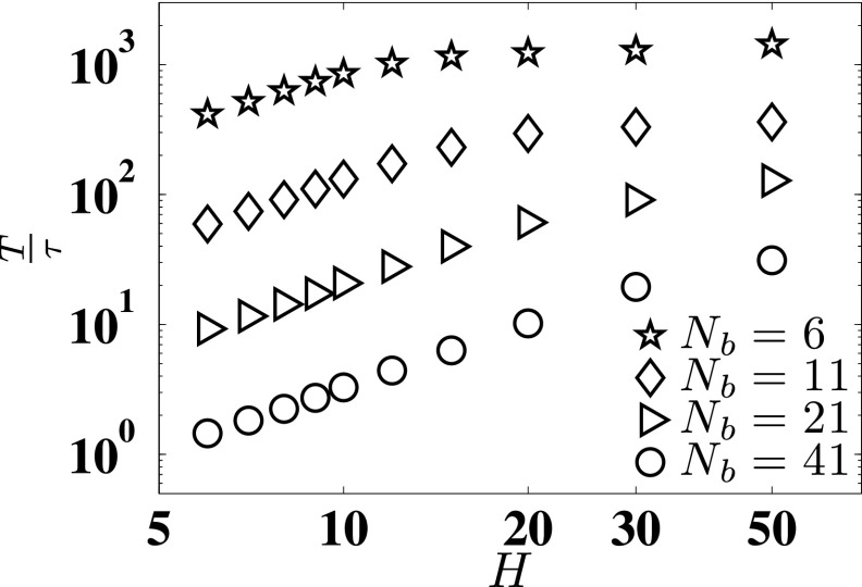
As we noted in the introduction, reaching the asymptotic limit for DL implied by Eq. (2) may require extremely long simulations. To quantify this statement, Fig. 5 shows the duration of our BD simulations, T, relative to the center-of-mass diffusion time for a particular molecular weight and channel size. In the latter, is the mean-square radius of gyration, which we use instead of the mean span of the confined DNA molecule to be consistent with prior work in free solution.24 Simulations in free solution24 suggest that a value T/τ ≈ 102 is required to obtain the asymptotic limit for DL. For the smaller chains and larger channels, our simulations appear to reach this heuristic for the simulation time. For longer chains and smaller channels, it is infeasible to run simulations for T/τ ≈ 102. For example, consider the worst case scenario Nb = 41 and H = 6. For this case, we obtain the diffusion time τ ≈ 2.41 × 10⁵. We used one week of CPU time to run the BD simulation for T = 3.25 × 10⁵, roughly the same as the diffusion time. To achieve T/τ ≈ 100 would require two years to obtain a single data point. While such a calculation may be of theoretical interest, it is not particularly interesting in practice—as we noted in the introduction, a simulation time of T = 3.25 × 10⁵ corresponds to around 10 min and thus exceeds a typical image acquisition time in experiments. Moreover, it is not entirely clear that the heuristic limit T/τ ≈ 102 to obtain DL in free solution24 will hold in confinement. First, the configurational phase space in confinement is considerably smaller than in free solution. Second, and more importantly, the solid walls provide hydrodynamic screening and thus remove correlations between different parts of chain. Both of these factors suggest that the asymptotic limit may be reached more quickly in confinement than in free solution even after taking into account the slowing of the dynamics by polymer-wall friction.
FIG. 5.
Length of BD simulation T relative to the center-of-mass diffusion time of the chain τ.
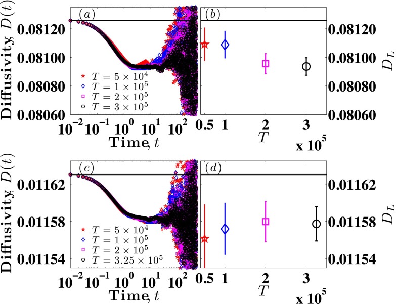
Since there is no a priori argument to suggest a good heuristic for T/τ in confinement, we investigated the convergence of the value of DL as a function of simulation time T for the smallest channel H = 6, which we presume will be the slowest to converge. Figures 6(a) and 6(c) plot the values of D(t) obtained using four different values of T for the shortest chain (Nb = 6) and the longest chain (Nb = 41), respectively. The data in these figures, which are analogous to Fig. 4, suggest that the diffusivity is independent of the upper bound T for sufficiently large T. To be more quantitative, Figs. 6(b) and 6(d) plot the values of DL obtained for both molecular weights, respectively, as a function of simulation time T. It is clear that the difference between mean values of DL for the two longest times is not statistically significant, having p-values of 0.834 for Nb = 6 and 0.935 for Nb = 41. Table I shows the p-values for all pairs of simulation lengths. Note that while calculating the p-values, the degree of freedom was 32 (effective number of uncorrelated data points) in these cases.
FIG. 6.
Convergence of DL for Nb = 6 and 41. (a) Time series D(t) based on different simulation lengths for Nb = 6, H = 6. (b) Mean value of DL as a function of simulation length T for Nb = 6, H = 6. (c) Time series D(t) based on different simulation lengths for Nb = 41, H = 6. (d) Mean value of DL as a function of simulation length T for Nb = 41, H = 6. Solid black lines in all four subplots indicate corresponding values of D(K) for that molecular weight.
TABLE I.
p-values for various pairs of simulations lengths for both Nb = 6 (upper triangular matrix highlighted by italic cells) and Nb = 41 (lower triangular matrix highlighted by boldface cells). T⋆ denotes that it is different for both chains; for Nb = 6, x = 3 and for Nb = 41, x = 3.25.
| T = 5 × 10⁴ | T = 1 × 10⁵ | T = 2 × 10⁵ | T⋆ = x × 105 | |
|---|---|---|---|---|
| T = 5 × 10⁴ | 1 | 0.9862 | 0.3163 | 0.2356 |
| T = 1 × 10⁵ | 0.8204 | 1 | 0.2581 | 0.1748 |
| T = 2 × 10⁵ | 0.6691 | 0.8243 | 1 | 0.8340 |
| T⋆ = x × 105 | 0.6988 | 0.8693 | 0.9345 | 1 |
D. Effect of molecular weight and channel size
We repeated the analysis described in Sec. IV A for Nb = 11 and H = 10 for the other 39 combinations of molecular weight and channel size. We find the same trend for all sets of parameters, namely, that there are only two dominating diffusivity correction terms DAA and DBA, and the others are negligible. Plots of correlation functions and diffusivity corrections for some of the parameters sets are shown in the supplementary material44 to show the generality of this trend. We also include a table of Kirkwood diffusivity values for each combination of Nb and H in the supplementary material.44 These data allow one to produce the equivalent of Fig. 4 for different channel sizes and molecular weights through Eq. (17).
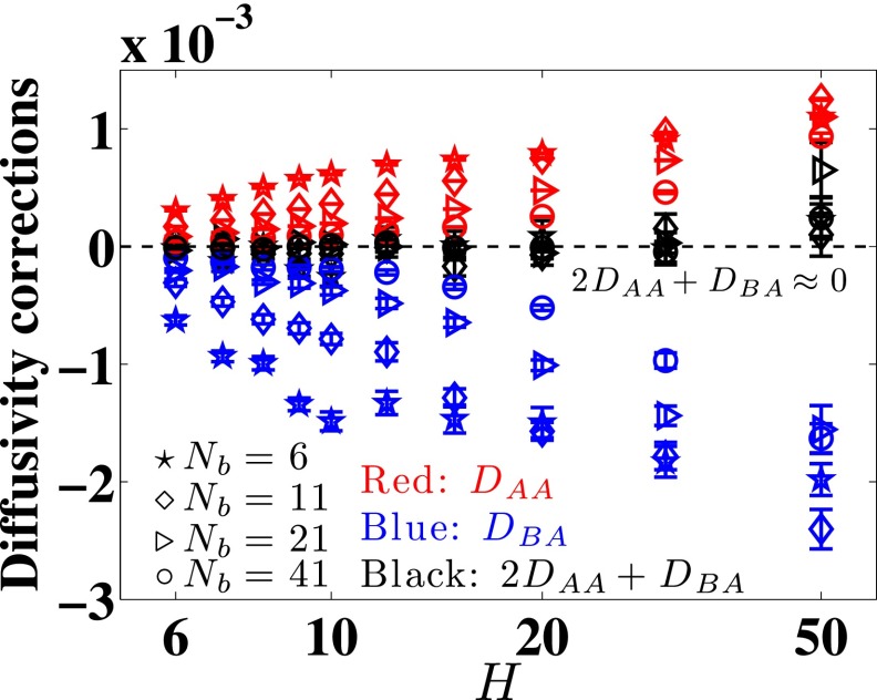
A careful inspection of Fig. 3 suggests that DBA ≈ −2DAA, which is also the case from Brownian dynamics simulations in free solution.24 Figure 7 shows that this is indeed the case for all channel sizes and molecular weights, except for channel size H = 50. The data for H = 50, which correspond to weak confinement for all of the chain sizes considered here, have relatively larger error bars for all chains. We cannot confirm DBA ≈ −2DAA for this channel. However, for all other parameters, we can infer that
| (19) |
We emphasize that this is not proof of the equality DBA = −2DAA, but rather data suggesting that such an equality likely holds in confinement.
FIG. 7.
Converged values of DAA and DBA for a range of channels sizes and chain sizes. The black data points, except for H = 50, show that DBA ≈ − 2DAA.
The corrections to the diffusion coefficient in channel confinement are essentially the same as those found by Liu and Dünweg24 in Brownian dynamics simulations of a polymer chain in free solution. Note, however, a subtle difference in methodology; the Kirkwood diffusivity in free solution is calculated using Eq. (1), not the one-dimensional form of Eq. (1) or Eq. (S-7) of the supplementary material,44 and the correction terms are calculated using the 3D version of Eqs. (11)–(13), where DAA and DBA are given by
| (20) |
with A and B being the vectors defined in Eq. (14).
As a result of Eq. (19), Eq. (17) can further be simplified to
| (21) |
which is exactly the same relationship derived by Fixman18 for free solution for long-time diffusivity in the theoretical limit. Moreover, since DAA is positive in confinement, we further find that
| (22) |
again in agreement with Fixman's results for free solution for long-time diffusivity in the theoretical limit.18
We are now at the stage where we can achieve our original goal of assessing the accuracy of the Kirkwood approximation in channel-confinement. Following the standard convention in the literature,18,20 we define the quantity
| (23) |
as the percent error due to Kirkwood approximation. Using Eq. (17), we can also express this deviation in terms of the significant correction terms,
| (24) |
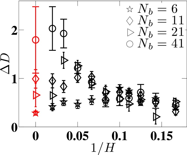
Figure 8 presents the error ΔD in the Kirkwood approximation for all of the simulations included in our analysis. The error is always less than about 2%.
FIG. 8.
ΔD for a range of channel sizes and chain sizes. Note that the red data for 1/H = 0 correspond to free solution data.
V. DISCUSSION
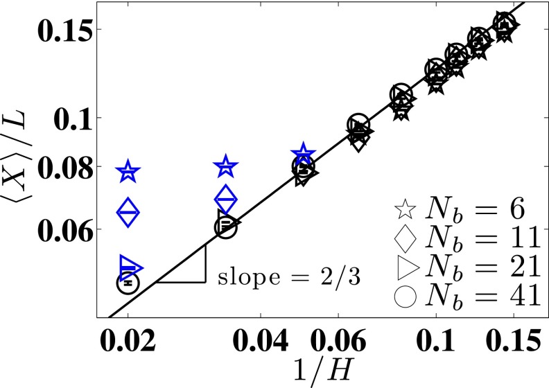
Many of the results for channel-confined DNA mimic those in free solution, most notably Eqs. (19) and (22) and the negligible contribution to DL from Cx (which is identically zero in free solution). We also observe an increase in the error for the Kirkwood approximation in free solution as the molecular weight increases. Similar to Liu and Dünweg,24 we cannot reach sufficiently high molecular weights to determine whether the error in the Kirkwood diffusivity for this DNA model continues to increase as Nb increases further or whether it plateaus at some point. Overall, the relatively low error of the Kirkwood approximation for DNA in free solution is encouraging because we have used the Kirkwood approximation elsewhere47 to make broader conclusions about the utility of DNA as a model polymer. An important feature of the key result in Fig. 8 is the collapse of the data for the smaller channel sizes. To understand the collapse, we note that the data in this figure correspond to three cases: (i) free solution (H → ∞), (ii) weak confinement (H ≳ Rg), and (iii) the de Gennes regime. To distinguish more quantitative between cases (ii) and (iii), Fig. 9 plots the mean span,
| (25) |
of the chain as a function of the inverse channel size. In the latter, Ri,x is the x component of the position vector Ri of bead i. Those data lying on the de Gennes scaling law,28
| (26) |
correspond to confinement in the de Gennes regime. The remaining data represent weak confinement; the DNA experiences hydrodynamic (and excluded volume) interactions with the walls, but it has not yet achieved the blob-like configuration that characterizes confinement in the de Gennes regime because the molecular weight is too low.
FIG. 9.
The ratio of mean extension to contour length L of the chain as a function of channel size H for four different chain sizes. The solid line is Eq. (26) for the de Gennes scaling for the extension of a chain in a nanochannel. The blue symbols are weak confinement, and the black symbols are those chains that are long enough to be in the de Gennes regime.
Once the chains are long enough to be in the de Gennes regime, we can understand the error in the Kirkwood approximation (as well as the collapse of the data in Fig. 8) through the blob hydrodynamics ideas of Brochard and de Gennes.9 In blob theory, each subchain of size
| (27) |
is envisioned as a swollen excluded volume subchain of length Lblob that is hydrodynamically decoupled from the other blobs through the screening provided by the walls. As a result, the properties of the chain are readily computed by determining the properties of a single blob and then summing up the contribution due to the
| (28) |
blobs in the chain. For example, blob theory leads to the scaling in Eq. (26) for the chain extension by noting that span of the confined chain is .
In blob theory, the diffusivity of the chain with hydrodynamically independent blobs is given by9
| (29) |
where ζblob is the friction coefficient of a blob and Dblob is the corresponding diffusivity of a blob. Naturally, we would expect that the friction coefficient of a blob in the short-time limit will differ from that in the longer time limit. If we denote these diffusivities as and Dblob,L, respectively, and insert Eq. (29) in the definition of ΔD in Eq. (23), we arrive at
| (30) |
The latter result is independent of the length of the chain, which explains the collapse of the data in Fig. 8. When we combine Eq. (30) with the dependence of ΔD on Nb in free solution in Fig. 8 and prior work,24 we can also rationalize the drop in ΔD with increasing confinement in the de Gennes regime. As we reduce H, Eq. (27) indicates that the length of the subchain comprising that blob is reduced as well. Since the error in the Kirkwood approximation decreases with decrease in molecular weight in free solution for any of the blob sizes here (since ΔD decreases for all of the chain sizes Nb that we studied and Nb > Nblob by definition), blob theory implies that the error in the Kirkwood approximation also decreases with the decrease in blob size.
The mean values of ΔD in Fig. 8 for chains that are not in the de Gennes regime suggest that there might be a maximum in ΔD as channel size increases and approaches infinity (free solution case). However, due to relatively large error bars on ΔD in the weak confinement regime, we cannot confirm such a peak using our simulation results. However, if there really exists such a maximum or if ΔD decreases as channel size increases beyond that required to have a single blob, it might be due to the reduction in the frequency of the monomer-wall hydrodynamic interactions, which is one of the source of the error due to Kirkwood approximation (other than monomer-monomer HI).
VI. CONCLUDING REMARKS
Using a Brownian dynamics simulation algorithm with excluded volume and hydrodynamic interactions (HI),10 we have shown that the error in the Kirkwood diffusivity decreases with the increase in confinement in the de Gennes regime due to the screening of hydrodynamic interactions between blobs. Overall, the error in the Kirkwood approximation is rather small for this DNA model, peaking at around 2% in weak confinement for a relatively large chain. Moreover, the error becomes independent of chain length once the polymer is large enough to be confined by the channel. These results lend support to conclusions about the diffusivity of DNA drawn from the Kirkwood approximation in both free solution47 and confinement.13,17
A key open question concerns how the error in the Kirkwood approximation changes as confinement increases further. In particular, we are motivated in our work by genome mapping in nanochannels,4 which takes place in channel sizes close to the 50 nm persistence length of DNA, an order of magnitude smaller than the smallest channel size considered here. As the channel size approaches the persistence length, the de Gennes blob theory breaks down and it is not obvious whether hydrodynamic conclusions drawn from a blob model apply to even stronger confinement. However, we have reason to be optimistic that the error in stronger confinement will be no worse (and probably better) than in the de Gennes regime. The error in the Kirkwood approximation arises from correlations in the monomer-monomer and monomer-wall hydrodynamic interactions. As we increase the confinement further, there is a decrease in both (i) the number of monomers inside the hydrodynamic screening volume H3 and (ii) the range of possible distances between a monomer and the wall. As a result, we would expect that the correlations in monomer-monomer HI and monomer-wall HI will both decrease; in the former case, due to a reduction in the number of monomer-monomer pairs, in the latter case, due to a reduction in the magnitude of the fluctuations in monomer-wall HI.
Testing this hypothesis about the accuracy of the Kirkwood approximation in strong confinement is not a simple task. The coarse-grained DNA model that we used here, which has a discretization of almost 40 persistence lengths per spring, is only valid in the de Gennes regime. This model breaks down in stronger confinement because it is unable to resolve the chain configurations at the length scale of a persistence length. There are other options to model polymers in such strong confinement, such as the touching-bead model48 that we have used previously in our studies of the Kirkwood diffusivity of DNA in confinement.13 Unfortunately, dynamic simulations of the touching-bead model would likely require simulating thousands of beads to reach the long-chain limit. Moreover, it seems likely that the relaxation time scales quadratically with molecular weight, making such simulations extremely expensive.
Ultimately, we suspect that detailed simulation of the dynamics of DNA confined in very small channels is not necessary to model the practical circumstances of interest such as genome mapping. Our results indicate that the Kirkwood approximation is quite accurate for DNA in the accessible regimes of confinement for a simulation. Moreover, it seems unlikely that there would be a sharp increase in the error of the Kirkwood approximation when confinement is increased further. Given the inherent uncertainty in any experiment relative to the error in the Kirkwood approximation, we conclude that the Kirkwood approximation is a useful tradeoff between simulation cost and time for modeling the diffusivity of confined DNA.
ACKNOWLEDGMENTS
This work was supported by the National Institutes of Health (R01-HG006851). Computational resources were provided in part by the University of Minnesota Supercomputing Institute.
References
- 1.Berndsen Z. T., Keller N., Grimes S., Jardine P. J., and Smith D. E., Proc. Natl. Acad. Sci. USA 111, 8345 (2014). 10.1073/pnas.1405109111 [DOI] [PMC free article] [PubMed] [Google Scholar]
- 2.Dorfman K. D., Rev. Mod. Phys. 82, 2903 (2010). 10.1103/RevModPhys.82.2903 [DOI] [Google Scholar]
- 3.Tegenfeldt J., Prinz C., Cao H., Chou S., Reisner W., Riehn R., Wang Y. M., Cox E. C., Sturm J. C., Silberzan P., and Austin R. H., Proc. Natl. Acad. Sci. USA 101, 10979 (2004). 10.1073/pnas.0403849101 [DOI] [PMC free article] [PubMed] [Google Scholar]
- 4.Lam E. T., Hastie A., Lin C., Ehrlich D., Das S. K., Austin M. D., Deshpande P., Cao H., Nagarajan N., Xiao M., and Kwok P.-Y., Nat. Biotechnol. 30, 771 (2012). 10.1038/nbt.2303 [DOI] [PMC free article] [PubMed] [Google Scholar]
- 5.Bird R. B., Curtiss C. F., Armstrong R. C., and Hassager O., Dynamics of Polymeric Liquids, Kinetic Theory Vol. 2 ( John Wiley & Sons, New York, 1986). [Google Scholar]
- 6.Karpusenko A., Carpenter J. H., Zhou C., Lim S. F., and Riehn R., J. Appl. Phys. 111, 024701 (2012). 10.1063/1.3675207 [DOI] [PMC free article] [PubMed] [Google Scholar]
- 7.Tree D. R., Wang Y., and Dorfman K. D., Biomicrofluidics 7, 054118 (2013). 10.1063/1.4826156 [DOI] [PMC free article] [PubMed] [Google Scholar]
- 8.Graham M. D., Annu. Rev. Fluid Mech. 43, 273 (2011). 10.1146/annurev-fluid-121108-145523 [DOI] [Google Scholar]
- 9.Brochard F. and de Gennes P. G., J. Chem. Phys. 67, 52 (1977). 10.1063/1.434540 [DOI] [Google Scholar]
- 10.Jendrejack R. M., Schwartz D. C., Graham M. D., and de Pablo J. J., J. Chem. Phys. 119, 1165 (2003). 10.1063/1.1575200 [DOI] [Google Scholar]
- 11.Chen Y.-L., Biomicrofluidics 7, 054119 (2013). 10.1063/1.4826157 [DOI] [PMC free article] [PubMed] [Google Scholar]
- 12.Chen Y.-L., Lin Y., Chang J.-F., and Lin P.-K., Macromolecules 47, 1199 (2014). 10.1021/ma401923t [DOI] [Google Scholar]
- 13.Tree D. R., Wang Y., and Dorfman K. D., Phys. Rev. Lett. 108, 228105 (2012). 10.1103/PhysRevLett.108.228105 [DOI] [PMC free article] [PubMed] [Google Scholar]
- 14.Kirkwood J. G. and Riseman J., J. Chem. Phys. 16, 565 (1948). 10.1063/1.1746947 [DOI] [Google Scholar]
- 15.Kirkwood J. G., J. Polym. Sci. 12, 1 (1954). 10.1002/pol.1954.120120102 [DOI] [Google Scholar]
- 16.Tree D. R., Wang Y., and Dorfman K. D., Phys. Rev. Lett. 110, 208103 (2013). 10.1103/PhysRevLett.110.208103 [DOI] [PMC free article] [PubMed] [Google Scholar]
- 17.Dai L., Tree D. R., van der Maarel J. R. C., Dorfman K. D., and Doyle P. S., Phys. Rev. Lett. 110, 168105 (2013). 10.1103/PhysRevLett.110.168105 [DOI] [PMC free article] [PubMed] [Google Scholar]
- 18.Fixman M., Macromolecules 14, 1710 (1981). 10.1021/ma50007a019 [DOI] [Google Scholar]
- 19.Fixman M., J. Chem. Phys. 78, 1594 (1983). 10.1063/1.444850 [DOI] [Google Scholar]
- 20.Fixman M., J. Chem. Phys. 84, 4080 (1986). 10.1063/1.450070 [DOI] [Google Scholar]
- 21.Zimm B. H., Macromolecules 13, 592 (1980). 10.1021/ma60075a022 [DOI] [Google Scholar]
- 22.Garcia de la Torre J., Jimenez A., and Freire J. J., Macromolecules 15, 148 (1982). 10.1021/ma00229a030 [DOI] [Google Scholar]
- 23.Wang S. Q., Douglas J. F., and Freed K. F., J. Chem. Phys. 85, 3674 (1986). 10.1063/1.450937 [DOI] [Google Scholar]
- 24.Liu B. and Dünweg B., J. Chem. Phys. 118, 8061 (2003). 10.1063/1.1564047 [DOI] [Google Scholar]
- 25.Mansfield M. L., Douglas J. F., Irfan S., and Kang E.-H., Macromolecules 40, 2575 (2007). 10.1021/ma061069f [DOI] [Google Scholar]
- 26.Schmidt R., Cifre J., and Garcia de la Torre J., Eur. Phys. J. E 35, 130 (2012). 10.1140/epje/i2012-12130-x [DOI] [PubMed] [Google Scholar]
- 27.Reisner W., Morton K. J., Riehn R., Wang Y. M., Yu Z., Rosen M., Sturm J. C., Chou S. Y., Frey E., and Austin R. H., Phys. Rev. Lett. 94, 196101 (2005). 10.1103/PhysRevLett.94.196101 [DOI] [PubMed] [Google Scholar]
- 28.Daoud M. and de Gennes P. G., J. Phys. France 38, 85 (1977). 10.1051/jphys:0197700380108500 [DOI] [Google Scholar]
- 29.Odijk T., Phys. Rev. E 77, 060901(R) (2008). 10.1103/PhysRevE.77.060901 [DOI] [PubMed] [Google Scholar]
- 30.Wang Y., Tree D. R., and Dorfman K. D., Macromolecules 44, 6594 (2011). 10.1021/ma201277e [DOI] [PMC free article] [PubMed] [Google Scholar]
- 31.Chen Y.-L., Graham M. D., de Pablo J. J., Randall G. C., Gupta M., and Doyle P. S., Phys. Rev. E 70, 060901(R) (2004). 10.1103/PhysRevE.70.060901 [DOI] [PubMed] [Google Scholar]
- 32.Jendrejack R. M., de Pablo J. J., and Graham M. D., J. Chem. Phys. 116, 7752 (2002). 10.1063/1.1466831 [DOI] [Google Scholar]
- 33.Marko J. F. and Siggia E. D., Macromolecules 27, 981 (1994). 10.1021/ma00082a015 [DOI] [Google Scholar]
- 34.Marko J. F. and Siggia E. D., Macromolecules 28, 8759 (1995). 10.1021/ma00130a008 [DOI] [Google Scholar]
- 35.Jendrejack R. M., Schwartz D. C., de Pablo J. J., and Graham M. D., J. Chem. Phys. 120, 2513 (2004). 10.1063/1.1637331 [DOI] [PubMed] [Google Scholar]
- 36.Dorfman K. D., Gupta D., Jain A., Muralidhar A., and Tree D. R., Eur. Phys. J. Spec. Top. 223, 3179 (2014). 10.1140/epjst/e2014-02326-4 [DOI] [PMC free article] [PubMed] [Google Scholar]
- 37.Ermak D. L. and McCammon J. A., J. Chem. Phys. 69, 1352 (1978). 10.1063/1.436761 [DOI] [Google Scholar]
- 38.Ottinger H. C., Stochastic Processes in Polymeric Fluids ( Springer, Berlin, 1996). [Google Scholar]
- 39.In Eq. (7), we adopt the notation for the multiplicative noise, rather than the standard notation , to avoid possible confusion with the symbol Bx used in the derivation of the long-time diffusion coefficient in Sec. III.
- 40.Fixman M., J. Chem. Phys. 69, 1527 (1978). 10.1063/1.436725 [DOI] [Google Scholar]
- 41.Fixman M., Macromolecules 19, 1204 (1986). 10.1021/ma00158a043 [DOI] [Google Scholar]
- 42.Grassia P. S., Hinch E. J., and Nitsche L. C., J. Fluid Mech. 282, 373 (1995). 10.1017/S0022112095000176 [DOI] [Google Scholar]
- 43.Ando T., Chow E., Saad Y., and Skolnick J., J. Chem. Phys. 137, 064106 (2012). 10.1063/1.4742347 [DOI] [PMC free article] [PubMed] [Google Scholar]
- 44.See supplementary material at http://dx.doi.org/10.1063/1.4917269E-BIOMGB-9-012502 for: (i) the derivation of the axial long-time diffusivity, (ii) autocorrelation and diffusivity corrections for Nb = 6, 11, 21, and 41 in channel sizes H = 6, 8, 15, and 50, and (iii) Kirkwood diffusivities for all channel sizes and molecular weights.
- 45.In the literature on diffusion of polymers in free solution,18,24 the quantities DAA and DBA have been denoted by D1 and D2, respectively. Since there are so many combinations of subscripts in confinement, we adopted the notation of Eq. (11) to make the subsequent text easier to follow.
- 46.Chodera J. D., Swope W. C., Pitera J. W., Seok C., and Dill K. A., J. Chem. Theory Comput. 3, 26 (2007). 10.1021/ct0502864 [DOI] [PubMed] [Google Scholar]
- 47.Tree D. R., Muralidhar A., Doyle P. S., and Dorfman K. D., Macromolecules 46, 8369 (2013). 10.1021/ma401507f [DOI] [PMC free article] [PubMed] [Google Scholar]
- 48.Wang J. and Gao H., J. Chem. Phys. 123, 084906 (2005). 10.1063/1.2008233 [DOI] [PubMed] [Google Scholar]
Associated Data
This section collects any data citations, data availability statements, or supplementary materials included in this article.
Data Citations
- See supplementary material at http://dx.doi.org/10.1063/1.4917269E-BIOMGB-9-012502 for: (i) the derivation of the axial long-time diffusivity, (ii) autocorrelation and diffusivity corrections for Nb = 6, 11, 21, and 41 in channel sizes H = 6, 8, 15, and 50, and (iii) Kirkwood diffusivities for all channel sizes and molecular weights.


