

Abstract
Motivation: Expression quantitative trait loci (eQTL) studies have discovered thousands of genetic variants that regulate gene expression, enabling a better understanding of the functional role of non-coding sequences. However, eQTL studies are costly, requiring large sample sizes and genome-wide genotyping of each sample. In contrast, analysis of allele-specific expression (ASE) is becoming a popular approach to detect the effect of genetic variation on gene expression, even within a single individual. This is typically achieved by counting the number of RNA-seq reads matching each allele at heterozygous sites and testing the null hypothesis of a 1:1 allelic ratio. In principle, when genotype information is not readily available, it could be inferred from the RNA-seq reads directly. However, there are currently no existing methods that jointly infer genotypes and conduct ASE inference, while considering uncertainty in the genotype calls.
Results: We present QuASAR, quantitative allele-specific analysis of reads, a novel statistical learning method for jointly detecting heterozygous genotypes and inferring ASE. The proposed ASE inference step takes into consideration the uncertainty in the genotype calls, while including parameters that model base-call errors in sequencing and allelic over-dispersion. We validated our method with experimental data for which high-quality genotypes are available. Results for an additional dataset with multiple replicates at different sequencing depths demonstrate that QuASAR is a powerful tool for ASE analysis when genotypes are not available.
Availability and implementation: http://github.com/piquelab/QuASAR.
Contact: fluca@wayne.edu or rpique@wayne.edu
Supplementary information: Supplementary Material is available at Bioinformatics online.
1 Introduction
Quantitative trait loci (QTLs) for molecular cellular phenotypes (as defined by Dermitzakis, 2012), such as gene expression [expression QTL (eQTL)] (e.g. Stranger et al., 2007), transcription factor binding (Kasowski et al., 2010) and DNase I sensitivity (Degner et al., 2012) have begun to provide a better understanding of how genetic variants in regulatory sequences can affect gene expression levels (see also Gibbs et al., 2010; Gieger et al., 2008; Melzer et al., 2008; Stranger et al., 2007). eQTL studies in particular have been successful at identifying genomic regions associated with gene expression in various tissues and conditions (e.g. Barreiro et al., 2012; Dimas et al., 2009; Ding et al., 2010; Fairfax et al., 2014; Grundberg et al., 2011; Lee et al., 2014; Maranville et al., 2011; Nica et al., 2011; Smirnov et al., 2009). Although previous studies have shown an enrichment for GWAS hits among regulatory variants in lymphoblastoid cell lines (LCLs) (Nica et al., 2010; Nicolae et al., 2010), a full understanding of the molecular mechanisms underlying GWAS hits requires functional characterization of each variant in the tissue and environmental conditions relevant for the trait under study (e.g. estrogen level for genetic risk to breast cancer, Cowper-Sal·lari et al., 2012).
The ongoing GTEx project will significantly increase the number of surveyed tissues for which eQTL data are available and will represent a useful resource to functionally annotate genetic variants. However, the number of cell types and environments explored are a small subset of the presumably larger number of regulatory variants that mediate specific GxE interactions. eQTL studies are expensive, requiring large sample sizes (n > 70), which may be difficult to achieve for tissues that are obtained by surgical procedures or are difficult to culture in vitro. Even if biospecimens are readily available at no cost, eQTL studies require large amounts of experimental work to measure genotypes and gene expression levels. As the measurement of gene expression using high-throughput sequencing (RNA-seq) is becoming more popular than microarrays, RNA-seq library preparation is also becoming less expensive ($46/sample), whereas costs of sequencing are also very rapidly decreasing (e.g. 16M reads per sample would cost $49 using a multiplexing strategy). Additionally, the sequence information provided by RNA-seq can be used to call genotypes (Duitama et al., 2012; Piskol et al., 2013; Shah et al., 2009), detect and quantify isoforms (Katz et al., 2010; Trapnell et al., 2010) and to measure allele-specific expression (ASE), if enough sequencing depth is available (Degner et al., 2009; Pastinen, 2010).
ASE approaches currently represent the most effective way to assay the effect of a cis-regulatory variant within a defined cellular environment, while controlling for any trans-acting modifiers of gene expression, such as the genotype at other loci (Cowper-Sal·lari et al., 2012; Hasin-Brumshtein et al., 2014; Kasowski et al., 2010; Kukurba et al., 2014; McDaniell et al., 2010; McVicker et al., 2013; Pastinen, 2010; Reddy et al., 2012; Skelly et al., 2011). As such, ASE studies have greater statistical power to detect genetic effects in cis than a traditional eQTL mapping approach when using a small sample size. Additionally, ASE may also be useful to detect epigenetic imprinting of gene expression if ASE is present but no eQTL is detected (Degner et al., 2009; Seoighe et al., 2006).
In the absence of ASE, the two alleles for a heterozygous genotype at a single-nucleotide polymorphism (SNP) in a gene transcript are represented in a 1:1 ratio of RNA-seq reads. To reject the null hypothesis and infer ASE, it is necessary to first identify heterozygous SNPs with high confidence and then conduct inference to detect a departure from a 50% allelic ratio. Although genotyping and ASE are usually considered two separate problems, miscalling a homozygous SNP as heterozygous is likely to induce an error in rejecting the ASE null hypothesis; thus, we argue that the two problems should addressed together.
Although it is possible to obtain genotype information from RNA-seq (Duitama et al., 2012; Piskol et al., 2013; Shah et al., 2009), to the best of our knowledge, all existing methods for detecting ASE consider the genotypes known and error probabilities associated with genotyping are not taken into account for the ASE step. Although overall genotyping quality can also be modeled within the ASE model (McVicker et al., 2013), there is currently no method that for each SNP can jointly genotype and detect allelic imbalances in high-throughput sequencing data. An approach that takes into account base-calling errors was previously proposed for detecting ASE in ESTs data (Seoighe et al., 2006), but for RNA-seq data, it is essential to also include overdispersion. Here, we propose a novel framework for quantitative allele-specific analysis of reads (QuASAR) that starts from a single or multiple RNA-seq experiments from the same individual and can directly identify heterozygous SNPs and assess ASE accurately by taking into account base-calling errors and overdispersion in the ASE ratio. QuASAR is evaluated with two different datasets that demonstrate genotyping accuracy and the importance of incorporating the genotype uncertainty when performing ASE inference.
2 Materials and methods
2.1 QuASAR approach
QuASAR starts with experimental high-throughput sequencing data. Here, we focus on RNA-seq, but the same or similar pipeline can be applied to DNase-seq, ChIP-seq, ATAC-seq or other types of functional genomics library preparations. Figure 1 illustrates the underlying problem: detecting SNPs covered by a number of transcripts with high allelic imbalance and for which homozygosity (in the presence of base-calling errors) can also be rejected.
Fig. 1.
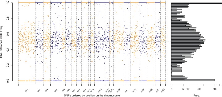
Reference allele frequency from reads overlapping SNPs. (Left) Each dot represents an SNP covered by at least 15 RNA-seq reads. The y-axis represents the fraction of RNA-seq reads that match the reference allele (observed ). The x-axis represents the order of the SNP position in a chromosome. (Right) Histogram showing the distribution of values across the genome. The three modes () correspond, respectively, to the three possible genotypes: homozygous reference (RR), heterozygous under no ASE (RA), and homozygous alternate (AA)
We focus our attention on sites that are known to be variable in human populations, specifically we consider all SNPs from the 1000 Genomes project (1KG) with a minor allele frequency (MAF) > 0.02. We index each SNP with and each sample by . All samples are from the same individual and may represent different experimental conditions or replicates. We only consider SNPs represented in at least 15 reads across all the samples. At each site l, three genotypes are possible being homozygous reference (RR), heterozygous (RA) or homozygous alternate (AA), respectively. For each sample s and site l, represents the total number of reads and take the value 1 if read k matches the reference allele and 0 if it matches the alternate allele. We can then model the data as a mixture model
| (1) |
where represents the prior probability associated with each genotype. The probability of the observed reads, , depends on the genotype. For Gl = 0:
| (2) |
where we will only observe reads matching the alternate allele if those are base-calling errors, here modeled by the parameter ϵs. Conversely, for Gl = 2, we have the following:
| (3) |
If the genotype is heterozygous Gl = 1, we observe reads from the reference allele with probability ρl or the alternate allele with probability (), resulting in the following model:
| (4) |
Considering that and Asl = Nsl – Rsl are, respectively, the number of reads from sample s observed at site l matching the reference allele and the alternate allele, the previous equations can be simplified as follows:
| (5) |
| (6) |
| (7) |
where and makes explicit that homozygotes, gl = 2 (or gl = 0), are indistinguishable from (or ) when gl = 1. In QuASAR, we resolve this identifiably problem by assuming that those cases with extreme ASE across all replicates are more likely to be homozygous genotypes.
To fit the mixture model, we use an expectation maximization (EM) algorithm (see Section 2 for more details) in which we estimate sample-specific base-calling error rates (ρ is fixed to 0.5) and posterior probabilities for the genotypes. For the ASE inference step, we wish to test the null hypothesis . We additionally consider that ψ in (5–7) is a random variable sampled from an ∼Beta distribution with:
| (8) |
where the hyper parameter Ms controls for over-dispersion and results in a better calibrated test as shown in Section 3. Combining (7) and (8) results in a beta-binomial distribution (13), which we use to model the number of reads coming from the reference allele. Formalized as a likelihood ratio test (LRT), the inference step takes into account over-dispersion and genotype uncertainty:
| (9) |
where the set of parameters are maximum likelihood estimates under the null hypothesis (see Section 2). To calculate a P value, we use the property that is asymptotically distributed as .
2.2 Model fitting and parameter estimation
To use the EM procedure (McLachlan and Krishnan, 2007), we first convert (1) to a ‘complete’ likelihood, as if we knew the underlying genotypes :
| (10) |
where are binary indicator variables and Θ represents the set of all parameters of the model. In log likelihood form we have:
| (11) |
During the genotyping step, to maintain identifiability of the model, we fix for all loci. Although Ms could also be estimated within the EM procedure, we only consider overdispersion on the ASE step. These two choices lead to a much simpler EM procedure and a slightly conservative estimate of ϵs.
2.2.1 E step
From the complete likelihood function (11), we derive the expected values for the unknown genotype indicator variables given the observed data and the current estimates for the model parameters. These quantities are also of interest for genotyping because they represent the posterior probabilities of each genotype given the data, :
| (12) |
The prior genotype probabilities are obtained from the 1KG allele frequencies assuming Hardy–Weinberg equilibrium, but the user can change this.
2.2.2 M step
Using the expected values from the E step, the complete likelihood is now a function of ϵs that is easily maximized
After we run QuASAR to infer genotypes across samples from the same individual, for each site we have a posterior probability of each genotype , and a base-calling error estimated for each sample. From these posteriors, discrete genotypes are called by using the genotype with the highest posterior probability; the maximum a posteriori (MAP) estimate.
2.2.3 ASE inference
To detect ASE, we only consider sites with an heterozygous MAP higher than a given threshold (e.g. ). We then test the possibility that ρsl deviates from 0.5 while also taking into account overdispersion using a beta-binomial model [combining (7) and (8)]:
| (13) |
where Ms controls the effective number of samples supporting the prior belief that and is estimated using grid search:
| (14) |
We estimate using (13) with from (14) and a standard gradient method (L-BFGS-B) to maximize the log-likelihood function
| (15) |
Finally, all parameters are used to calculate the LRT statistic in (9) and its P value.
Additionally, we can provide an estimate of the standard error associated with the parameter using the second derivative of the log-likelihood function (15):
| (16) |
Alternatively, we can also recover a standard error from (9) (as is asymptotically distributed as ), by using the P value to back solve for the standard error:
| (17) |
where is the quantile function for a standard normal distribution and pls is the P value from (9). We use the first form (16) when and (17) otherwise, as each provides a better approximation at those ranges. Alternatively, if we do not need , we can use (15) to obtain a profile likelihood confidence interval for ρsl.
2.3 Experimental data
LCLs (GM18507 and GM18508) were purchased from Coriell Cell Repository and human umbilical vein endothelial cells (HUVECs) from Lonza. LCLs were cultured and starved according to Maranville et al. (2011). Cryopreserved HUVECs were thawed and cultured according to the manufacturer protocol (Lonza), with the exception that 48 h prior to collection, the medium was changed to a starvation medium, composed of phenol-red free EGM-2, without hydrocortisone and supplemented with 2% charcoal stripped-FBS. Cells were washed 2X using ice cold phosphate-buffered saline, lysed on the plate, using Lysis/Binding Buffer (Ambion) and frozen at −80°C. mRNA was isolated using the Ambion Dynabeads mRNA Direct kit (Life Technologies). We then prepared libraries for Illumina sequencing using a modified version of the NEBNext Ultra Directional RNA-seq Library preparation kit (New England Biolabs). Briefly, each mRNA sample was fragmented (300 nt) and converted to double-stranded cDNA, onto which we ligated barcoded DNA adapters (NEXTflex-96 RNA-seq Barcodes, BIOO Scientific). Double-sided SPRI size selection (SPRISelect Beads, Beckman Coulter) was performed to select 350–500 bp fragments. The libraries were then amplified by polymerase chain reaction and pooled for sequencing on the Illumina HiSeq 2500 at the University of Chicago Genomics Core. For each LCL sample, libraries from nine replicates were pooled for a total of 42.3M and 34.9M 50-bp PE reads, respectively. We subsequently resequenced this libraries for a total of 81.0M and 78.6M 150-bp PE reads. For the HUVEC samples (267M reads total), we collected data for 18 replicates across six time points to capture a wide range of basal physiologic conditions.
2.4 Pre-processing
To create a core set of SNPs for ASE analysis, we first removed rare (MAF < 5%) variants from all 1KG SNPs (see Supplementary Material for an analysis without this step). We also removed SNPs within 25 bases upstream or downstream of another SNP or short InDels as well as SNPs in regions of annotated copy numbers or other blacklisted regions (Degner et al., 2012). Reads were aligned to the reference human genome hg19 using bwa mem (Li and Durbin, 2009, http://bio-bwa.sourceforge.net). Reads with quality <10 and duplicate reads were removed using samtools rmdup (http://github.com/samtools/). Using a mappability filter (Degner et al., 2012), we removed reads that do not map uniquely to the reference genome and to alternate genome sequences built considering all 1KG variants. Aligned reads were then piled up on the core set of SNPs using samtools mpileup command. Reads with an SNP at the beginning or at the end of the read, or with indels were also removed to avoid any potential experimental bias. Finally, the pileups were re-formatted, so that each SNP has a count for reads containing the reference allele and a count for those containing the alternate allele.
2.5 Comparison with other methods
To assess QuASAR genotyping quality, we focused on the LCL data and compared genotype calls to those of 1KG project. We also compared QuASAR genotyping accuracy to samtools + bcftools (Li and Durbin, 2009) and GATK (DePristo et al., 2011). To assess QuASAR ASE inference, we used QQ plots and eQTL derived from the GEUVADIS dataset (Lappalainen et al., 2013; Wen et al., 2014). When we compared QuASAR ASE inference to other methods, we used our implementation of the binomial and beta-binomial test by forcing QuASAR to ignore the genotyping uncertainty in the ASE inference step; i.e. in (9) numerator we only consider . For the binomial test, we further force . In the Supplementary Material, we also compared QuASAR performance to the method used in (Kukurba et al., 2014). To make the results comparable, we used QuASAR genotype information and the same pre-processing steps described above up to samtools mpileup.
3 Results
We implemented the QuASAR approach as detailed in Section 2 in an R package available at http://github.com/piquelab/QuASAR. First, to evaluate QuASAR genotyping accuracy, we collected RNA-seq data for two LCLs that already have high-quality genotype calls from the 1KG project (GM18507 and GM18508). As illustrated in Table 1 , we are able to accurately genotype thousands of loci with lower error rates than other methods commonly used for genotyping DNA-seq data. By design, QuASAR is more conservative in making heterozygous calls than homozygous calls, yet still retains a large number of heterozygous loci compared with GATK (DePristo et al., 2011) and samtools (Li and Durbin, 2009). In QuASAR, if there is contention between (i) an heterozygous genotype call with extreme allelic imbalance or (ii) an homozygous genotype call with base call errors, our model will favor the latter (ii). This is a crucial feature for accurate inference of ASE, which will be discussed later in more detail. As we increase the threshold on the QuASAR posterior probability of heterozygosity, we consistently reduce the genotype error rate, Supplementary Table S1.The error rates increase slightly if we include rare variants with MAF < 0.05 (Table S2) and are minimally affected when 1KG allele frequencies are not used as priors (Table S3). An important feature of QuASAR is that the genotyping information is also used for the next inference step.
Table 1.
QuASAR accuracy in genotyping heterozygous loci compared with GATK and samtools. Four samples with different sequencing depths and read lengths are compared. Each row reports the number of heterozygous SNPs identified by each method and the percentage of false discoveries when compared with 1KG genotypes. For GATK and samtools, we used the default parameter settings, and for QuASAR, we considered SNPs with a posterior probability of heterozygosity > 0.99
| Sample (no. of reads, read length) | Genotyping method |
|||
|---|---|---|---|---|
| Samtools | GATK | QuASAR | ||
| NA18507 (, 50 bp) | Number of hets | 3158 | 4568 | 3310 |
| FDR | 1.20% | 1.31% | 0.91% | |
| NA18508 (, 50 bp) | Number of hets | 2718 | 3933 | 2844 |
| FDR | 0.63% | 0.97% | 0.56% | |
| NA18507 (, 150 bp) | Number of hets | 19 515 | 24 522 | 17 434 |
| FDR | 1.29% | 2.09% | 1.14% | |
| NA18508 (, 150 bp) | Number of hets | 16 998 | 21 587 | 15 526 |
| FDR | 1.08% | 1.75% | 1.08% | |
We next sought to characterize QuASAR performance in genotyping and ASE inference from RNA-seq experiments sequenced at different depths. In total, we analyzed 18 samples (three replicates across six different time points) for an individual for which genotypes were not previously available. We combined the 18 fastq files in different ways as input for QuASAR to obtain an empirical power curve (Fig. 2). As expected, we observed that our ability to detect heterozygotes (MAP > 0.99) increases with the sequencing depth. At a more modest sequencing depth of 16 million, we can still detect more than 1,000 heterozygous sites.
Fig. 2.
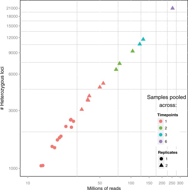
Empirical power in detecting heterozygous SNPs as a function of sequencing depth. Each point represents a single input dataset to QuASAR: either as a single experiment replicate and time point (red dot), combining multiple time points (2 = green, 3 = blue, 6 = purple) or combining replicates (1 = dot, 2 = triangle). The x-axis represents the total number of RNA-seq reads in the fastq input files. The y-axis represents the of the total number of SNPs that are determined to be heterozygous
After obtaining the genotypes, we assessed whether there is evidence of ASE at any of the SNPs determined to be heterozygous. To conduct ASE inference, we used the LRT (9) statistic in QuASAR and obtained P values. We controlled the FDR using the q-value procedure (Storey, 2002). As shown in Figure 3, our ability to detect ASE greatly increased with the number of SNPs we were able to genotype, which in turn is a function of coverage (Fig. 2). Using 100 million reads, we detected roughly 9,000 heterozygous SNPs of which 50 have ASE at 10%FDR.
Fig. 3.
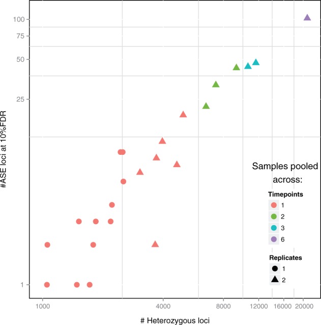
Empirical power in detecting ASE as a function of the number of heterozygous SNPs detected. Each point represents a single input dataset to QuASAR as in Figure 2. The x-axis represents the total number of SNPs that are determined to be heterozygous. The y-axis represents the of the number of SNPs that have a significant P value for ASE at 10% FDR
To assess the calibration of the ASE test in QuASAR and to compare it to other ASE inference approaches, we used QQ plots, Figure 4. A QQ plot compares the quantiles observed from a test statistic to those that are expected under a null distribution (e.g. P values are uniformly distributed between 0 and 1). The shape of the QQ-plot curve is useful to judge how well the P values are calibrated when we expect that a large number of the tests conducted are sampled from the null distribution. In this latter scenario, we expect that the QQ-plot curve would follow the 1:1 line for the range of P values with higher value. For small P values, we expect that the curve starts to depart from the 1:1 line representing the small proportion of tests that are not sampled from the null distribution. Many existing approaches for ASE use either a binomial test (Degner et al., 2012; Kukurba et al., 2014; McDaniell et al., 2010; Reddy et al., 2012) or a beta-binomial test (Pickrell et al., 2010; Sun, 2012) that does not account for genotyping or base-calling error. To compare QuASAR ASE inference to these alternative approaches, we used the RNA-seq data collected on the LCL samples and the genotype calls from QuASAR. Figure 4 clearly shows that the binomial test is too optimistic and will likely lead to many false discoveries. Another binomial test (Supplementary Fig. S1) independently implemented (Kukurba et al., 2014) show a similar behavior to our own implementation. In contrast to the binomial test, the beta-binomial model seems better calibrated but uncertainty on the genotype being a true heterozygote can lead to very small P values and false positives. QuASAR combines the beta-binomial model with uncertainty on the genotype, resulting in the most conservative approach, likely avoiding a common cause of false positives in ASE analysis.
Fig. 4.
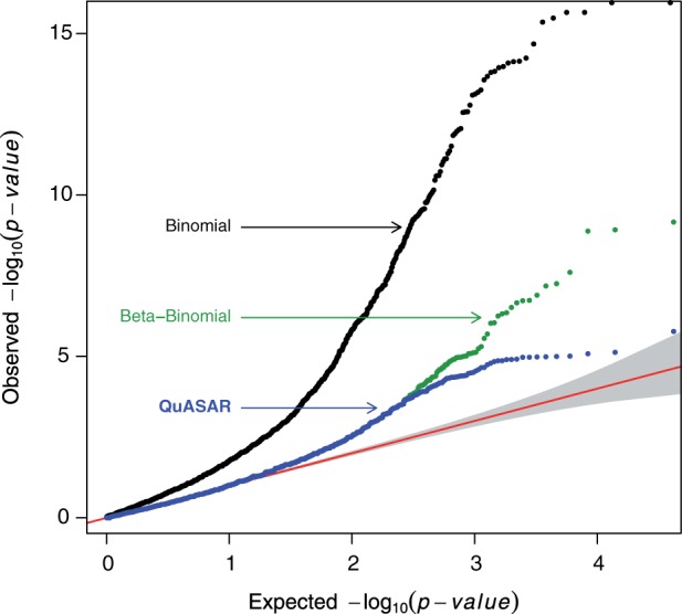
QQplot comparing the P value distribution of three alternative methods for determining ASE. The x-axis shows the quantiles of the P values expected from the null distribution. The y-axis shows the quantiles of the P values computed from the real data using three different methods: (i) binomial (black) assumes no overdispersion; (ii) beta-binomial (green) considers overdispersion but does not consider uncertainty in the genotype and (iii) QuASAR (blue) uses the beta-binomial distribution and uncertainty in the genotype calls. In all three cases, the same set of SNPs is considered. The shaded area in gray indicates a 95% confidence band for the null distribution
To further evaluate the differences between QuASAR and other methods, we focused on the high-coverage LCL samples. This cell type has been part of large sample eQTL studies such as GEUVADIS (Lappalainen et al., 2013) including RNA-seq data for more than 600 individuals. From a recent reanalysis of the GEUVADIS dataset (Wen et al., 2014), we selected genes with eQTLs (5% FDR) and a leading SNP with a high posterior inclusion probability (PIP > 0.9), as those are the nucleotides more likely to be causal (i.e. the eQTN). We hypothesized that in our data, genes for which the eQTN was heterozygote would be more likely to show evidence for ASE than those for which the eQTN was homozygote. However, transcripts with homozygous eQTNs could still show ASE, if they have additional personal/rare associations or due to an imprinting mechanism. In any of the methods we tested (Supplementary Fig. S2), there was a significant difference between ASE P values in the expected direction (Mann–Whitney U-test P < 0.02). The distribution of P values (Supplementary Fig. S2D) for ASE signals in transcripts with homozygous eQTNs are much closer to the uniform distribution in QuASAR when compared with other methods, especially those that do not account for overdispersion.
In general, the P values obtained across all methods tested are very much correlated to each other, as shown in Supplementary Figure S3, but there are key differences. The methods that use a binomial test tend to have lower P values than QuASAR, which uses a beta-binomial model. Supplementary Figure S4A and B show that we may observe more shrinkage for SNPs with deeper coverage. Compared with a test using the beta-binomial distribution but ignoring genotype uncertainty, our QuASAR test leads to similar P values, but SNPs with more uncertainty on being heterozygous are corrected in a higher degree toward a less significant P value (Supplementary Figs. S3C and S4C).
In terms of computational complexity, QuASAR is very fast. QuASAR runtime for genotyping with the EM procedure takes less than 20 s on any of our datasets (using a computer with a 6-core 2.93-GHz Intel processor and 8-GB RAM). Each EM iteration in the genotyping step is O(LS) linear with the number of SNPs and samples, and convergence is achieved in less than 20 iterations. GATK with the default options takes a longer amount of time (about 2 h) compared with samtools and QuASAR, as the latter methods focus directly on 1KG SNPs only. Comparatively, for both our pipeline and Kukurba et al. (2014), more time is spent in data pre-processing (roughly 10 min per sample depending on the sequencing depth and assuming reads are already aligned) than in genotyping or ASE inference.
4 Discussion
QuASAR is the first approach that detects genotypes and infers ASE from the same sequencing data. In this work, we focused on RNA-seq, but QuASAR can be applied to other data types (ChIP-seq, DNase-seq, ATAC-seq and others). Indeed, the more experimental data available from the same individual across many experimental samples (data types, conditions, cell types or technical replicates), the more certainty we can gather about the genotype.
A key aspect of the QuASAR ASE inference step is that it takes into account over-dispersion and genotype uncertainty resulting in a test that we have shown to be well calibrated. In many cases, the P values obtained from biased statistics can be recalibrated to the true null distribution using a permutation procedure. Unfortunately, this is not possible for ASE inference, as randomly permuting the reads assigned to each allele would inadvertently assume that the reads are distributed according to a binomial distribution. More complicated and computationally costly resampling procedures can be proposed, but it is not clear what additional assumptions may be introduced and if such methods can correctly take into account genotyping uncertainty.
If prior genotype information is available, it can also be provided as input to the algorithm. The prior uncertainty of the genotypes should be reflected in the form of prior probabilities for each genotype. In this article, we have shown that we can obtain reliable genotype information from RNA-seq reads, thus making additional genotyping unnecessary if the endpoint is to detect ASE. Instead, sequencing the RNA-seq libraries at a higher depth is probably a better strategy as it greatly improves the power to detect ASE.
Furthermore, as sequencing costs decrease rapidly, ASE methods are becoming very attractive in applications where eQTL studies have been previously used. This is of increased importance in scenarios where collecting a large number of samples is expensive or infeasible. Large-scale eQTL studies are still very much necessary for fine mapping, but analysis of ASE can provide unique insights into mechanisms that are uncovered only under specific experimental conditions, e.g. as a result of gene x environment interactions.
Supplementary Material
Acknowledgements
We thank Wayne State University HPC Grid for computational resources, the University of Chicago Genomics Core for sequencing services and Jacob Degner and members of the Luca/Pique group for helpful comments and discussions.
Funding
This work was supported by the National Institute of Health [1R01GM109215-01 to R.P.-R. and F.L.] and the American Heart Association [14SDG20450118 to F.L.].
Conflict of Interest: none declared.
References
- Barreiro L.B., et al. (2012) Deciphering the genetic architecture of variation in the immune response to Mycobacterium tuberculosis infection. Proc. Natl Acad. Sci. USA, 109, 1204–1209. [DOI] [PMC free article] [PubMed] [Google Scholar]
- Cowper-Sal lari R., et al. (2012) Breast cancer risk-associated SNPs modulate the affinity of chromatin for FOXA1 and alter gene expression. Nat. Genet., 44, 1191–1198. [DOI] [PMC free article] [PubMed] [Google Scholar]
- Degner J.F., et al. (2009) Effect of read-mapping biases on detecting allele-specific expression from RNA-sequencing data. Bioinformatics , 25,3207–3212. [DOI] [PMC free article] [PubMed] [Google Scholar]
- Degner J.F., et al. (2012) DNaseI sensitivity QTLs are a major determinant of human expression variation. Nature , 482, 390–394. [DOI] [PMC free article] [PubMed] [Google Scholar]
- DePristo M.A., et al. (2011) A framework for variation discovery and genotyping using next-generation DNA sequencing data. Nat. Genet., 43, 491–498. [DOI] [PMC free article] [PubMed] [Google Scholar]
- Dermitzakis E.T. (2012) Cellular genomics for complex traits. [DOI] [PubMed] [Google Scholar]
- Dimas A.S., et al. (2009) Common regulatory variation impacts gene expression in a cell type-dependent manner. Science , 325, 1246–1250. [DOI] [PMC free article] [PubMed] [Google Scholar]
- Ding J., et al. (2010) Gene expression in skin and lymphoblastoid cells: refined statistical method reveals extensive overlap in cis-eQTL signals. Am. J. Hum. Genet., 87, 779–789. [DOI] [PMC free article] [PubMed] [Google Scholar]
- Duitama J., et al. (2012) Towards accurate detection and genotyping of expressed variants from whole transcriptome sequencing data. BMC Genomics , 13(Suppl. 2), S6. [DOI] [PMC free article] [PubMed] [Google Scholar]
- Fairfax B.P., et al. (2014) Innate immune activity conditions the effect of regulatory variants upon monocyte gene expression. Science , 343, 1246949. [DOI] [PMC free article] [PubMed] [Google Scholar]
- Gibbs J.R., et al. (2010) Abundant quantitative trait loci exist for DNA methylation and gene expression in human brain. PLoS Genet., 6, e1000952. [DOI] [PMC free article] [PubMed] [Google Scholar]
- Gieger C., et al. (2008) Genetics meets metabolomics: a genome-wide association study of metabolite profiles in human serum. PLoS Genet., 4, e1000282. [DOI] [PMC free article] [PubMed] [Google Scholar]
- Grundberg E., et al. (2011) Global analysis of the impact of environmental perturbation on cis-regulation of gene expression. PLoS Genet., 7, e1001279. [DOI] [PMC free article] [PubMed] [Google Scholar]
- Hasin-Brumshtein Y., et al. (2014) Allele-specific expression and eQTL analysis in mouse adipose tissue. BMC Genomics , 15, 471. [DOI] [PMC free article] [PubMed] [Google Scholar]
- Kasowski M., et al. (2010) Variation in transcription factor binding among humans. Science , 328, 232–235. [DOI] [PMC free article] [PubMed] [Google Scholar]
- Katz Y., et al. (2010) Analysis and design of RNA sequencing experiments for identifying isoform regulation. Nat. Methods , 7, 1009–1015. [DOI] [PMC free article] [PubMed] [Google Scholar]
- Kukurba K.R., et al. (2014) Allelic expression of deleterious protein-coding variants across human tissues. PLoS Genet., 10, e1004304. [DOI] [PMC free article] [PubMed] [Google Scholar]
- Lappalainen T., et al. (2013) Transcriptome and genome sequencing uncovers functional variation in humans. Nature , 501, 506–511. [DOI] [PMC free article] [PubMed] [Google Scholar]
- Lee M.N., et al. (2014) Common genetic variants modulate pathogen-sensing responses in human dendritic cells. Science , 343, 1246980. [DOI] [PMC free article] [PubMed] [Google Scholar]
- Li H., Durbin R. (2009) Fast and accurate short read alignment with Burrows-Wheeler transform. Bioinformatics , 25, 1754–1760. [DOI] [PMC free article] [PubMed] [Google Scholar]
- Maranville J.C., et al. (2011) Interactions between glucocorticoid treatment and cis-regulatory polymorphisms contribute to cellular response phenotypes. PLoS Genet., 7, e1002162. [DOI] [PMC free article] [PubMed] [Google Scholar]
- McDaniell R., et al. (2010) Heritable individual-specific and allele-specific chromatin signatures in humans. Science , 328, 235–239. [DOI] [PMC free article] [PubMed] [Google Scholar]
- McLachlan G., Krishnan T. (2007) The EM Algorithm and Extensions , Vol. 382 John Wiley & Sons; New York, N.Y. [Google Scholar]
- McVicker G., et al. (2013) Identification of genetic variants that affect histone modifications in human cells. Science , 342, 747–749. [DOI] [PMC free article] [PubMed] [Google Scholar]
- Melzer D., et al. (2008) A genome-wide association study identifies protein quantitative trait loci (pQTLs). PLoS Genet., 4, e1000072. [DOI] [PMC free article] [PubMed] [Google Scholar]
- Nica A.C., et al. (2010) Candidate causal regulatory effects by integration of expression QTLs with complex trait genetic associations. PLoS Genet., 6, e1000895. [DOI] [PMC free article] [PubMed] [Google Scholar]
- Nica A.C., et al. (2011) The architecture of gene regulatory variation across multiple human tissues: the MuTHER study. PLoS Genet., 7, e1002003. [DOI] [PMC free article] [PubMed] [Google Scholar]
- Nicolae D.L., et al. (2010) Trait-associated SNPs are more likely to be eQTLs: annotation to enhance discovery from GWAS. PLoS Genet., 6, e1000888. [DOI] [PMC free article] [PubMed] [Google Scholar]
- Pastinen T. (2010) Genome-wide allele-specific analysis: insights into regulatory variation. Nat. Rev. Genet., 11, 533–538. [DOI] [PubMed] [Google Scholar]
- Pickrell J.K., et al. (2010) Understanding mechanisms underlying human gene expression variation with RNA sequencing. Nature , 464, 768–772. [DOI] [PMC free article] [PubMed] [Google Scholar]
- Piskol R., et al. (2013) Reliable identification of genomic variants from RNA-seq data. Am. J. Hum. Genet., 93, 641–651. [DOI] [PMC free article] [PubMed] [Google Scholar]
- Reddy T.E., et al. (2012) Effects of sequence variation on differential allelic transcription factor occupancy and gene expression. Genome Res., 22, 860–869. [DOI] [PMC free article] [PubMed] [Google Scholar]
- Seoighe C., et al. (2006) Maximum likelihood inference of imprinting and allele-specific expression from EST data. Bioinformatics , 22, 3032–3039. [DOI] [PubMed] [Google Scholar]
- Shah S.P., et al. (2009) Mutational evolution in a lobular breast tumour profiled at single nucleotide resolution. Nature , 461, 809–813. [DOI] [PubMed] [Google Scholar]
- Skelly D.A., et al. (2011) A powerful and flexible statistical framework for testing hypotheses of allele-specific gene expression from RNA-seq data. Genome Res., 21, 1728–1737. [DOI] [PMC free article] [PubMed] [Google Scholar]
- Smirnov D.A., et al. (2009) Genetic analysis of radiation-induced changes in human gene expression. Nature , 459, 587–591. [DOI] [PMC free article] [PubMed] [Google Scholar]
- Storey J.D. (2002) A direct approach to false discovery rates. J. R. Stat. Soc. Ser. B Stat. Methodol., 64, 479–498. [Google Scholar]
- Stranger B.E., et al. (2007) Population genomics of human gene expression. Nat. Genet., 39, 1217–1224. [DOI] [PMC free article] [PubMed] [Google Scholar]
- Sun W. (2012) A statistical framework for eQTL mapping using RNA-seq data. Biometrics , 68, 1–11. [DOI] [PMC free article] [PubMed] [Google Scholar]
- Trapnell C., et al. (2010) Transcript assembly and quantification by RNA-Seq reveals unannotated transcripts and isoform switching during cell differentiation. Nat. Biotechnol., 28, 511–515. [DOI] [PMC free article] [PubMed] [Google Scholar]
- Wen X., et al. (2014) Cross-population meta-analysis of eQTLs: fine mapping and functional study. bioRxiv. doi 10.1101/008797. [DOI] [PMC free article] [PubMed] [Google Scholar]
Associated Data
This section collects any data citations, data availability statements, or supplementary materials included in this article.