

Abstract
In this article, we propose a new method for principal component analysis (PCA), whose main objective is to capture natural “blocking” structures in the variables. Further, the method, beyond selecting different variables for different components, also encourages the loadings of highly correlated variables to have the same magnitude. These two features often help in interpreting the principal components. To achieve these goals, a fusion penalty is introduced and the resulting optimization problem solved by an alternating block optimization algorithm. The method is applied to a number of simulated and real datasets and it is shown that it achieves the stated objectives. The supplemental materials for this article are available online.
Keywords: Fusion penalty, Local quadratic approximation, Sparsity, Variable selection
1. Introduction
Principal component analysis (PCA) is a widely used data analytic technique that aims to reduce the dimensionality of the data for simplifying further analysis and visualization. It achieves its goal by constructing a sequence of orthogonal linear combinations of the original variables, called the principal components (PC), that have maximum variance. The technique is often used in exploratory mode and hence good interpretability of the resulting principal components is an important goal. However, it is often hard to achieve this in practice, since PCA tends to produce principal components that involve all the variables. Further, the orthogonality requirement often determines the signs of the variable loadings (coefficients) beyond the first few components, which makes meaningful interpretation challenging.
Various alternatives to ordinary PCA have been proposed in the literature to aid interpretation, including rotations of the components (Jollife 1995), restrictions for their loadings to take values in the set {—1,0,1} (Vines 2000), and construction of components based on a subset of the original variables (McCabe 1984). More recently, variants of PCA that attempt to select different variables for different components have been proposed and are based on a regularization framework that penalizes some norm of the PC vectors. Such variants include SCoTLASS (Jollife, Trendafilov, and Uddin 2003) that imposes an ℓ1 penalty on the ordinary PCA loadings and a recent sparse PCA technique (Zou, Hastie, and Tibshirani 2006) that extends the elastic net (Zou and Hastie 2005) procedure by relaxing the PC's orthogonality requirement.
In this article, we propose another version of PCA with sparse components motivated by the following empirical considerations. In many application areas, some variables are highly correlated and form natural “blocks.” For example, in the meat spectra example discussed in Section 4, the spectra exhibit high correlations within the high- and low-frequency regions, thus giving rise to such a block structure. Something analogous occurs in the image data, where the background forms one natural block, and the foreground one or more such blocks. In such cases, the loadings of the block tend to be of similar magnitude. The proposed technique is geared toward exploring such block structures and producing sparse principal components whose loadings are of the same sign and magnitude, thus significantly aiding interpretation of the results. We call this property fusion and introduce a penalty that forces “fusing” of loadings of highly correlated variables in addition to forcing small loadings to zero. We refer to this method as sparse fused PCA (SFPCA).
The remainder of the article is organized as follows. The technical development and computing algorithm for our method are presented in Section 2. An illustration of the method based on simulated data is given in Section 3. In Section 4, we apply the new method to several real datasets. Finally, some concluding remarks are drawn in Section 5.
2. The Model and Its Estimation
2.1 Preliminaries and Sparse Variants of PCA
Let X = (xi,j)n×p be a data matrix composed of n observations and p variables, whose columns are assumed to be centered. As noted above, PCA reduces the dimensionality of the data by constructing linear combinations of the original variables that have maximum variance; that is, for k = 1,…, p, define
| (2.1) |
where αk is a p-dimensional vector called factor loadings (PC vectors). The projection of the data Zk = Xαk is called the kth principal component. The technique proves most successful if one can use a small number k ≪ p of components to account for most of the variance and thus provide a relatively simple explanation of the underlying data structure. Some algebra shows that the factor loadings can be obtained by solving the following optimization problem:
| (2.2) |
where ∑^ = 1/n(XTX denotes the sample covariance of the data. The solution of (2.2) is given by the eigenvector corresponding to the kth largest eigenvalue of ∑^. An alternative way to derive the PC vectors, which proves useful in subsequent developments, is to solve the following constrained least squares problem:
| (2.3) |
where IK denotes a K × K identity matrix, ║M║F is the Frobenius norm of a matrix M , and A = [α1,…,αK] is a p × K matrix with orthogonal columns. The estimate  contains the first K PC vectors, and Ẑ = X the first K principal components.
To impose sparsity on the PC vectors, Jollife, Trendafilov, and Uddin (2003) proposed SCoTLASS, which adds an ℓ1-norm constraint to objective function (2.2), that is, for any 1 ≤ k ≤ K, solve
| (2.4) |
where is the ℓ1 norm of the vector α. Due to the singularity property of the ℓ1 norm, the constraint ║α║1 ≤ t shrinks some components of α to zero for small enough values of t. Therefore, objective function (2.2) produces sparse PC vectors. However, Zou, Hastie, and Tibshirani (2006) noted that in many cases, SCoTLASS fails to achieve sufficient sparsity, thus complicating the interpretation of the results. One possible explanation stems from the orthogonality constraint of the PC vectors that is not fully compatible with the desired sparsity condition. Hence, Zou, Hastie, and Tibshirani (2006) proposed an alternative way to estimate sparse PC vectors, by relaxing the orthogonality requirement. Their procedure amounts to solving the following regularized regression problem:
| (2.5) |
where βk is a p-dimensional column vector and B = [β1, β2,, …, βk]. The l2 penalty regularizes the loss function to avoid singular solutions, whenever n < p. If λ1 = 0, objective function (2.5) reduces to the ordinary PCA problem and the columns of B^ are proportional to the first K ordinary PC vectors (Zou, Hastie, and Tibshirani 2006); otherwise, the ℓ1 penalty ║βk║1 imposes sparsity on the elements of B^, that is, it shrinks some loadings exactly to zero. In addition, the first term in (2.5) can be written as
| (2.6) |
where A⊥ is any orthonormal matrix such that [A, A⊥] is a p × p orthonormal matrix. The quantity (αk − βk)T ∑^(αk− βk), 1 ≤ k ≤ p, measures the difference between αk and βk. Therefore, although there is no direct constraint on the column orthogonality in B, the loss function shrinks the difference between A and B and this results in the columns of B becoming closer to orthogonal. Numerical examples in the article by Zou, Hastie, and Tibshirani (2006) indicate that sparse PCA produces more zero loadings than SCoTLASS. However, both techniques cannot accommodate block structures in the variables, as the numerical results in Section 3 suggest. Next, we introduce a variant of sparse PCA called sparse fused PCA (SFPCA) that addresses this issue.
2.2 Sparse Fused Loadings
Our proposal is based on solving the following optimization problem:
| (2.7) |
where ; ρs,t denotes the sample correlation between variables Xs and Xt, and sign(•) is the sign function. The first penalty in (2.7) is the sum of l1 norms of the K PC vectors. It aims to shrink the elements of the PC vectors to zero, thus ensuring sparsity of the resulting solution. The second penalty is a linear combination of K generalized fusion penalties. This penalty shrinks the difference between βs,k and βt,k, if the correlation between variables Xs and Xt is positive; the higher the correlation, the heavier the penalty for the difference of coefficients. If the correlation is negative, the penalty encourages βs,k and βt,k to have similar magnitudes, but different signs. It is natural to encourage the loadings of highly correlated variables to be close, since two perfectly correlated variables with the same variance have equal loadings. First, highly correlated variables on the same scale pushing the loadings to the same value has the same effect as setting small regression coefficients to 0 in lasso: fitted model accuracy is not affected much, but interpretation is improved and overfitting avoided. Second, by definition of principal components, the kth PC vector maximizes the variance of subject to the orthogonality constraint. Since Xj's are centered, one can show that this variance equals to . Thus, in order to maximize the variance, we need the sign of βs,kβt,k to match the sign of cor(XS, Xt) (as far as the orthogonality constraint will allow). Finally, note that if two variables are highly correlated but have substantially different variances, their loadings will have different scales and will not be fused to the same value, which is the correct behavior for PCA on unscaled data. If this behavior is undesirable in a particular application, data should be standardized first (just like in regular PCA, it is the user's decision whether to standardize the data).
The effect of the fusion penalty, due to the singularity property of the ℓ1 norm, is that some terms in the sum are shrunken exactly to zero, resulting in some loadings having identical magnitudes. Therefore, the penalty aims at blocking the loadings into groups and “fusing” similar variables together for ease of interpretation. Finally, if ρs,t = 0 for any |t—s | > 1 and ρs,s+1 is a constant for all s, then the generalized fusion penalty reduces to the fusion penalty (Land and Friedman 1996; Tibshirani et al. 2005).
Note that one can use other types of weights in the generalized fusion penalty, including partial correlations or other similarity measures (Li and Li 2008).
2.3 Optimization of the Objective Function
We discuss next how to optimize the posited objective function. It is achieved through alternating optimization over A and B, analogously to the sparse PCA algorithm. Overall, the algorithm proceeds as follows.
Algorithm
Step 1. Initialize  by setting it to the ordinary PCA solution.
Step 2. Given A, minimizing the objective function (2.7) over B is equivalent to solving the following K separate problems:
| (2.8) |
where . The solution to (2.8) is nontrivial, and is discussed in Section 2.4. This step updates the estimate B^
Step 3. Given the value of B, minimizing (2.7) over A is equivalent to solving
| (2.9) |
The solution can be derived by a reduced rank Procrustes rotation (Zou, Hastie, and Tibshirani 2006). Specifically, we compute the singular value decomposition (SVD) of XTXB = UDVT and the solution to (2.9) is given by  = UVT. This step updates the estimate Â.
Step 4. Repeat Steps 2–3 until convergence.
2.4 Estimation of B Given A
Objective function (2.8) can be solved by quadratic programming. However, this approach can be inefficient in practice; thus, we propose a more efficient algorithm—local quadratic approximation (LQA) (Fan and Li 2001). This method has been employed in a number of variable selection procedures for regression and its convergence properties have been studied by Fan and Li (2001) and Hunter and Li (2005). The LQA method approximates the objective function locally via a quadratic form. Notice that
| (2.10) |
where and consequently sign .
After some algebra, one can show that (2.10) can be written as βTL(k)β, where L(k) = D(k) − W(k), W(k) = (ωS,t)p×p with diagonal elements equal to zero, and D(k)=diag(Σt≠1|ω1,t|,…,Σt≠p|ωp,t|).
Similarly, we have , where and . Then, (2.8) can be written as
| (2.11) |
Notice that (2.11) takes the form of a least squares problem involving two generalized ridge penalties; hence, its closed form solution is given by
| (2.12) |
Notice that both Ω(k) and L(k) depend on the unknown parameter βk. Specifically, LQA iteratively updates βk, L(k) and Ω(k) as follows, which constitute Step 2 of the Algorithm.
Step 2(a). Given β^k from the previous iteration, update Ω^(k) and L^(k).
Step 2(b). Given Ω^(k) and L^(k), update β^k by formula (2.12).
Step 2(c). Repeat Steps 2(a) and (b) until convergence.
Step 2(d). Scale β^k to have unit l2 norm.
Note that to calculate L(k) in Step 2(a), we need to calculate ωs,t = ρs,t/|βk,s—sign(ρs,t)βk,t|. When the values of βk,s and sign(ρs,t)βk,t are extremely close, ωs,t is numerically singular. In this case, we replace |βk,s−sign(ρs,t)βk,t | by a very small positive number (e.g., 10−10); similarly, we replace |βj,k| by a very small positive number if its value is extremely close to 0.
With the new Step 2, the Algorithm has two nested loops. However, the inner loop in Step 2 can be effectively approximated by a one-step update (Hunter and Li 2005), that is, by removing Step 2(c). In our numerical experiments, we found that this one-step update can lead to significant computational savings with minor sacrifices in terms of numerical accuracy.
2.5 Selection of Tuning Parameters
The proposed procedure involves two tuning parameters. One can always use cross-validation to select the optimal values, but it can be computationally expensive. We discuss next an alternative approach for tuning parameter selection based on the Bayesian information criterion (BIC), which we use in simulations in Section 3. In general, we found solutions from cross-validation and BIC to be comparable, but BIC solutions tend to be sparser.
Let and be the estimates of A and B in (2.7), obtained using tuning parameters λ1 and λ2. Let , where the columns of  contain the first K ordinary PC vectors of X. We define the BIC for sparse PCA as follows:
| (2.13) |
and analogously for SFPCA:
where dfSPCA and dfSFPCA denote the degrees of freedom of sparse and sparse-fused PCA defined as the number of all nonzero/nonzero-distinct elements in Bλ1,λ2, respectively. These definitions are similar to df defined for Lasso and fused Lasso (Tibshirani et al. 2005; Zou, Hastie, and Tibshirani 2007).
2.6 Computational Complexity and Convergence
Since XT X only depends on the data, it is calculated once and requires np2 operations. The estimation of A by solving an SVD takes O(pK2). Calculation of Ω and L in (2.11) requires O(p2) operations, while the inverse in (2.12) is of order O(p3). Therefore, each update in LQA is of order O(p3K), and the total computational cost is O(np2) + O(p3K).
The convergence of the algorithm essentially follows from standard results. Note that the loss function is strictly convex in both A and B, and the penalties are convex in B, and thus the objective function is strictly convex and has a unique global minimum. The integrations between Steps 2 and 3 of the Algorithm amount to block coordinate descent, which is guaranteed to converge for differentiable convex functions (see, e.g., Bazaraa, Sherali, and Shetty 1993). The original objective function has singularities, but the objective function (2.10) obtained from the local quadratic approximation that we are actually optimizing is differentiable everywhere, and thus the convergence of coordinate descent is guaranteed. Thus, we only need to make sure that each step of the coordinate descent is guaranteed to converge. In Step 3, we are optimizing the objective function (2.9) exactly and obtain the solution in closed form. In Step 2, the optimization is iterative, but convergence follows easily by adapting the arguments of Hunter and Li (2005) for local quadratic approximation obtained from general results for minorization-maximization algorithms.
3. Numerical Illustration of SFPCA
First, we illustrate the performance of the proposed SFPCA method on a number of synthetic datasets described next.
Simulation 1
This simulation scenario is adopted from the work of Zou, Hastie, and Tibshirani (2006). Three latent variables are generated as follows:
where V1, V2, and ε; are independent, and ε; ∼ N(0,1). Next, ten observable variables are constructed as follows:
where ε;j, 1 ≤ j ≤ 10, are iid N(0,1). The variances of the three latent variables are 290, 300, and 38, respectively. Notice that by construction, variables X1 through X4 form a block with a constant within-block pairwise correlation of 0.997 (“block 1”), while variables X5 through X8 and X9, X10 form another two blocks (“block 2” and “block 3,” respectively). Ideally, a sparse first PC should pick up block-2 variables with equal loadings, while a sparse second PC should consist of block-1 variables with equal loadings, since the variance of V2 is larger than that of V1.
Zou, Hastie, and Tibshirani (2006) compared sparse PCA with ordinary PCA and SCoT-LASS using the true covariance matrix. In our simulation, we opted for the more realistic procedure of generating 20 samples according to the above description and repeated the simulation 50 times. PC vectors from ordinary PCA, sparse PCA, and SFPCA were computed from these simulated datasets and the results are shown in Table 1, along with the ordinary PC vectors computed from the true covariance matrix. The table entries correspond to the median and the median absolute deviation (in parentheses) of the loadings over 50 replications. To measure the variation of the loadings within blocks 1 and 2, we also calculated the standard deviation among the loadings within these blocks and record their medians and median absolute deviations in rows “Block 1” and “Block 2,” respectively. The proportions of adjusted variance and adjusted cumulative variance are reported as “AV (%)” and “ACV (%).” Adjusted variance was defined by Zou, Hastie, and Tibshirani (2006) as follows: let B^ be the first K modified PC vectors. Using the QR decomposition, we have XB^ =QR, where Q is orthonormal and R is upper triangular. Then the adjusted variance of the kth PC equals .
Table 1.
Results for Simulation 1. “PCA-T” corresponds to the ordinary PCA estimation from the true covariance matrix. “PCA-S” corresponds to the ordinary PCA estimation from the sample covariance matrix. “SPCA” represents the sparse PCA, and “SFPCA” represents the sparse fused PCA. “AV” is the adjusted variance, and “ACV” is the adjusted cumulative variance. The row “Block 1” shows the standard deviation of the loadings of variables 1 to 4, and “Block 2” shows the same for variables 5 to 8. In each row, the top entry is the median and the bottom entry in parentheses is the median absolute deviation over 50 replications.
| PC 1 | PC 2 | |||||||
|---|---|---|---|---|---|---|---|---|
|
|
|
|||||||
| Loadings | PCA-T | PCA-S | SPCA | SFPCA | PCA-T | PCA-S | SPCA | SFPCA |
| 1 | 0.055 | −0.123 | 0 | 0 | 0.488 | 0.447 | 0.506 | 0.500 |
| (−) | (0.162) | (0) | (0) | (−) | (0.032) | (0.072) | (0) | |
| 2 | 0.055 | −0.127 | 0 | 0 | 0.488 | 0.444 | 0.492 | 0.500 |
| (−) | (0.161) | (0) | (0) | (−) | (0.031) | (0.085) | (0) | |
| 3 | 0.055 | −0.129 | 0 | 0 | 0.488 | 0.448 | 0.491 | 0.500 |
| (−) | (0.161) | (0) | (0) | (−) | (0.033) | (0.085) | (0) | |
| 4 | 0.055 | −0.125 | 0 | 0 | 0.488 | 0.442 | 0.493 | 0.500 |
| (−) | (0.159) | (0) | (0) | (−) | (0.032) | (0.089) | (0) | |
| 5 | −0.453 | 0.376 | 0.422 | 0.487 | 0.089 | 0.164 | 0 | 0 |
| (−) | (0.040) | (0.021) | (0.015) | (−) | (0.131) | (0) | (0) | |
| 6 | −0.453 | 0.374 | 0.415 | 0.487 | 0.089 | 0.165 | 0 | 0 |
| (−) | (0.038) | (0.021) | (0.016) | (−) | (0.133) | (0) | (0) | |
| 7 | −0.453 | 0.375 | 0.417 | 0.487 | 0.089 | 0.161 | 0 | 0 |
| (−) | (0.040) | (0.019) | (0.015) | (−) | (0.133) | (0) | (0) | |
| 8 | −0.453 | 0.376 | 0.417 | 0.487 | 0.089 | 0.159 | 0 | 0 |
| (−) | (0.038) | (0.020) | (0.015) | (−) | (0.127) | (0) | (0) | |
| 9 | −0.289 | 0.389 | 0.382 | 0.155 | −0.093 | −0.015 | 0 | 0 |
| (−) | (0.025) | (0.021) | (0.122) | (−) | (0.132) | (0) | (0) | |
| 10 | −0.289 | 0.389 | 0.388 | 0.155 | −0.093 | −0.009 | 0 | 0 |
| (−) | (0.026) | (0.027) | (0.119) | (−) | (0.127) | (0) | (0) | |
| Block 1 | 0 | 0.003 | 0 | 0 | 0 | 0.002 | 0.064 | 0 |
| (−) | (0.003) | (0) | (0) | (−) | (0.002) | (0.050) | (0) | |
| Block 2 | 0 | 0.001 | 0.014 | 0 | 0 | 0.004 | 0 | 0 |
| (−) | (0.001) | (0.014) | (0) | (−) | (0.003) | (0) | (0) | |
| AV (%) | 42.7 | 61.9 | 57.6 | 47.3 | 40.3 | 37.7 | 37.1 | 36.7 |
| (−) | (4.4) | (1.0) | (6.3) | (−) | (4.2) | (2.2) | (1.5) | |
| ACV (%) | 42.7 | 61.9 | 57.6 | 47.3 | 83.0 | 99.5 | 95.1 | 83.7 |
| (−) | (4.4) | (1.0) | (6.3) | (−) | (0.1) | (2.7) | (6.1) | |
The tuning parameters were selected by minimizing the Bayesian information criterion (BIC) defined in Section 2.5, using a grid search over {2−10,2−9,…, 210} for λ1 and {10−3,…, 103} for λ2, respectively.
Table 1 shows that both SFPCA and sparse PCA recover the correct sparse structure of the loadings in the first two PC vectors. The median standard deviations within block 2 in PC 1 and block 1 in PC 2 equal to zero, which implies that SFPCA accurately recovers the loadings within the block. In contrast, the median standard deviations within block 2 in PC 1 and within block 1 in PC 2 reveal that the loadings estimated by sparse PCA exhibit significant variation.
As discussed in Section 2, the PC vectors from both sparse PCA and SFPCA are not exactly orthogonal due to the penalties employed. To study the deviation from orthogonality, the histogram of pairwise angles between the first four PC vectors obtained from SFPCA was obtained (available as supplemental material). It can be seen that the first two PCs are always orthogonal, while the fourth PC is essentially always orthogonal to the remaining three. The third component is the most variable, sometimes being close to the first, and at other times close to the second PC. This distribution of angles is consistent with the structure of the simulation and in general will be dependent on the underlying structure of the data.
Simulation 2
This example is a high-dimensional version (p > n) of Simulation 1. We define
where ε;j, 1 ≤ j ≤ 50, are iid N(0,1). Then 20 samples were generated in each of the 50 repetitions. The factor loadings estimated from this simulation are illustrated in Figure 1. Sparse PCA and SFPCA produce similar sparse structures in the loadings. However, compared with the “jumpy” loadings from sparse PCA, the loadings estimated by SFPCA are smooth and easier for interpretation.
Figure 1.
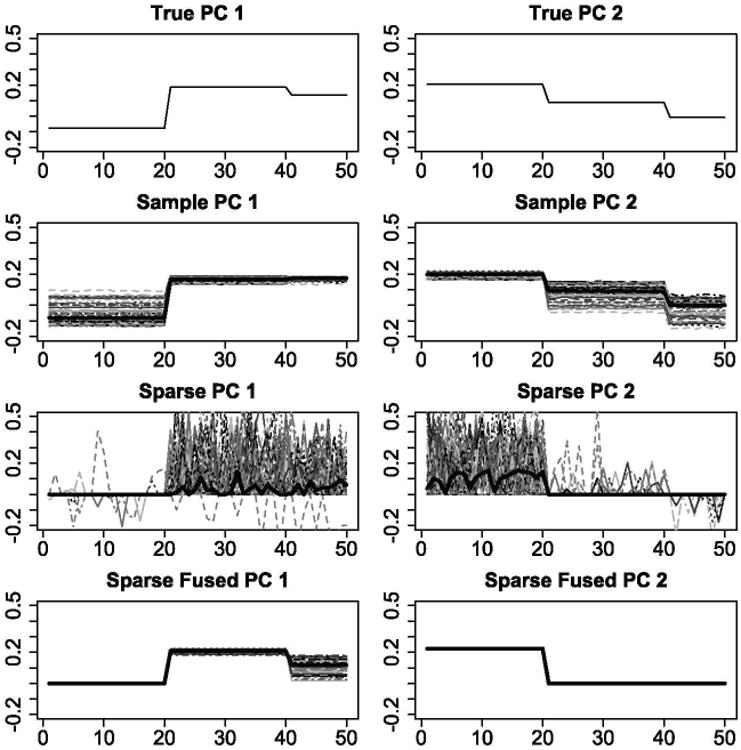
Factor loadings of the first (left column) and second (right column) PC vectors estimated by ordinary PCA from the true covariance (first row), ordinary PCA from the sample covariance (second row), sparse PCA (third row), and SFPCA (fourth row). The horizontal axis is the variables and the vertical axis is the value of the loadings. Each colored curve represents the PC vector in one replication. The median loadings over 50 repetitions are represented by the black bold lines. The online version of this figure is in color.
4. Application of SFPCA to Real Datasets
4.1 Drivers Dataset
This dataset provides information about the physical size and age of 38 drivers along with a response variable, seat position in a car (Faraway 2004). For the purposes of PCA, the response variable was excluded from the analysis. The eight available variables on driver characteristics are age, weight, height in shoes, height in bare feet, seated height, lower arm length, thigh length, and lower leg length. All height/length variables are highly correlated (average correlation among these variables is about 0.8) and form a natural block (Figure 2); hence, we expect them to have similar loadings. SFPCA was applied to this dataset and its results compared with those obtained from ordinary PCA and sparse PCA (Table 2).
Figure 2.
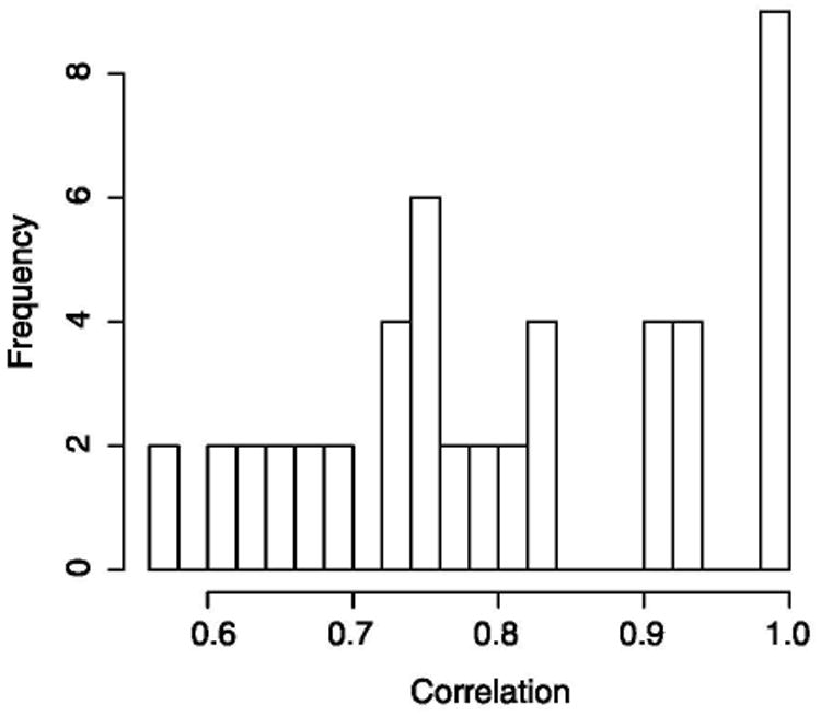
The histogram of the pairwise correlations between the height/length variables: weight, height in shoes, height in bare feet, seated height, lower arm length, thigh length, and lower leg length.
Table 2.
Numerical results for the drivers example.
| PC 1 | PC 2 | |||||
|---|---|---|---|---|---|---|
|
|
|
|||||
| Variables | PCA | SPCA | SFPCA | PCA | SPCA | SFPCA |
| Age | 0.007 | 0.876 | 0.970 | 1.000 | ||
| Weight | 0.367 | 0.284 | 0.378 | 0.045 | ||
| HtShoes | 0.411 | 0.139 | 0.378 | −0.106 | ||
| Ht | 0.412 | 0.764 | 0.378 | −0.112 | ||
| Seated | 0.381 | 0.313 | 0.378 | −0.218 | ||
| Arm | 0.349 | 0.208 | 0.378 | 0.374 | 0.242 | |
| Thigh | 0.328 | 0.247 | 0.378 | 0.125 | ||
| Leg | 0.390 | 0.341 | 0.378 | −0.056 | ||
| AV (96) | 70.9 | 55.0 | 68.7 | 15.5 | 14.2 | 12.2 |
| ACV (%) | 70.9 | 55.0 | 68.7 | 86.4 | 69.2 | 80.8 |
It can be seen that ordinary PCA captures the block structure in the first PC, but the factor loadings exhibit significant variation. Interestingly, the factor loadings from sparse PCA exhibit even greater variability, while the percentage of total variance explained by the first PC is only 55%, as opposed to 70% by ordinary PCA. On the other hand, SPFCA exhibits good performance in terms of goodness of fit (68.7%) and clearly reveals a single block structure in the “size” variables.
4.2 Pitprops Dataset
The pitprops dataset, introduced by Jeffers (1967), has become a classic example of the difficulties in interpretation of principal components. In this dataset, the sizes and properties of 180 pitprops (lumbers used to support the roofs of tunnels in coal mines) are recorded. The available variables are: the top diameter of the prop (topdiam), the length of the prop (length), the moisture content of the prop (moist), the specific gravity of the timber at the time of the test (testsg), the oven-dry specific gravity of the timber (ovensg), the number of annual rings at the top of the prop (ringtop), the number of annual rings at the base of the prop (ringbut), the maximum bow (bowmax), the distance of the point of maximum bow from the top of the prop (bowdist), the number of knot whorls (whorls), the length of clear prop from the top of the prop (clear), the average number of knots per whorl (knots), and the average diameter of the knots (diaknot). The first six PCs from regular PCA account for 87% of the total variability (measured by cumulative proportion of total variance explained).
We applied SPFCA and sparse PCA to the dataset and the results are given in Table 3. The loadings from SFPCA show a sparse structure similar to that of sparse PCA, but the first three PCs from SFPCA involve fewer variables than those of SPCA. The equal loadings within blocks assigned by SFPCA produce a clear picture for interpretation purposes. Referring to the interpretation of Jeffers (1967), the first PC gives the same loadings to “topdiam,” “length,” “ringbut,” “bowmax,” “bowdist,” and “whorls” and provides a general measure of size; the second PC assigns equal loadings to “moist” and “testsg” and measures the degree of seasoning; the third PC, giving equal loadings to “ovensg” and “ringtop,” accounts for the rate of the growth and the strength of the timber; the following three PCs represent “clear,” “knots,” and “diaknot,” respectively.
Table 3.
Numerical results for the pitprops example.
| PC 1 | PC 2 | PC 3 | |||||||
|---|---|---|---|---|---|---|---|---|---|
|
|
|
|
|||||||
| Variables | PCA | SPCA | SFPCA | PCA | SPCA | SFPCA | PCA | SPCA | SFPCA |
| topdiam | 0.404 | 0.477 | 0.408 | 0.218 | −0.207 | ||||
| length | 0.406 | 0.476 | 0.408 | 0.186 | −0.235 | ||||
| moist | 0.124 | 0.541 | 0.785 | 0.707 | 0.141 | ||||
| testsg | 0.173 | 0.456 | 0.620 | 0.707 | 0.352 | ||||
| ovensg | 0.057 | −0.177 | −0.170 | 0.481 | 0.640 | 0.707 | |||
| ringtop | 0.284 | 0.052 | −0.014 | 0.475 | 0.589 | 0.707 | |||
| ringbut | 0.400 | 0.250 | 0.408 | −0.190 | 0.253 | 0.492 | |||
| bowmax | 0.294 | 0.344 | 0.408 | −0.189 | -0.021 | -0.243 | |||
| bowdist | 0.357 | 0.416 | 0.408 | 0.017 | -0.208 | ||||
| whorls | 0.379 | 0.400 | 0.408 | −0.248 | -0.119 | ||||
| clear | −0.011 | 0.205 | -0.070 | ||||||
| knots | −0.115 | 0.343 | 0.013 | 0.092 | −0.015 | ||||
| diaknot | −0.113 | 0.309 | −0.326 | −0.308519 | |||||
| AV (%) | 32.4 | 28.0 | 31.5 | 18.3 | 14.4 | 15.1 | 14.4 | 13.3 | 10.1 |
| ACV (%) | 32.4 | 28.0 | 31.5 | 50.7 | 42.0 | 46.6 | 65.1 | 55.3 | 56.7 |
| PC 4 | PC 5 | PC 6 | |||||||
|
|
|
|
|||||||
| topdiam | −0.091 | 0.083 | 0.120 | ||||||
| length | −0.103 | 0.113 | 0.163 | ||||||
| moist | 0.078 | −0.350 | −0.276 | ||||||
| testsg | 0.055 | −0.356 | −0.054 | ||||||
| ovensg | 0.049 | −0.176 | 0.626 | ||||||
| ringtop | -0.063 | 0.316 | 0.052 | ||||||
| ringbut | −0.065 | 0.215 | 0.003 | ||||||
| bowmax | 0.286 | −0.185 | −0.055 | ||||||
| bowdist | 0.097 | 0.106 | 0.034 | ||||||
| whorls | −0.205 | −0.156 | −0.173 | ||||||
| clear | 0.804 | 1.000 | 1.000 | 0.343 | 0.175 | ||||
| knots | −0.301 | 0.600 | 1.000 | 1.000 | −0.170 | ||||
| diaknot | −0.303 | −0.08 | 0.626 | 1.000 | 1.000 | ||||
| AV (%) | 8.5 | 7.4 | 8.0 | 7.0 | 6.8 | 7.3 | 6.3 | 6.2 | 7.0 |
| ACV (%) | 73.6 | 62.7 | 64.7 | 80.6 | 69.5 | 72.0 | 86.9 | 75.8 | 79.0 |
4.3 Meat Spectrum Data
In this section, we apply SFPCA to a dataset involving spectra obtained from meat analysis (Borggaard and Thodberg 1992; Thodberg 1996). In recent decades, spectrometry techniques have been widely used to identify the fat content in pork, because it has proved significantly cheaper and more efficient than traditional analytical chemistry methods. In this dataset, 215 samples were analyzed by a Tecator near-infrared spectrometer which measured the spectrum of light transmitted through a sample of minced pork meat. The spectrum gives the absorbance at 100 wavelength channels in the range of 850 to 1050 nm.
The adjusted cumulative total variances explained by the first two PCs from ordinary PCA, sparse PCA, and SFPCA are 99.6%, 98.9%, and 98.4%, respectively. Since wavelengths are naturally ordered, a natural way to display the loadings is to plot them against the wavelength. The plot of the first two PCs for the 100 wavelength channels is shown in Figure 3.
Figure 3.
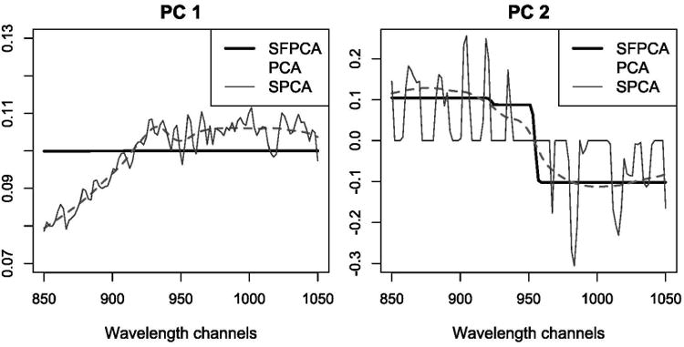
Comparison of the first (left panel) and second (right panel) PC vectors from ordinary PC A (dashed line), sparse PCA (dotted line), and SFPCA (solid line). The online version of this figure is in color.
SFPCA smooths the ordinary PC vectors producing piecewise linear curves which are easier to interpret. The SFPCA results show clearly that the first PC represents the overall mean over different wavelengths while the second PC represents a contrast between the low and high frequencies. On the other hand, the high variability in the loadings produced by sparse PCA makes the PC curves difficult to interpret.
4.4 USPS Handwritten Digit Data
In this example, the three PCA methods are compared on the USPS handwritten digit dataset (Hull 1994). This dataset was collected by the U.S. Postal Service (USPS) and contains 11,000 gray scale digital images of the ten digits at 16 × 16 pixel resolution. We focused on the digit “3” and sampled 20 images at random, thus operating in a large p, small n setting. While BIC gave good results for most datasets we examined, for the USPS data it tended to undershrink the coefficient estimates. However, we found that cross-validation produced good results and was computationally feasible, so we used 5-fold cross-validation to select the optimal tuning parameters for SPCA and SFPCA. The optimal tuning parameter for SPCA turned out to be equal to zero, so here SPCA coincides with ordinary PCA. The reconstructed images by the first and second principal components (“eigenimages”) arranged in the original spatial order are shown in Figure 4. It can be seen that SFPCA achieves a fairly strong fusing effect for the background pixels, thus producing a smoother, cleaner background image. This is confirmed by the results in Table 4 that give the proportion of distinct elements in the first two principal components for PCA and SFPCA. Notice that since PCA does not impose any sparsity or fusion, the resulting proportion is 100%, compared to those for SFPCA (35.5% and 22.7% for the first and second PCs, respectively).
Figure 4.
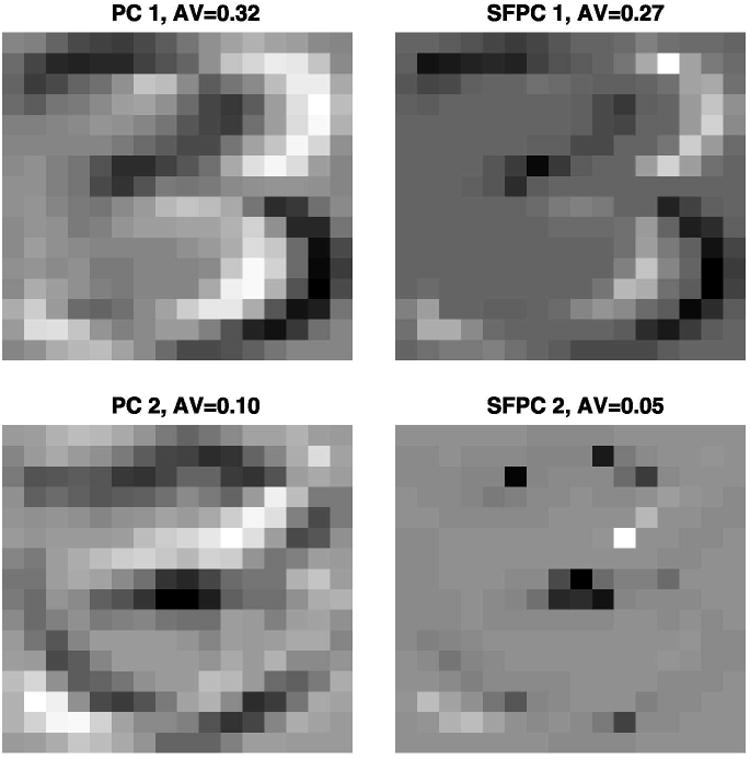
The first two eigenimages of digit “3” estimated by PCA and SFPCA, respectively.
Table 4.
The proportion of distinct elements in the eigenimages of digit “3” estimated by PCA and SFPCA, respectively.
| PC | PCA (%) | SFPCA (%) |
|---|---|---|
| 1 | 100 | 35.5 |
| 2 | 100 | 22.7 |
5. Concluding Remarks
In this article, a method is developed to estimate principal components that capture block structures in the variables, which aids in the interpretation of the data analysis results. To achieve this goal, the orthogonality requirement is relaxed and an ℓ1 penalty is imposed on the norm of the PC vectors, as well as a “fusion” penalty driven by variable correlations. Application of the method to both synthetic and real datasets illustrates its advantages when it comes to interpretation.
The idea of sparse fused loadings is also applicable in a number of other unsupervised learning techniques, including canonical correlation and factor analysis, as well as regression analysis, classification techniques (e.g., LDA and SVM), and survival analysis (e.g., Cox model and Buckley–James model). We note that Daye and Jeng (2009) proposed a weighted fusion penalty for variable selection in a regression model. Unlike the generalized fusion penalty which penalizes the pairwise Manhattan distances between the variables, their method penalizes the pairwise Euclidean distances, and thus would not necessarily shrink the coefficients of highly correlated variables to identical values. Similarly, Tutz and Ulbricht (2009) proposed a BlockBoost method, whose penalty also tends to fuse the pairwise difference between the regression coefficients. In particular, when these pairwise correlations are close to ±1, the solution of BlockBoost is close to that of Daye and Jeng (2009).
Supplementary Material
Acknowledgments
The authors thank the editor, David van Dyk, the associate editor, and two referees for helpful comments and suggestions. E. Levina's research was partially supported by NSF grants DMS-0505424 and DMS-0805798. G. Michailidis's research was partially supported by NIH grant 1RC1CA145444-0110 and MEDC grant GR-687. J. Zhu's research was partially supported by NSF grants DMS-0505432, DMS-0705532, and DMS-0748389.
Footnotes
Supplemental Materials: Supplemental Figure: This figure contains the histograms of pairwise angles between the first four PC vectors estimated by SFPCA in this simulation, (supplementalfigure.pdf)
R-code: The R code (sfpca.R) implementing the algorithm of SFPCA and a Readme file (readme.pdf) to show how to use it. (R-code.zip)
Datasets: All datasets (digit0to9.Rdat) used in this article, as well as a Readme file (Readme.rtf). (Datasets.zip)
Contributor Information
Jian Guo, Email: guojian@umich.edu, Department of Statistics, University of Michigan, 269 West Hall, 1085 South University Avenue, Ann Arbor, MI 48109-1107.
Gareth James, Email: gareth@usc.edu, Marshall School of Business, University of Southern California, Los Angeles, CA 90089-0809.
Elizaveta Levina, Email: elevina@umich.edu, University of Michigan, 459 West Hall, 1085 South University Avenue, Ann Arbor, MI 48109-1107.
George Michailidis, Email: gmichail@umich.edu, University of Michigan, 459 West Hall, 1085 South University Avenue, Ann Arbor, MI 48109-1107.
Ji Zhu, Email: jizhu@umich.edu, University of Michigan, 459 West Hall, 1085 South University Avenue, Ann Arbor, MI 48109-1107.
References
- Bazaraa M, Sherali H, Shetty C. Nonlinear Programming: Theory and Algorithms. New York: Wiley; 1993. 936. [Google Scholar]
- Borggaard C, Thodberg H. Optimal Minimal Neural Interpretation of Spectra. Analytic Chemistry. 1992;64:545–551. 941. [Google Scholar]
- Daye Z, Jeng X. Shrinkage and Model Selection With Correlated Variables via Weighted Fusion. Computational Statistics and Data Analysis. 2009;53:1284–1298. 943,944. [Google Scholar]
- Fan J, Li R. Variable Selection via Nonconcave Penalized Likelihood and Its Oracle Properties. Journal of the American Statistical Association. 2001;96:1348–1360. 934,935. [Google Scholar]
- Faraway J. Linear Model in R. Boca Raton, FL: CRC Press; 2004. 940. [Google Scholar]
- Hull J. A Database for Handwritten Text Recognition Research. IEEE Transactions on Pattern Analysis and Machine Intelligence. 1994;16:550–554. 942. [Google Scholar]
- Hunter D, Li R. Variable Selection Using MM Algorithms. The Annals of Statistics. 2005;33:1617–1642. doi: 10.1214/009053605000000200. 935,936. [DOI] [PMC free article] [PubMed] [Google Scholar]
- Jeffers J. Two Cases Studies in the Application of Principal Component. Applied Statistics. 1967;16:225–236. 940,941. [Google Scholar]
- Jollife I. Rotation of Principal Components: Choice of Normalization Constraints. Journal of Applied Statistics. 1995;22:29–35. 931. [Google Scholar]
- Jollife I, Trendafilov N, Uddin M. A Modified Principal Component Technique Based on the LASSO. Journal of Computational and Graphical Statistics. 2003;12:531–547. 931,932. [Google Scholar]
- Land S, Friedman J. technical report. Stanford University, Dept. of Statistics; Stanford: 1996. Variable Fusion: A New Method of Adaptive Signal Regression. 934. [Google Scholar]
- Li C, Li H. Network-Constraint Regularization and Variable Selection for Analysis of Genomic Data. Bioinformatics. 2008;24:1175–1182. doi: 10.1093/bioinformatics/btn081. 934. [DOI] [PubMed] [Google Scholar]
- McCabe G. Principal Variables. Technometrics. 1984;26:137–144. 931. [Google Scholar]
- Thodberg H. A Review of Bayesian Neural Networks With an Application to Nearinfrared Spectroscopy. IEEE Transactions on Neural Networks. 1996;7:56–72. doi: 10.1109/72.478392. 941. [DOI] [PubMed] [Google Scholar]
- Tibshirani R, Saunders M, Rosset S, Zhu J, Knight K. Sparsity and Smoothness via the Fused Lasso. Journal of the Royal Statistical Society, Ser B. 2005;67:91–108. 934,936. [Google Scholar]
- Tutz G, Ulbricht J. Penalized Regression With Correlation-Based Penalty. Statistics and Computing. 2009;19:239–253. 944. [Google Scholar]
- Vines S. Simple Principal Components. Applied Statistics. 2000;49:441–451. 931. [Google Scholar]
- Zou H, Hastie T. Regularization and Variable Selection via the Elastic Net. Journal of the Royal Statistical Society, Ser B. 2005;67:301–320. 931. [Google Scholar]
- Zou H, Hastie T, Tibshirani R. Sparse Principal Component Analysis. Journal of Computational and Graphical Statistics. 2006;15:265–286. 931-934,937. [Google Scholar]
- Zou H, Hastie T, Tibshirani R. On the Degrees of Freedom of the LASSO. The Annals of Statistics. 2007;35:2173–2192. 936. [Google Scholar]
Associated Data
This section collects any data citations, data availability statements, or supplementary materials included in this article.