Calibrated Birth–Death Phylogenetic Time-Tree Priors for Bayesian Inference

Abstract

Here we introduce a general class of multiple calibration birth–death tree priors for use in Bayesian phylogenetic inference. All tree priors in this class separate ancestral node heights into a set of “calibrated nodes” and “uncalibrated nodes” such that the marginal distribution of the calibrated nodes is user-specified whereas the density ratio of the birth–death prior is retained for trees with equal values for the calibrated nodes. We describe two formulations, one in which the calibration information informs the prior on ranked tree topologies, through the (conditional) prior, and the other which factorizes the prior on divergence times and ranked topologies, thus allowing uniform, or any arbitrary prior distribution on ranked topologies. Although the first of these formulations has some attractive properties, the algorithm we present for computing its prior density is computationally intensive. However, the second formulation is always faster and computationally efficient for up to six calibrations. We demonstrate the utility of the new class of multiple-calibration tree priors using both small simulations and a real-world analysis and compare the results to existing schemes. The two new calibrated tree priors described in this article offer greater flexibility and control of prior specification in calibrated time-tree inference and divergence time dating, and will remove the need for indirect approaches to the assessment of the combined effect of calibration densities and tree priors in Bayesian phylogenetic inference.

Divergence time dating and phylogenetic inference are related concerns. Recent advances in Bayesian phylogenetic inference (Rannala and Yang 1996; Yang and Rannala 1997; Huelsenbeck and Ronquist 2001; Drummond and Rambaut 2007) have culminated in the field of relaxed phylogenetic inference, in which both divergence times and phylogenetic relationships are simultaneously estimated (Drummond et al. 2006). This estimation is aided by relaxed molecular clocks (Thorne et al. 1998; Kishino et al. 2001; Thorne and Kishino 2002; Drummond et al. 2006; Rannala and Yang 2007) which reconcile nonclock-like evolution with an underlying time-tree in which common ancestors are placed on an axis of time. To produce results on an absolute time scale it is necessary to either provide information on the rate of molecular evolution or alternatively calibrate a subset of internal nodes with a calibration density (Thorne et al. 1998; Drummond et al. 2006; Yang and Rannala 2006). Either way, in a Bayesian setting, a tree prior must also be placed on all the uncalibrated divergence times. The tree prior is a function that assigns a prior probability density to every possible tree. Arguably the simplest tree priors are the one-parameter Yule model (Yule 1924) and the two-parameter birth–death model (Nee et al. 1994; Gernhard 2008). The latter has been suggested as an appropriate null model for species diversification Nee et al. (1994a) and has been extended to include additional parameters to model various types of incomplete sampling (Yang and Rannala 1997; Stadler 2009b; Höhna et al. 2011). The other commonly used tree prior, the coalescent (Kingman 1982), is typically deployed when all the samples are from the same species. The coalescent is not handled here but calibration information for a specific group of individuals usually does not exist. However, the calibrated prior can be used to calibrate a species tree, within which the gene trees follow the “multispecies coalescent” prior in a species-tree/gene-trees analysis (Heled and Drummond 2010).

In a Bayesian setting, combining a calibration density (on one or more divergences) with a tree prior into a single calibrated tree prior for divergence time estimation possesses a number of subtleties worthy of note, which we cover under the following headings.

Fossil Bounds on a Single Divergence

Consider the simplest type of calibration to admit uncertainty: The placement of an upper and a lower limit on the age of a single divergence ($h_C$) in the tree:

$${\rho }_h(h_C)=\{\begin{array}{cc}1/(u-l)& l\le h_C\le u\\ 0& \text{otherwise}\end{array}$$ (1)

A node calibration of this type is associated with a specific subset of the taxa $C$. Throughout this article our analytical results and implementations require that these taxa are monophyletic in the phylogeny, and their most recent common ancestor is the divergence that is calibrated. The topology within the calibrated clade can be subject to uncertainty, as can the topology outside the calibrated clade, but the existence of the clade is a condition of the calibration.

This simple approach to calibration already has two quite distinct interpretations in a Bayesian setting when considered within the context of an overall tree prior on all divergence times. One interpretation is that the resulting marginal prior distribution on the calibrated divergence should obey the tree prior (e.g., Yule or birth–death) but be constrained to be within the upper and lower bounds, so that the full calibrated tree prior, ${\rho }_G(·)$, is:

$${\rho }_G(h,\psi |\Lambda )\propto f_G(h,\psi |\Lambda ){\rho }_h(h_C),$$ (2)

where $h$ represents the set of all divergence times, $\psi$ is the ranked tree topology and $\Lambda$ represents the parameter(s) of the tree prior. The interpretation above was the only one available in the BEAST software until recently (Heled and Drummond 2012). An alternative “conditional-on-calibrated-node-ages” interpretation is that the marginal prior on the calibrated divergence should be uniform between the upper and lower limits and the prior on the remaining divergence times should follow the tree process prior, $f_G(h,\psi |\Lambda )$, conditioned on the height of the calibrated node (Yang and Rannala 2006):

$${\rho }_G(h,\psi |\Lambda )=f_G(h\setminus h_C,\psi |\Lambda ){\rho }_h(h_C),$$ (3)

There is a difference between these two prior formulations regardless of whether the tree topology is known or estimated. In a previous work Heled and Drummond (2012) described how to efficiently compute the latter formulation in the face of uncertainty in tree topology for arbitrary single-divergence calibration densities under the Yule tree prior.

Nested Calibrations

It has been routine in almost all treatments of phylogenetic calibration so far to specify independent univariate priors for each calibrated divergence time. However, calibrated divergence times that are nested in the tree are necessarily interdependent, such that the more recent calibrated divergence of a nested pair must be younger than the older calibrated divergence. If the specified calibration densities overlap then the resulting marginals of the joint prior will necessarily differ from the specified calibration densities. We do not address this issue here. However, the correct solution to this problem is simply to specify a joint prior on the calibrated nodes that obeys the necessary condition that nested nodes are order statistics and, therefore, not free to vary independently.

The Influence of Calibrations on the Tree Topology Prior

Heled and Drummond (2012) demonstrated that a natural interpretation of the “conditional-on-calibrated-age” construction of a calibrated tree prior produces a distribution that is non-uniform on ranked topologies. However, we show in this article that the tree prior can be decomposed into a prior on the node ages (both calibrated and uncalibrated) and a prior on the set of possible ranked histories. We show that this provides a means to compute a tree prior rapidly if a uniform prior on ranked trees is chosen. We compare this approach to a computational intensive alternative that weighs each ranked tree topology by its probability conditional on the divergence times of the calibrated nodes. The latter is a natural extension to our previous work to the case of multiple calibrations and a birth–death process prior. However, this extension turns out to be computationally expensive except for some special cases where a closed-form formula exists. We therefore advocate the former approach (that always applies a uniform prior to ranked trees) as a practical alternative.

Methods

Consider the following notation:

• $n$ Number of taxa.

• $\Psi$ The set of all ranked binary topologies on $n$ taxa. We keep $n$ implicit to simplify the notation.

• $\psi$ A ranked tree ($\psi \in \Psi$). See Gavryushkina et al. (2013) for a formal definition of a ranked tree.

• $h=\{h_1,h_2,\cdots ,h_{n-1}:h_i\ge h_{i+1}\ge 0\}$, an ordered set of divergence ages.

• $g=\langle h,\psi \rangle$, a time tree on $n$ taxa.

• $G$ the space of all time trees.

• $\Lambda$ the parameters of the tree prior process. For the pure birth (Yule) prior $\Lambda =\{\lambda \}$, where $\lambda$ is the birth rate, while $\Lambda =\{\lambda ,\mu ,\rho \}$ for the birth–death prior, where $\mu$ is the death rate and $\rho$ is the sampling rate.

• $\theta =\langle \Omega ,R\rangle$, a pair of parameter vectors, one for the substitution process $\Omega$ and one for the rates of the molecular clock, $R$.

Posterior Probability for Bayesian Inference

Without calibration, the posterior probability density of $(g,\Lambda ,\theta )$ given a sequence alignment, $D$ can be written:

$$f(g,\Lambda ,\theta |D)=\frac{Pr\{D|g,\theta \}f(\theta )f_G(g|\Lambda )f(\Lambda )}{Pr\left\{D\right\}}.$$ (4)

The term $Pr\{D|g,\theta \}$ is the phylogenetic likelihood (Felsenstein 1981). The rates $R$ and divergence times $h$ combine to provide branch lengths in units of substitutions per site on the edges of $\psi$. The term $f_G(g|\Lambda )$ is the uncalibrated tree prior and it can be readily factored in the following way:

$$f_G(g|\Lambda )=f(h|\Lambda )\mathrm{Pr}(\psi |\Lambda ).$$ (5)

$f(h|\Lambda )$ is easy to compute for the pure birth (Yule) prior, birth–death prior or any prior whose equivalence classes are defined entirely by the divergence time order statistics. Under the Yule or birth–death prior without calibrations, $\mathrm{Pr}(\psi |\Lambda )=|\Psi {|}^{-1}$, is a uniform prior on all ranked topologies. However, this factorization is no longer simple when calibrations are introduced (Heled and Drummond 2012), and so we must develop an alternative approach to describing the calibrated tree prior in the following sections, which we will call ${\rho }_G(·)$ to distinguish from the uncalibrated tree prior $f_G(·)$. Note that throughout the remaining sections the tree priors are always conditional on $\Lambda$, but we suppress the conditioning in the notation for the sake of clarity.

Calibrated Birth–Death Density

We introduce some extra notation for calibrations:

• $K$ Number of calibration points.

• $\phi$ Set of conditions on $\Psi$, typically clade monophyly constraints. $\phi$ plays a part in the terms defined below, but because it is fixed in each case we mostly keep it implicit to make the equations easier to read.

• ${\Psi }_{\phi }$ The subset of all ranked topologies for which $\phi$ holds.

• $i(\psi )=(i_1,i_2,\cdots ,i_K)$, mapping a ranked tree to the ranks of the calibrated nodes. Typically those are the ranks of the clades in $\phi$, but $i$ may, for example, pick the rank of a clade's parent instead.

  We use two additional mappings which are a function of $i$. $\overline{i}(\psi )=({\overline{i}}_1,{\overline{i}}_2,\cdots ,{\overline{i}}_K)$ is the mapping of calibration ranks into their sort order. For example, if $i=(3,1,4)$ then $\overline{i}=(2,1,3)$ and if $i=(7,4,2)$ then $\overline{i}=(3,2,1)$.

  Also, $\hat{i}(\psi )=({\hat{i}}_1,{\hat{i}}_2,\cdots ,{\hat{i}}_K)=(i_{\overline{i}1},i_{\overline{i}2},\cdots ,i_{\overline{i}K})$ are the ranks of the calibrated nodes sorted by age. For the two examples above we have, respectively, $\hat{i}=(1,3,4)$ and (2,4,7).

• ${\Psi }_{\phi ,x}$ The subset of $\psi \in {\Psi }_{\phi }$ for which $\overline{i}(\psi )$ is equal to the sorting order of the heights vector $x$. That is, all the ranked topologies which are compatible with the heights $x$.

• $h_{\psi }=(h_{i_1},h_{i_2},\cdots ,h_{i_K})$, the heights of the calibration points on a given ranked tree $\psi$. For convenience $g_{\psi }$ is the same as $h_{\psi }$ when $g=\langle h,\psi \rangle$.

• ${\rho }_h(h_{\psi })$ A $K$-dimensional calibration density.

Figure 1 illustrates the main elements of our notation on an example tree with seven taxa and three calibrated subclades.

Figure 1.

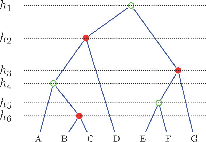
Notation. For the tree depicted we have: $n=7$ taxa, the ranked topology $\psi$ = (((a,(b,c):1):3,d):5,((e,f):2,g):4) in NEWICK format, with internal nodes marked by rank, $\phi$ = ({e,f,g}, {b,c}, {a,b,c,d}), $K=3$ calibrated nodes marked in red, and $i(\psi )=(3,6,2)$, $\overline{i}(\psi )=(3,1,2)$, $\hat{i}(\psi )=(2,3,6)$ and $h_{\psi }=(h_3,h_6,h_2)$.

In BEAST, the calibrated tree prior has been defined as,

$${\rho }_G^{(M)}(g)\equiv f_G(g){\rho }_h(h_{\psi }).$$ (6)

We shall call this the multiplicative prior, as designated by the superscript (M). While multiplying the two densities create some valid (unnormalized) prior density, this tree prior fails to preserve the calibration density as the marginal prior distribution of the calibrated nodes. That is, the marginal calibration density—the density obtained by integrating out the non-calibrated heights over all time trees—is not equal to ${\rho }_h$.

In Heled and Drummond (2012) we showed that it is easy in principle to preserve the calibration marginal by scaling the prior with the conditional marginal value, that is, the total density of all trees whose calibration times are identical to the calibration times of $g$:

$$f_h(x)={\displaystyle \underset{\begin{array}{c}g\in G\\ g_{\psi }=x\end{array}}{\int }{f}_G}(g)\text{d}g.$$ (7)

The same general principle works for multiple calibrations:

$${\rho }_G(g)\equiv f_G(g)\frac{{\rho }_h(h_{\psi })}{f_h(h_{\psi })}.$$ (8)

The notation for describing the calibrated prior is challenging because calibrated clade ages are not a simple subset of all ages. It may seem natural to define the joint density by defining the tree prior density as the product of conditional and calibration priors as done in Equation 3 of (Yang and Rannala 2006) and mirrored in our own Equation 3. But then Yang and Rannala deal only with trees whose ranked topology is known. For example, with this formulation one can easily forget that the space of possible values for the uncalibrated nodes depends on the tree topology and the calibrated nodes, and although this notational omission may be fine when the topology is fixed, it should be explicit when dealing with the whole of tree space. We think our notation is better suited for describing the properties of the prior in the context of the full tree space.

The conditional prior in equation (8) preserves the marginal by construction. This is easy to see by writing down the marginal density for $x$, a fixed vector of calibration values:

$$\begin{array}{l}{\displaystyle \underset{\begin{array}{c}g\in G\\ h_{\psi }=x\end{array}}{\int }{f}_G}(g)\frac{{\rho }_h(h_{\psi })}{f_h(h_{\psi })}\text{d}g={\displaystyle \underset{\begin{array}{c}g\in G\\ h_{\psi }=x\end{array}}{\int }{f}_G}(g)\frac{{\rho }_h(x)}{f_h(x)}\text{d}g={\rho }_h(x)\hspace{0.17em}\hspace{0.17em}\frac{{\displaystyle \underset{\begin{array}{c}g\in G\\ h_{\psi }=x\end{array}}{\int }{f}_G}(g)\text{d}g}{f_h(x)}\\ ={\rho }_h(x).\end{array}$$ (9)

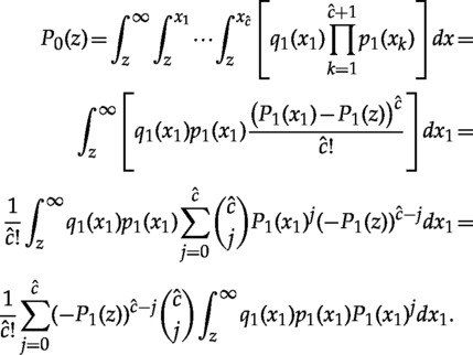
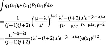
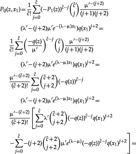
However, the usefulness of this prior depends upon the computational cost of evaluating $f_h(x)$ as part of the full posterior. In a few cases we can obtain a simple formula and the cost is negligible, and for the rest we offer either (i) a general algorithm for computing the marginal by iteration or (ii) the restricted conditional, a faster alternate correction to be used when (i) is too slow. The iterative approach is based upon the clade level partition, which divides ${\Psi }_{\phi }$ into disjoint subgroups whose marginal has a closed form, and we shall discuss the details later.

The restricted conditional prior is defined as follows

$${\rho }_G^{(R)}(g=\langle \psi ,h\rangle )\equiv f_G(g)\frac{{\rho }_h(h_{\psi })}{f_h^{(R)}(h_{\psi },\psi )},$$ (10)

where

$$f_h^{(R)}(x,\psi )=|{\Psi }_{\phi ,x}|{\displaystyle \underset{h_{\psi }=x}{\int }{f}_G}(\langle \psi ,h\rangle )\text{d}h.$$ (11)

Here the correction is defined as the marginal of the tree prior density when keeping both the topology and calibrated ages fixed. This is equivalent to extending the approach taken by Yang and Rannala (2006) to the case of an unknown tree topology. Again, the marginal over tree space is preserved by construction,

$$\begin{array}{l}{\displaystyle \underset{\begin{array}{c}g=\langle \psi ,h\rangle \in G\\ h_{\psi }=x\end{array}}{\int }{f}_G}(g)\frac{{\rho }_h(h_{\psi })}{f_h^{(R)}(h_{\psi },\psi )}\text{d}g={\displaystyle \sum _{\psi \in {\Psi }_{\phi ,x}}\hspace{0.17em}}\hspace{0.17em}{\displaystyle \underset{\begin{array}{c}g=\langle \psi ,h\rangle \\ h_{\psi }=x\end{array}}{\int }{f}_G}(g)\frac{{\rho }_h(x)}{f_h^{(R)}(x,\psi )}\text{d}h=\\ {\rho }_h(x){\displaystyle \sum _{\psi \in {\Psi }_{\phi ,x}}\hspace{0.17em}}\hspace{0.17em}\frac{1}{f_h^{(R)}(x,\psi )}{\displaystyle \underset{\begin{array}{c}g=\langle \psi ,h\rangle \\ h_{\psi }=x\end{array}}{\int }{f}_G(g)}\text{d}h={\rho }_h(x){\displaystyle \sum _{\psi \in {\Psi }_{\phi }}\frac{1}{|{\Psi }_{\phi ,x}|}}={\rho }_h(x).\end{array}$$ (12)

The Marginal Yule for Multiple Calibrations

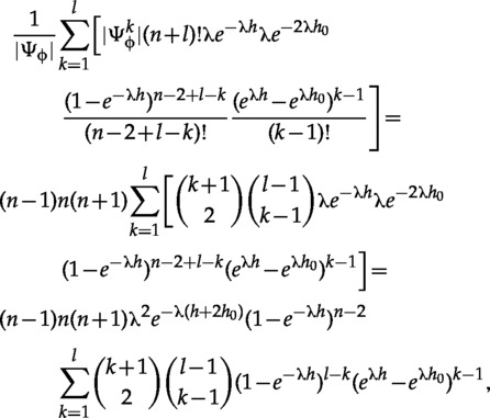
We start by showing how to decompose the Yule density of genealogy $g=\langle \psi ,h\rangle$ conditional on $\phi$. The decomposition is based on separating the heights into $K+1$ levels, where each level spans the range between two consecutive calibration points.

The Yule density

$$f_G(h|\lambda )=\frac{1}{|{\Psi }_{\phi }|}n!e^{-\lambda h_1}{\displaystyle \prod _{i=1}^{n-1}\lambda }{e}^{-\lambda h_i}$$ (13)

is factored using the two propositions below.

• Proposition I:

  $$\begin{array}{l}{\displaystyle {\int }_a^b\text{d}{x}_1}{\displaystyle {\int }_a^{x_1}\text{d}{x}_2}{\displaystyle {\int }_a^{x_2}\text{d}{x}_3}\cdots {\displaystyle {\int }_a^{x_{k-1}}\text{d}{x}_k}\hspace{0.17em}\hspace{0.17em}\lambda e^{-\lambda x_1}\lambda e^{-\lambda x_2}\cdots \lambda e^{-\lambda x_k}=\\ \frac{1}{k!}\left[{\displaystyle {\int }_a^b\lambda }{e}^{-\lambda x_1}\text{d}{x}_1\right]\left[{\displaystyle {\int }_a^b\lambda }{e}^{-\lambda x_2}\text{d}{x}_2\right]\cdots \left[{\displaystyle {\int }_a^b\lambda }{e}^{-\lambda x_k}\text{d}{x}_k\right]=\\ \frac{1}{k!}{\left(e^{-\lambda b}-e^{-\lambda a}\right)}^k\end{array}$$ (14)
• Proposition II:

  $$\begin{array}{l}{\displaystyle {\int }_a^{\infty }\text{d}{x}_0}{\displaystyle {\int }_a^{x_0}\text{d}{x}_1}{\displaystyle {\int }_a^{x_1}\text{d}{x}_2}\cdots {\displaystyle {\int }_a^{x_{k-1}}\text{d}{x}_k}\hspace{0.17em}\hspace{0.17em}\lambda e^{-2\lambda x_0}\lambda e^{-\lambda x_1}\cdots \lambda e^{-\lambda x_k}\\ \text{by proposition I}\\ ={\displaystyle {\int }_a^{\infty }\lambda }{e}^{-2\lambda x_0}\frac{1}{k!}{\left(e^{-\lambda a}-e^{-\lambda x_0}\right)}^k\text{d}{x}_0\\ \text{by}\hspace{0.17em}\text{Equation}\hspace{0.17em}(\text{A}.\text{10)}\\ =\frac{1}{(k+2)!}{e}^{-(k+2)\lambda a}.\end{array}$$ (15)

Proposition I gives the contribution of $k$ internal nodes located between two consecutive calibration points with ages $a$ and $b$. Proposition II gives the contribution of $k+1$ nodes older than the last calibration point.

When the calibration values are fixed to $x=(x_1,x_2,\cdots ,x_K)$, the contribution of the ranked topology $\psi$ is

$$\begin{array}{l}{f}_h(x,\psi )={\displaystyle {\int }_{{\overline{x}}_1}^{\infty }\text{d}}{h}_1{\displaystyle {\int }_{{\overline{x}}_1}^{h_1}\text{d}}{h}_2\cdots {\displaystyle {\int }_{{\overline{x}}_1}^{h_{{\hat{i}}_1-3}}\text{d}}{h}_{{\hat{i}}_1-2}{\displaystyle {\int }_{{\overline{x}}_1}^{h_{{\hat{i}}_1-2}}\text{d}}{h}_{{\hat{i}}_1-1}\\ {\displaystyle {\int }_{{\overline{x}}_2}^{{\overline{x}}_1}\text{d}}{h}_{{\hat{i}}_1+1}{\displaystyle {\int }_{{\overline{x}}_2}^{h_{{\hat{i}}_1+1}}\text{d}}{h}_{{\hat{i}}_1+2}\cdots {\displaystyle {\int }_{{\overline{x}}_2}^{h_{{\hat{i}}_2-3}}\text{d}}{h}_{{\hat{i}}_2-2}\\ {\displaystyle {\int }_{{\overline{x}}_2}^{h_{{\hat{i}}_2-2}}\text{d}}{h}_{{\hat{i}}_2-1}{\displaystyle {\int }_{{\overline{x}}_3}^{{\overline{x}}_2}\text{d}}{h}_{{\hat{i}}_2+1}{\displaystyle {\int }_{{\overline{x}}_3}^{h_{{\hat{i}}_2+1}}\text{d}}{h}_{{\hat{i}}_2+2}\cdots \\ {\displaystyle {\int }_{{\overline{x}}_3}^{h_{{\hat{i}}_3-3}}\text{d}}{h}_{{\hat{i}}_3-2}{\displaystyle {\int }_{{\overline{x}}_3}^{h_{{\hat{i}}_3-2}}\text{d}}{h}_{{\hat{i}}_3-1}\\ \cdots \\ {\displaystyle {\int }_0^{{\overline{x}}_K}\text{d}{h}_{{\hat{i}}_{K+1}}}{\displaystyle {\int }_0^{h_{{\hat{i}}_{K+1}}}\text{d}{h}_{{\hat{i}}_{K+2}}}\cdots {\displaystyle {\int }_0^{h_3}\text{d}}{h}_{n-2}\\ {\displaystyle {\int }_0^{h_2}\text{d}}{h}_{n-1}{f}_G(\langle \psi ,h\rangle ).\end{array}$$ (16)

The above uses $\overline{x}=(x_{{\overline{i}}_1},x_{{\overline{i}}_2},\cdots ,x_{{\overline{i}}_K})$, the calibration height sorted by age. Now, let $c_j$ be the number of internal nodes in each level, $c_j={\hat{i}}_{j+1}-{\hat{i}}_j-1\hspace{0.17em}\hspace{0.17em}(0\le j\le K)$, and for convenience let ${\hat{i}}_0=0$ and ${\hat{i}}_{K+1}=n$. Using Propositions I and II we get

$$\begin{array}{l}{f}_h(x,\psi )=\frac{n!}{|{\Psi }_{\phi }|}\frac{e^{-(c_0+1)\lambda {\overline{x}}_1}}{(c_0+1)!}\\ \frac{\lambda e^{-\lambda {\overline{x}}_1}}{c_1!}{\left(e^{-\lambda {\overline{x}}_2}-e^{-\lambda {\overline{x}}_1}\right)}^{c_1}\\ \frac{\lambda e^{-\lambda {\overline{x}}_2}}{c_2!}{\left(e^{-\lambda {\overline{x}}_3}-e^{-\lambda {\overline{x}}_2}\right)}^{c_2}\\ \cdots \\ \frac{\lambda e^{-\lambda {\overline{x}}_K}}{c_{K!}}{\left(e^{-0}-e^{-\lambda {\overline{x}}_K}\right)}^{c_K}\\ =\left[\frac{n!}{|{\Psi }_{\phi }|}{\displaystyle \prod _{k=1}^K\lambda e^{-\lambda {\overline{x}}_k}}\right]\frac{e^{-(c_0+1)\lambda {\overline{x}}_1}}{(c_0+1)!}\\ {\displaystyle \prod _{k=1}^K\frac{{\left(e^{-\lambda {\overline{x}}_{k+1}}-e^{-\lambda {\overline{x}}_k}\right)}^{c_k}}{c_k!}}.\end{array}$$ (17)

The marginal density is the sum over all valid topologies

$$f_h(x)={\displaystyle \sum _{\begin{array}{c}\psi \in {\Psi }_{\phi }\\ \overline{i}(\psi )=\overline{i}(x)\end{array}}{f}_h}(x,\psi ).$$ (18)

To be valid, the order of calibration points by age has to be compatible with $x$.

While explicitly summing over all topologies is not feasible, evaluating the sum is possible by partitioning ${\Psi }_{\phi }$ into $\{{\Psi }_{\phi }^1,{\Psi }_{\phi }^2,\cdots \}$, where ${\psi }_1,{\psi }_2\in {\Psi }_{\phi }^k\Rightarrow i({\psi }_1)=i({\psi }_2)$. That is, topologies in the same partition have the same number of internal nodes in each level. Because equation (17) depends only on those counts ($c_i$) and not on the exact ranking, we have $f_T(x,{\psi }_1)=f_T(x,{\psi }_2)$ for two topologies in the same partition. Finally,

$$f_h(x)={\displaystyle \sum _{\begin{array}{c}\psi \in {\Psi }_{\phi }\\ \overline{i}(\psi )=\overline{i}(x)\end{array}}{f}_h}(x,\psi )={\displaystyle \sum _{\begin{array}{c}k\\ \overline{i}({\psi }_k)=\overline{i}(x)\end{array}}|{\Psi }_{\phi }^k|f_h(x,{\psi }_k)}$$ (19)

where ${\psi }_k$ is any topology in ${\Psi }_{\phi }^k$.

The Marginal Birth–Death Prior for Multiple Calibrations

The birth–death process starts with a single species, and evolves over time through existing species giving birth (splitting) to new species at constant rate $\lambda$ and dying (unobserved) at constant rate $\mu$ (Kendall 1948). Although this characterization is unique, there are several versions of the prior which differ in their start and end conditions. BEAST uses the birth–death-sampling${}_{\rho }$ process, which assumes a uniform distribution $[0,\infty )$ on the time of the tree origin, and that the tips of the tree are sampled with probability $\rho$ to obtain exactly $n$ taxa. The density for this prior is given in equation (5) of (Stadler 2009b):

$$\begin{array}{l}{f}_G(h|\lambda ,\mu ,\rho )=n!{(\rho \lambda )}^{n-1}\frac{(\lambda -\mu )e^{-(\lambda -\mu )h_1}}{\rho \lambda +(\lambda (1-\rho )-\mu )e^{-(\lambda -\mu )h_1}}\\ {\displaystyle \prod _{i=1}^{n-1}\frac{{(\lambda -\mu )}^2{e}^{-(\lambda -\mu )h_i}}{{\left(\rho \lambda +(\lambda (1-\rho )-\mu )e^{-(\lambda -\mu )h_i}\right)}^2}}.\end{array}$$ (20)

We obtain the marginal for the birth–death process using exactly the same procedure as described for the Yule, but using the birth–death analogous for Propositions I and II. We use the following definitions for convenience:

$${\lambda }^{\prime }=\rho \lambda$$ (21)

$${\mu }^{\prime }=\mu -\lambda (1-\rho )$$ (22)

$$q(t)=\frac{\lambda -\mu }{{\lambda }^{\prime }-{\mu }^{\prime }{e}^{-(\lambda -\mu )t}}$$ (23)

$$q_1(t)=e^{-(\lambda -\mu )t}q(t).$$ (24)

$$p_1(t)=q_1(t)q(t)$$ (25)

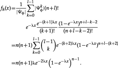
$p_1(t)$ is the probability that a lineage leaves one descendant after time $t$, which is easy to integrate

$$P_1(t)={\displaystyle \int p_1}(t)dt=-\frac{q(t)}{{\mu }^{\prime }},$$ (26)

and gives us the birth–death equivalent of Proposition I:

$$\begin{array}{l}{\displaystyle {\int }_a^b\text{d}}{x}_1{\displaystyle {\int }_a^{x_1}\text{d}}{x}_2\cdots {\displaystyle {\int }_a^{x_{k-1}}\text{d}}{x}_k{\displaystyle \prod _{i=1}^k{p}_1}(x_k)=\\ \frac{1}{k!}{\left(P_1(b)-P_1(a)\right)}^k.\end{array}$$ (27)

For Proposition II we have

$$\begin{array}{l}{\displaystyle {\int }_a^{\infty }\text{d}}{x}_0{\displaystyle {\int }_a^{x_0}\text{d}}{x}_1\cdots {\displaystyle {\int }_a^{x_{k-1}}\text{d}}{x}_k{q}_1(x_0){\displaystyle \prod _{i=0}^k{p}_1}(x_k)=\\ \frac{{{\lambda }^{\prime }}^{-(k+1)}}{(k+2)!}{q}_1{(a)}^{k+2}\end{array}$$ (28)

Which is proved in the Appendix. For the critical case $\lambda =\mu$ we take the limit and use $q_1(t)=\frac{1}{1+{\lambda }^{\prime }t}$ in the formulas above.

Partitioning and Counting

To evaluate the marginal (equations (19) and (10)) we need to establish a valid partitioning and count the number of ranked topologies in each partition. Ideally, the partition would be the smallest possible, that is ${\psi }_1,{\psi }_2\in {\Psi }_{\phi }^k\iff i({\psi }_1)=i({\psi }_2)$. Unfortunately, we were unable to derive a counting formula under this constraint and instead use the clade level partition, a refinement based on the number of lineages per level inside each calibrated clade. Formally, let $r(\psi )=\{r_1,r_2,\cdots ,r_K\}$ where $r_j=(r_{j0},r_{j1},\cdots ,r_{jK})$ and $r_{jk}$ is the number of subclades (not already counted) of the $k$-th calibration point whose rank is smaller than $i_j$. Because $1+{\displaystyle {\sum }_k{r}_{jk}}=i_j$, the equivalence classes induced by $r$ are a refinement of the ones induced by $i(·)$. Furthermore, we can count the number of topologies in each class by using two generic combinatorial principles: First, the number of ways for lineages to coalesce in each level is independent of other levels, so the product of counts of all levels gives the total number of topologies. Second, when $n=n_1+n_2+\cdots +n_j$ lineages enter a level and are reduced to $k=1+k_2+\cdots +k_j$, where lineages can coalesce only within their group ($n_i\to k_i$) and the root of the first group is calibrated ($k_1=1$), the total number of ranked ways is $\left(\begin{array}{c}n-k-1\\ n_1-2,n_2-k_2,\cdots ,n_j-k_j\end{array}\right){\displaystyle {\prod }_{i=1}^j{\text{R}}_{n_i}^{k_i}}$.

${\text{R}}_n^k$ is the number of ranked ways $n$ lineages can coalesce to $k$ (equation (A.1)), and for convenience ${\text{R}}_n={\text{R}}_n^1$.

Figure 2 illustrates the counting procedure on a small example tree.

Figure 2.

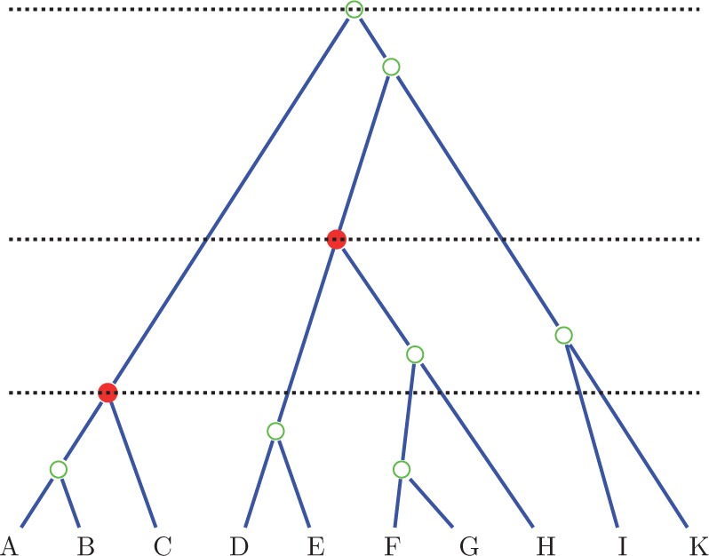
Counting ranked topologies. To count the number of ranked topologies for the tree depicted, we multiply the counts in the three levels. In the lowest level, we have three lineages reducing to one (root of lowest calibration), five lineages reducing to three and two free lineages not reducing. Hence, the total number of topologies is ${\text{R}}_3^1{\text{R}}_5^3{\text{R}}_2^2\left(\begin{array}{c}2+5+2-(1+3+2)\\ 1,2,0\end{array}\right)=3\times (10\times 6)\times 1\times \frac{3!}{1!2!0!}=540$. Note that in the multinomial we use one less lineage (two instead of three) for the calibrated clade, because its position as root is fixed. In the second level, we have three lineages reducing to one, and three free lineages reducing to two, giving ${\text{R}}_3^1{\text{R}}_3^2\left(\begin{array}{c}2+3-(1+2)\\ 1,1\end{array}\right)=3\times 3\times \frac{2!}{1!1!}=18$ and in the last level three lineages to one in three ways. Hence, the total number is $540\times 18\times 3=29,160$.

The use of the clade level partition has an interesting consequence, which relates to the second property of the conditional prior, namely that trees are “Yule-like” (or “birth–death-like”) conditional on the calibrated ages. This means that the density ratio of trees with equal calibrated ages is the same as their density ratio under the uncalibrated tree prior alone (equation (3) in Heled and Drummond (2012)). This condition is relaxed for the restricted conditional prior, where by construction this ratio equality is true only for trees with the same ranked topology. However, because the marginal (equation (17)) depends only on the number of lineages between levels and not on the exact ranked topology, the space in which each tree is “birth–death-like” is in fact larger, containing all trees in the same partition.

Enumerating Ranked Topologies Classes

Here we explain the procedure for explicitly enumerating all the elements of the clade level partition. The enumeration is based upon combining several iterators, one for every calibrated clade, which return the number of lineages in each level of that clade. Those counts are used to compute the marginal as explained in the previous section. The calibrated nodes and the root of the tree, which define the levels, are not included in the counts. We show the working via an example; the interested reader should consult the source code for the very low-level details. The iterator is built from the product of $K+1$ per-clade iterators, one for each calibration and one for the “free” lineages outside any calibrated clade. In fact, each calibrated clade is potentially composed of several calibrated subclades and some free lineages, and the iterator for the clade handles the free lineages and the surviving lineage from the root of each calibrated subclade. Figure 3 gives an example with three calibrated clades, $N$ with $n+2$ lineages, nested inside $M$ with $n+m+3$ lineages, and $L$ with $l+2$ lineages. The uppercase letters are the clade name, and the lowercase letter gives the number of additional lineages.

Figure 3.

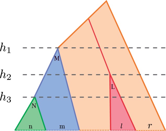
Nested calibrations iterator. The calibrated clades are N (green), M (blue) and L (red), with, respectively, $n+2$, $n+2+m+1$ and $l+2$ taxa. In addition, we have $r$ “free” taxa in orange, which can coalesce between themselves and with the roots of M and L. There are four levels associated with the three calibration nodes, separated by the root ages of the calibrated clades.

In addition there are $r\ge 0$ free lineages, for a total of $n+m+l+5+r$ lineages in the tree. The $m+1$ lineages of $M$ not in $N$ coalesce on the way to the clade root with each other and with the roots of the nested clades, in this case $N$. The $r$ free lineages coalesce with the roots of L and M on the way up, and uncalibrated internal nodes can be in any of the four levels.

Because there are three calibrations there are four levels, separated by the dashed lines, and each per-clade iterator returns four numbers. The iterator of $N$ is trivial, always returning $(n,0,0,0)$, because its root defines the first level. The iterator for $L$ is simple too, because the lineages can coalesce only in the first two levels and there are no free lineages. The iterator returns $(l,0,0,0),(l-1,1,0,0),\dots (0,l,0,0)$.

The iterator for $M$ takes care of $m+1$ free lineages which can coalesce in the first three levels. The iterator returns $(m,0,0,0),(m-1,1,0),(m-1,0,1),(m-2,2,0),(m-2,1,1),(m-2,0,2)\dots ,(0,0,m)$. Basically, the iterator first returns all the cases with $m$ internal nodes in the first level, then all cases with $m-1$ internal nodes in the first level, and so on. The same pattern holds (recursively) for the rest of the levels.

The last iterator takes care of the $r$ free lineages and the surviving lineages of any subclade, here the roots of M and L. In this example this iterator is only necessary if $r>0$, as otherwise there are only two lineages left to deal with. While the internal nodes can be in any of the four levels, there are some restrictions. In general, these restrictions can be quite involved. In this example, the restrictions arise because the enclosing clade (here the root of the tree) has more than one subclade. As a result we always have at least three lineages above $h_2$, and because only two lineages coalesce at the root, the excess has to coalesce in the top two levels. So, the iterator returns $(r-1,0,1,0),(r-1,0,0,1),(r-2,1,1,0)\dots ,(0,0,0,r)$, filling up lower levels first as before, while keeping at least one event in the top two.

Results

Calibrating the Parent of One Clade

Sometimes the calibration information is about the time a particular clade (say a genus, or a species that is divided into subspecies) separated from other lineages in the tree. For a single lineage, the density is given in Heled and Drummond (2012)

$$f_h(x)=2\lambda e^{-2\lambda x}.$$ (29)

Note that the parent age is equal to the (pendant) branch length, and in fact $f_h(x)$ is the distribution of the branch length when conditioning on the number of leaves. Furthermore, because this holds for any branch, we can derive a mean of ${}^1{/}_{2\lambda }$, which reproduces a result discussed by Steel and Mooers (2010).

The result can be generalized to any clade $C$ of size $n$. In that case, let ${\Psi }_{\phi }$ be the set of all genealogies of $n+l$ taxa with a clade on $n$ taxa ($n>1$ and $l>0$) (Fig. 4a).

Figure 4.

Diagrams and notation for three special cases of calibration. a) Calibrating the parent of a clade of size $n$. b) Calibrating a nested clade of size $n$ and the root with a total of $n+m$ taxa. c) Calibrating two nested clades of size $n$ and $n+m$ taxa in a $n+m+l$ taxa tree ($l>0$).

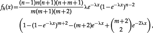
We partition ${\Psi }_{\phi }$ so that ${\Psi }_{\phi }^k$ contains all genealogies containing $k+1$ surviving lineages at $h$, the age of the calibrated parent. By the second counting principle, there are ${\text{R}}_n{\text{R}}_l^i\left(\begin{array}{c}n-2+l-i\\ n-2\end{array}\right)$ ranked ways for lineages to coalesce in the first level, ${\text{R}}_i^{k+1}$ ways for $i$ lineages to reduce to $k+1$ in the second level, and then one of the $k+1$ coalesce with the parent of $C$. Then $k+1$ lineages coalesce to the root, giving

$$\begin{array}{l}|{\Psi }_{\phi }^k|={\displaystyle \sum _{i=k+1}^l{\text{R}}_n}{\text{R}}_l^i\left(\begin{array}{c}n-2+l-i\\ n-2\end{array}\right)(k+1){\text{R}}_i^{k+1}{\text{R}}_{k+1}\\ =(k+1)\left(\begin{array}{c}n-2+l-k\\ n-1\end{array}\right){\text{R}}_n{\text{R}}_l.\end{array}$$ (30)

The total number of ranked trees in ${\Psi }_{\phi }$ is

$$|{\Psi }_{\phi }|={\displaystyle \sum _{k=0}^{l-1}|}{\Psi }_{\phi }^k|=\left(\begin{array}{c}l+n\\ l-1\end{array}\right){\text{R}}_l{\text{R}}_n.$$ (31)

Putting it all together,

(32)

Note that the marginal does not depend the size of the tree, just on the size of the calibrated clade.

Calibrating Two Nested Clades

Here we give the marginal density for two nested clades. When the enclosing clade is the root (Fig. 4b), the marginal is

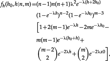(33)

And when the enclosing clade is proper (Fig. 4c), it is

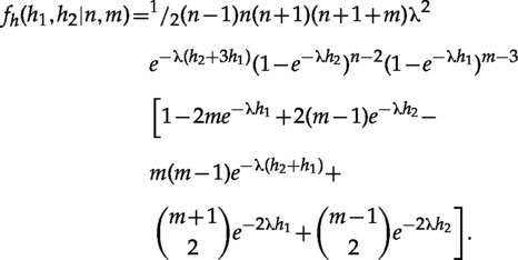(34)

See the Appendix for additional details on the derivation of those formulas.

Placing Additional Monophyly Constraints

It is important to keep in mind that placing additional constraints can invalidate the closed form equations for the marginal. However, it may still be possible to obtain a formula for the full set of constraints. For example, the marginal density for a clade of size $n$ in a $n+m+1$ taxa tree with an outgroup can be obtained by integrating out $h_2$ in equation (34) and is equal to

(35)

which is not equal to the marginal for the same-sized tree where the monophyly on the $n+m$ clade is not enforced.

However, we can derive the marginal in some cases that are not covered by the standard construction (root ages of clades and no extra constraints). For example, take the *BEAST analysis performed as part of the investigation of determining the Pipid root (Bewick et al. 2012). This analysis involves the genera Xenopus, Silurana, Hymenochirus, Pipa, and an outgroup. Five species in total with a four-taxon clade and a calibration on the age of the parent of Pipa. There are $6\times 3$ valid ranked topologies: nine of those have three internal nodes above the calibrated parent, six has two above and one below, and the remaining three has two below and one (the root) above.

The total density for $a$ internal nodes above and $b$ below by equation (17) is

$$f_{a,b}(h)=\lambda e^{-\lambda h}\frac{e^{-\lambda (a+1)h}}{(a+1)!}\frac{{\left(1-e^{-\lambda h}\right)}^b}{b!},$$

and so the marginal is:

$$\begin{array}{l}{f}_h(h)=\frac{5!}{18}\left(9f_{3,0}(h)+6f_{2,1}(h)+3f_{1,2}(h)\right)\\ =\frac{5\lambda e^{-3\lambda h}}{6}\left(e^{-2\lambda h}-4e^{-\lambda h}+6\right).\end{array}$$

AFour-Taxon Tree with One Calibration

Following Heled and Drummond (2012) we consider the following four-taxon tree in which taxa a,B are constrained to be monophyletic and their most recent common ancestor is calibrated with density $f_{AB}$.

There are four ranked topologies in this case, and the 2012 article gives the marginal density for each. Here we wish to contrast the three priors using concrete values: A birth rate of $\lambda {=}^1{/}_2$ and a uniform calibration prior ($f_{AB}=U[4,6]$). Table 1 summarizes the results.

Table 1.

An illustration of the difference between the restricted and full conditional prior using a four-taxa example

		Multiplicative	Conditional	Restricted conditional
Prior “correction term”	((a,b),(c,d)) $T_{CD}<T_{AB}$	–	$3\lambda e^{-3\lambda h_2}$	$12e^{-3\lambda h_2}(1-e^{-\lambda h_2})$
	((a,b),(c,d)) $T_{CD}\ge T_{AB}$
	(((ab),c),d)	–	$3\lambda e^{-3\lambda h_3}$	$4\lambda e^{-4\lambda h_3}$
	(((a,b),d),c)
Marginal Topology probability	((a,b),(c,d))	93%	94.2%	50%
	(((a,b),c),d)	3.5%	2.9%	25%
	(((a,b),d),c)	3.5%	2.9%	25%
Marginal calibration prior		$\frac{3\lambda e^{-3\lambda x}}{e^{-12\lambda }-e^{-18\lambda }}$	$\frac{1}{6-4}$	$\frac{1}{6-4}$

The prior is a pure birth process with a birth rate of $\lambda =\raisebox{1ex}{$1$}\!\left/ \!\raisebox{-1ex}{$2$}\right.$ and a uniform calibration density between four and six is applied to the clade (a,b). The uncorrected (multiplicative) prior is $\frac{1}{6-4}\frac{4!}{4}{\lambda }^3{e}^{-\lambda (2h_1+h_2+h_3)}$, and the table gives the conditional prior “correction terms” for each ranked topology, together with the induced prior probability of each unranked topology and the marginal density for the calibrated clade.

The table lists the “correction term” for each ranked topology, the marginal probability for each unranked topology, and the calibration marginal. As expected, the full and restricted conditional preserve the calibration density, whereas the marginal for the multiplicative prior is equal to the conditional marginal ($3\lambda e^{-3\lambda x}$), bounded between 4 and 6. The marginal topology probability illustrates the difference between the full and restricted priors. The former is similar to the multiplicative prior, with a high probability on the balanced tree. In the space of Yule trees with birth rate ${}^1{/}_2$ and one internal node age between 4 and 6, the other age is far more likely to be smaller than the first. The latter, with equal weight for the two classes, matches the probabilities of the Yule prior without calibration.

Three Calibrations for Bombina

A recent study using 13 complete genomes investigated the phylogenetic relationships of the fire-bellied toads of the genus Bombina (Pabijan et al. 2013). The study contains several types of analysis, and Table 2 of the article lists the sources of the fossil dating used to calibrate the major mitochondrial lineages here. The authors kindly provided us one of the BEAST analyses which uses three nested calibration points, on five taxa, seven taxa, and the root. The results of running the Markov Chain Monte Carlo (MCMC) chain on the multiplicative prior by itself are shown in Figure 5a.

Figure 5.

Three calibrations for Bombina. Three calibration densities for the Bombina analysis, a) under BEAST multiplicative calibration prior and b) under the conditional prior. Each sub-figure shows the density for calibration times (myr), where specified calibration densities are in red, and the induced prior from a BEAST run are in blue. The three fossil calibrations from left to right are for the western Bombina (lognormal distribution with $M=0.0039$ and $S=1.0$, offset by 3.6 myr), the small Bombina (lognormal with $M=0.994$ and $S=1.0$, offset by 13), and for the root (normal distribution with mean 125 and standard deviation of 38).

While the marginal for the two clades deviates only slightly from the specified calibration, the marginal for the root, with mean around 50, is much lower than the normal density calibration $N(\mu =125,\sigma =38)$. The marginals for the analysis using the conditional prior match the calibration densities as expected (Fig. 5b). We also reran the original analysis and a modified version with the conditional prior instead of the multiplicative prior, and the summary trees for the two runs are plotted side by side in Figure 6. Excluding the root, the two analyses produce almost identical divergence times. Becuase the root age dates the divergence of the Discoglossus outgroup, which is incidental in this study, the prior mismatch had no significant effect in this case.

Figure 6.

Summary trees for Bombina analysis. Summary tree from the multiplicative-prior analysis (in black) and the conditional prior (in red). The trees were generated from the posterior using the Common Ancestor method (CAT), which produces the most accurate divergence estimates (Heled and Bouckaert 2013).

Usually the reason for such a close match is hard to see, as the interaction between the prior and the posterior is too complex, but here it seems pretty clear. The analyses used the uncorrelated relaxed clock model (Drummond et al. 2006), and a younger or older root can be “accommodated” by decreasing or increasing the rates on the branches diverging from the root, while maintaining a similar genetic distance. Indeed, the average rate for the longer outgroup branch in the original analysis is 0.044, while the value for the conditional-prior analysis was 0.024. Because the two non-root calibration densities were almost identical, the other divergence times are practically identical.

Two Fossil Calibrations for Sparagnium

Another recent study used two nuclear genes and two chloroplast genes to investigate the systematics, biogeography, and character evolution of Sparganium, a group of aquatic monocots (Sulman et al. 2013). For the divergence dating analysis the authors used a concatenated (supermatrix) approach with two fossil calibrations as detailed in the Calibration points for DNA subsection of their paper. We sample both the multiplicative and conditional calibration priors for this data set. The calibration densities and the induced marginal priors are shown in Figure 7. Under the multiplicative prior, the internal calibration on 27 taxa has a slight preference for older ages whereas the root has a preference for younger ones, compared with the calibration densities. Note that the densities for the two nested clades overlap in the range 90–105 Mya, and so even the conditional prior cannot guarantee the exact marginal for both calibration densities, but the match seems good by visual inspection (Fig. 7).

Figure 7.

Two calibrations for Typhaceae. Two calibration densities for the Sparganium (Typhaceae) analysis under BEAST multiplicative calibration prior a) and the conditional prior b). The specified calibration densities are in black, and the induced prior from a BEAST run is in gray. The crown age of Typhaceae (27 taxa) was constrained to be at least 70 myr (A lognormal with offset 70 and $M=1.5$ and $S=0.5$), and the root constrained with a uniform density between 90 and 105 myr.

We then performed both the original analysis with the multiplicative prior and a modified version with the conditional prior. The summary trees for the two runs are plotted side by side in Figure 8. In this case, the two calibrated (top) nodes have the same estimated divergence time in both analyses, but the non-calibrated nodes in the conditional prior analysis are around 23% younger than their counterparts in the multiplicative prior tree. We can verify that individual divergence times from the two analyses are significantly different by computing the standard error for each estimate, obtained by dividing the standard deviation of the posterior samples by the square root of the effective sample size. For example, the divergence time of the Puya–Brocchinia in the conditional prior analysis is $25.9\pm 0.11$ versus $33.8\pm 0.083$ in the multiplicative prior analysis. Similarly, the Typha root is $5.40\pm 0.036$ versus $7.06\pm 0.037$, and the Sparganium root is $9.75\pm 0.051$ versus $12.62\pm 0.060$.

Figure 8.

Summary trees for Sparganium analysis. Summary Tree from the multiplicative-prior analysis (in black) and the conditional prior (in red). The trees were generated from the posterior using the Common Ancestor method (CAT), which produces the most accurate divergence estimates (Heled and Bouckaert 2013).

Conclusions

We have presented a general approach to specifying a birth–death process tree prior conditional on the heights of a set of calibrated nodes, in the context of the joint inference of topology and divergence times. We have described a few special cases where this prior density has a closed form solution and we have described a general, though computationally intensive, approach to numerical calculation of this conditional density for any number of calibrated nodes. As a result, an arbitrary marginal prior distribution can be precisely specified on the calibrated nodes.

We have also described how the conditional birth–death tree prior naturally induces a nonuniform distribution over ranked topologies. If this effect is unwanted, our approach can be modified to produce a uniform prior on ranked topologies (therefore permitting any arbitrary distribution on ranked tree topologies to be composed with the conditional birth–death prior on divergence times). This modification also renders a computationally efficient algorithm for calculation of the prior density.

To compute the conditional birth–death prior, it is necessary to compute the marginal density of the calibrated node heights averaged over all consistent time-trees. Although we have described some special cases where this marginal prior density of the calibrated nodes can be efficiently computed, it remains to be determined whether other cases have analytical closed-form solutions.

Our implementation is available in BEAST2 (Bouckaert et al. 2014). We regard the full conditional formulation as the correct approach, if one assumes that the birth–death process prior is the appropriate prior for the phylogenetic time-tree under estimation. We therefore recommend the full conditional formulation when computationally feasible (e.g., 2–3 calibrations and/or small numbers of taxa). The restricted formulation effectively removes influence of the birth–death prior on the estimation of the ranked topology and is a good alternative for analyses with larger number of calibrations or taxa for which computational considerations will preclude application of the full conditional. Both of these approaches relieve the practitioner from running their calibrated analysis in the absence of data to determine the resulting marginal distributions (e.g., compare Fig. 5a,b).

We examined and reran two recent BEAST analyses which used a calibrated prior. In both cases the induced prior calibration densities did not match the intended calibrations under the multiplicative prior, but did match as expected with the conditional prior. However, the relevant posterior estimates were not affected in the first case (Bombina), but were significantly different for the second (Sparganium). Hence, while sometimes the estimates are not affected by the change of prior, the two priors can give significantly different results for the same analysis settings and data.

It is clear that development of calibrated tree priors for Bayesian phylogenetic inference remains an area ripe for future development. Obvious next steps would include taking explicit account of the different sources of uncertainty in fossil ages and collection (uncertainty in geological dates, variation in fossil preservation rates, and paleontological discovery effort) and more sophisticated means of dealing with the phylogenetic placement of fossil information (uncertain placement of fossils based on morphological characters of fossils and/or tree prior assumptions). All of these factors are currently subsumed into whatever marginal distribution is specified on the set of calibrated nodes. In the mean time, the work presented here derives new results for multiple-calibration tree priors and in doing so illustrates some of the subtle choices open to the practitioner when calibrating birth–death tree priors.

Funding

J.H. and A.J.D. were supported by a Rutherford Discovery Fellowship from the Royal Society of New Zealand awarded [to A.J.D].

Appendix

Two Nested Clades for the Yule Prior

${\text{R}}_n^k$ is the number of ranked ways $n$ lineages can coalesce to $k$

$$\begin{array}{l}{\text{R}}_n={\displaystyle \prod _{i=2}^n\left(\begin{array}{c}i\\ 2\end{array}\right)}=\frac{n!(n-1)!}{2^{n-1}}\\ {\text{R}}_n^k={\displaystyle \prod _{i=k+1}^n\left(\begin{array}{c}i\\ 2\end{array}\right)}=\frac{{\text{R}}_n}{{\text{R}}_k}=2^{-(n-k)}\frac{n(n-1){!}^2}{k(k-1){!}^2}\end{array}$$ (A.1)

Root and Clade

For the marginal of a clade of $n$ taxa and the root in a $n+m$ taxa tree we partition ${\Psi }_{\phi }$ so that ${\Psi }_{\phi }^k$ contain all topologies with $k+1$ surviving lineages at time $h$ (Fig. 4b). The size of each subset is

$$|{\Psi }_{\phi }^k|=\left(\begin{array}{c}n-2+l-k\\ n-2\end{array}\right){\text{R}}_n{\text{R}}_l^k{\text{R}}_{k+1}$$ (A.2)

and from (Heled and Drummond (2012) appendix C, equation (12)) we have

$$|{\Psi }_{\phi }|=\left(\begin{array}{c}n+l\\ l-1\end{array}\right){\text{R}}_l{\text{R}}_n.$$ (A.3)

Plugging those counts into equation (19) we get

(A.4)

which simplifies to equation (33), because without the $\left(\begin{array}{c}k+1\\ 2\end{array}\right)$, the sum is the binomial expansion of ${(u+v)}^{l-1}$, and with the combinatorial identity

$${\displaystyle \sum _{k=0}^n{(k)}_m}\left(\begin{array}{c}n\\ k\end{array}\right)u^k{v}^{n-k}={(n)}_m{u}^m{(u+v)}^{n-m},$$ (A.5)

we can simplify such sums where the terms are multiplied by any simple polynomial in $k$.

${(x)}_n$ is the Pochhammer symbol, the falling factorial. Here $\left(\begin{array}{c}k+1\\ 2\end{array}\right)=\raisebox{1ex}{$1$}\!\left/ \!\raisebox{-1ex}{$2$}\right.{(k)}_2+{(k)}_1$.

Two nested clades

When the top clade is not the root we need to handle three levels. Let the number of surviving lineages at $h_2$ be $m_1$ and $l_1$, and $l_2$ at $h_1$ (Fig. 4c). We partition ${\Psi }_{\phi }$ according to $m_1$, $l_1$ and $l_2$. that is topologies with the equal values are in the same class.

The number of internal nodes at the three levels is

$$\begin{array}{l}{k}_0=n+m+l-(m_1+l_1+2)\\ k_1=m_1+l_1-(1+l_2)\\ k_2=l_2+1-1.\end{array}$$

The size of each subset is

$$\begin{array}{l}|{\Psi }_{\phi }^{m_1,l_1,l_2}|={\text{R}}_n{\text{R}}_m^{m_1}{\text{R}}_l^{l_1}\frac{k_0!}{(n-2)!(m-m_1)!(l-l_1)!}\\ {\text{R}}_{m_1+1}{\text{R}}_{l_1}^{l_2}\left(\begin{array}{c}{k}_1\\ m_1-1\end{array}\right)\\ {\text{R}}_{l_2+1}.\end{array}$$ (A.6)

Each of the three lines above gives the contribution of one level. The total number of topologies is

$$|{\Psi }_{\phi }|=\left(\begin{array}{c}n+m\\ m-1\end{array}\right){\text{R}}_m{\text{R}}_n\left(\begin{array}{c}n+m+l\\ l-1\end{array}\right){\text{R}}_l.$$ (A.7)

This can be obtained either from summing over all ${\Psi }_{\phi }^{m_1,l_1,l_2}$ terms or more simply by applying Equation (A.3) twice, because the internal clade $N$ does not interact with the free global lineages. Again pluggin those counts into equation (17) we get

$$\begin{array}{l}{f}_{m_1,l_1,l_2}(h_1,h_2)=(n+m+l)!{\lambda }^2{e}^{-\lambda (h_2+h_1)}\frac{e^{-(k_2+1)\lambda h_1}}{(k_2+1)!}\\ \frac{{(1-e^{-\lambda h_2})}^{k_0}}{k_0!}\frac{{(e^{-\lambda h_2}-e^{-\lambda h_1})}^{k_1}}{k_1!}.\end{array}$$ (A.8)

And finally

$$f(h_1,h_2)=|{\Psi }_{\phi }{|}^{-1}{\displaystyle \sum _{m_1=1}^m{\displaystyle \sum _{l_1=1}^l{\displaystyle \sum _{l_2=1}^{l_1}|}}}{\Psi }_{\phi }^{m_1,l_1,l_2}|f_{m_1,l_1,l_2}.$$ (A.9)

The rest is tedious manipulations similar to those in the root and clade case above.

Integral Identity used in Obtaining the Yule Marginal

$${\displaystyle {\int }_h^{\infty }n}\lambda e^{-n\lambda x}{(e^{-\lambda h}-e^{-\lambda x})}^m\text{d}x={\left(\begin{array}{c}m+n\\ n\end{array}\right)}^{-1}{e}^{-(m+n)\lambda h}$$ (A.10)

Proof:

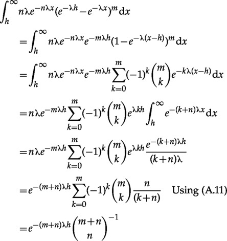The last step used the well-known combinatorial identity (e.g., Sprugnoli (2006), p. 74)

$${\displaystyle \sum _{k=0}^m{(-1)}^k}\left(\begin{array}{c}m\\ k\end{array}\right)\frac{n}{n+k}={\left(\begin{array}{c}m+n\\ n\end{array}\right)}^{-1}.$$ (A.11)

The Birth–Death Prior Marginal

For convenience, let $z=x_{i_1}$ be the age of the last calibration point, and $\hat{c}=c_1-1$, the number of lineages between the root and the last calibration point (excluding the root).

(A.12)

The following solution for the integral can be verified by taking the derivative of the right-hand side

Substituting in equation (A.12) and simplifying gives

(A.13)

The last step uses equation (A.5) for the second sum. Now, after canceling terms and simplifying we are left with

$$P_0(z)=P_0(z,x_1){|}_{x_1=z}^{\infty }=\frac{{{\lambda }^{\prime }}^{-(k+1)}}{(k+2)!}{q}_1{(z)}^{k+2}.$$ (A.14)

References

- Adam J.B., Frédéric J.J.C., Joseph H., Ben J.E. The pipid root. Syst. Biol. 2012;61(6):913–926. doi: 10.1093/sysbio/sys039. [DOI] [PubMed] [Google Scholar]
- Remco R.B., Joseph H., Denise K., Tim V., Chieh-Hsi W., Dong X., Marc A.S., Andrew R., Alexei J.D. Apr. Beast 2: a software platform for bayesian evolutionary analysis. PLoS Comput. Biol. 2014;10:e1003537. doi: 10.1371/journal.pcbi.1003537. doi:10.1371/journal.pcbi.1003537. [DOI] [PMC free article] [PubMed] [Google Scholar]
- Drummond A.J., Rambaut A. Beast: Bayesian evolutionary analysis by sampling trees. BMC Evol. Biol. 2007;7:214. doi: 10.1186/1471-2148-7-214. doi:10.1186/1471-2148-7-214. [DOI] [PMC free article] [PubMed] [Google Scholar]
- Drummond A.J., Ho S.Y.W., Phillips M.J., Rambaut A. Relaxed phylogenetics and dating with confidence. PLoS Biol. 2006;4(5):e88. doi: 10.1371/journal.pbio.0040088. [DOI] [PMC free article] [PubMed] [Google Scholar]
- Felsenstein J. Evolutionary trees from DNA sequences: a maximum likelihood approach. J. Mol. Evol. 1981;17(6):368–376. doi: 10.1007/BF01734359. [DOI] [PubMed] [Google Scholar]
- Alexandra G., David W., Alexei J.D. Recursive algorithms for phylogenetic tree counting. Algorithms for Mol. Biol. 2013;8(1):26. doi: 10.1186/1748-7188-8-26. [DOI] [PMC free article] [PubMed] [Google Scholar]
- Gernhard T. The conditioned reconstructed process. J. Theor. Biol. 2008;253(4):769–778. doi: 10.1016/j.jtbi.2008.04.005. [DOI] [PubMed] [Google Scholar]
- Joseph H., Remco R.B. Looking for trees in the forest: summary tree from posterior samples. BMC Evol. Biol. 2013;13(1):221. doi: 10.1186/1471-2148-13-221. [DOI] [PMC free article] [PubMed] [Google Scholar]
- Joseph H., Alexei J.D. Bayesian inference of species trees from multilocus data. Mol. Biol. Evol. 2010;27(3):570–580. doi: 10.1093/molbev/msp274. [DOI] [PMC free article] [PubMed] [Google Scholar]
- Joseph H., Alexei J.D. Calibrated tree priors for relaxed phylogenetics and divergence time estimation. Syst. Biol. 2012;61(1):138–149. doi: 10.1093/sysbio/syr087. [DOI] [PMC free article] [PubMed] [Google Scholar]
- Sebastian H., Tanja S., Fredrik R., Tom B. Sep. Inferring speciation and extinction rates under different sampling schemes. Mol. Biol. Evol. 2011;28(9):2577–89. doi: 10.1093/molbev/msr095. [DOI] [PubMed] [Google Scholar]
- Huelsenbeck J.P., Ronquist F. MRBAYES: Bayesian inference of phylogenetic trees. Bioinformatics. 2001;17(8):754–755. doi: 10.1093/bioinformatics/17.8.754. [DOI] [PubMed] [Google Scholar]
- David G.K. On the generalized “birth–and-death” process. Ann. Math. Stat. 1948;19(1):1–15. [Google Scholar]
- Kingman J.F.C. The coalescent. Stoch. Proc. Appl. 1982;13(3):235–248. [Google Scholar]
- Hirohisa K., Jeffrey L.T., William J.B. Performance of a divergence time estimation method under a probabilistic model of rate evolution. Mol. Biol. Evol. 2001;18(3):352–361. doi: 10.1093/oxfordjournals.molbev.a003811. [DOI] [PubMed] [Google Scholar]
- Nee S., Holmes E.C., May R.M., Harvey P.H. Apr. Extinction rates can be estimated from molecular phylogenies. Philos. Trans. R. Soc. Lond. B. Biol. Sci. 1994a;344(1307):77–82. doi: 10.1098/rstb.1994.0054. [DOI] [PubMed] [Google Scholar]
- Nee S., May R.M., Harvey P.H. May. The reconstructed evolutionary process. Philos. Trans. R. Soc. Lond. B. Biol. Sci. 1994b;344(1309):305–311. doi: 10.1098/rstb.1994.0068. [DOI] [PubMed] [Google Scholar]
- Pabijan M., Wandycz A., Hofman S., Wecek K., Piwczyński M., Szymura J.M. Complete mitochondrial genomes resolve phylogenetic relationships within bombina (anura: Bombinatoridae) Mol. Phylogenet. Evol. 2013;69(1):63–74. doi: 10.1016/j.ympev.2013.05.007. [DOI] [PubMed] [Google Scholar]
- Rannala B., Yang Z. Sep. Probability distribution of molecular evolutionary trees: a new method of phylogenetic inference. J. Mol. Evol. 1996;43(3):304–11. doi: 10.1007/BF02338839. [DOI] [PubMed] [Google Scholar]
- Rannala B., Ziheng Y. Inferring speciation times under an episodic molecular clock. Syst. Biol. 2007;56(3):453–466. doi: 10.1080/10635150701420643. [DOI] [PubMed] [Google Scholar]
- Renzo S. 2006. An introduction to mathematical methods in combinatorics. Dipartimento di Sistemi e Informatica Viale Morgagni.
- Tanja S. Nov. On incomplete sampling under birth–death models and connections to the sampling-based coalescent. J. Theor. Biol. 2009a;261(1):58–66. doi: 10.1016/j.jtbi.2009.07.018. [DOI] [PubMed] [Google Scholar]
- Tanja S. On incomplete sampling under birth-death models and connections to the sampling-based coalescent. J. Theor. Biol. 2009b;261(1):58–66. doi: 10.1016/j.jtbi.2009.07.018. [DOI] [PubMed] [Google Scholar]
- Mike S., Arne M. The expected length of pendant and interior edges of a yule tree. Appl. Math. Lett. 2010;23:1315–1319. [Google Scholar]
- Joshua D.S., Bryan T.D., Chloe D., Eisuke H., Kenneth J.S. Systematics, biogeography, and character evolution of sparganium (typhaceae): Diversification of a widespread, aquatic lineage. Am. J. Bot. 2013;100(10):2023–2039. doi: 10.3732/ajb.1300048. [DOI] [PubMed] [Google Scholar]
- Jeffrey L.T., Hirohisa K. Divergence time and evolutionary rate estimation with multilocus data. Syst. Biol. 2002;51(5):689–702. doi: 10.1080/10635150290102456. [DOI] [PubMed] [Google Scholar]
- Thorne J.L., Kishino H., Painter I.S. Estimating the rate of evolution of the rate of molecular evolution. Mol. Biol. Evol. 1998;15:1647–1657. doi: 10.1093/oxfordjournals.molbev.a025892. [DOI] [PubMed] [Google Scholar]
- Yang Z., Rannala B. Jul. Bayesian phylogenetic inference using dna sequences: a markov chain monte carlo method. Mol. Biol. Evol. 1997;14(7):717–24. doi: 10.1093/oxfordjournals.molbev.a025811. [DOI] [PubMed] [Google Scholar]
- Yang Z., Rannala B. Bayesian estimation of species divergence times under a molecular clock using multiple fossil calibrations with soft bounds. Mol. Biol. Evol. 2006;23(1):212–226. doi: 10.1093/molbev/msj024. [DOI] [PubMed] [Google Scholar]
- Yule G.U. A mathematical theory of evolution based on the conclusions of dr. j.c. willis. Philos. T. Roy. Soc. B. 1924;213:21–87. [Google Scholar]