Automatic Segmentation and Measurement of Pleural Effusions on CT

Abstract

Pleural effusion is an important biomarker for the diagnosis of many diseases. We develop an automated method to evaluate pleural effusion on CT scans, the measurement of which is prohibitively time consuming when performed manually. The method is based on parietal and visceral pleura extraction, active contour models, region growing, Bezier surface fitting, and deformable surface modeling. Twelve CT scans with three manual segmentations were used to validate the automatic segmentation method. The method was then applied on 91 additional scans for visual assessment. The segmentation method yielded a correlation coefficient of 0.97 and a Dice coefficient of 0.72 ± 0.13 when compared to a professional manual segmentation. The visual assessment estimated 83% cases with negligible or small segmentation errors, 14% with medium errors, and 3% with large errors.

I. Introduction

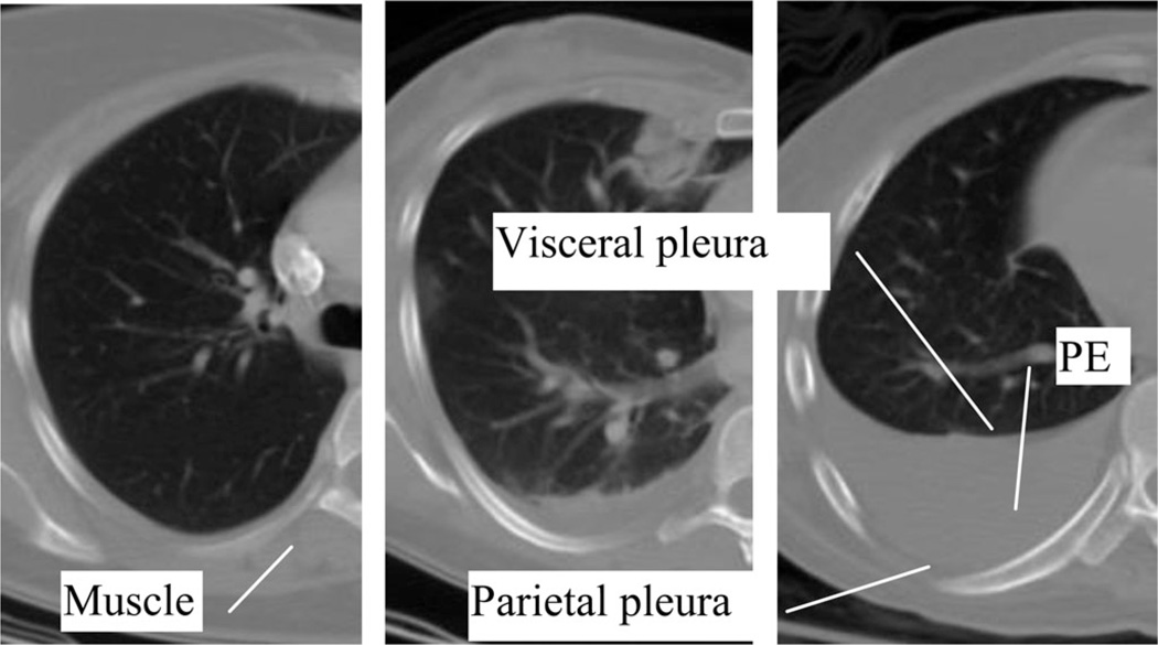
Pleural effusions (PE), buildups of fluid within the pleural cavity, are usually a symptom of a greater illness such as congestive heart failure, pneumonia, or metastatic cancer [1]. They have also been identified as prognostic indicators, for example, for acute pancreatitis [2]. PE can be formed in two ways: transudates where the fluid is pushed into the plural space from elsewhere due to changes in hydrostatic pressure, and exudates where the fluid is created by the pleural surface itself. The pleural cavity is the space between the visceral pleura and the parietal pleura (see Fig. 1). The visceral pleura cover the lungs and the parietal pleura run along the inside of the chest wall. As fluid accumulates in the cavity, it compresses the adjacent lung, undermining lung function. Both the general size and location of the effusion can be diagnostically significant [3] and important to patient care [4].

Fig. 1.

Example CT scans of PE. The shown cases differ in severity (minimal, moderate, and severe from left to right). The pleural space is enclosed by visceral and parietal pleura. Note the similarity between the intensity of muscle and the intensity of PE.

PEs can be detected via a number of noninvasive methods, including chest radiographs, computed tomography (CT) chest studies, and ultrasound (US). CT is increasingly replacing chest radiographs as the dominant method to measure PEs, especially since supine radiographs were found to be less accurate [5]. There have been a variety of attempts to construct a functional US method. Ultrasonic methods offer the best flexibility and portability. One special application of US is in ICU to estimate whether a volume is more or less than 500 mL. When compared to X-ray radiography, many US methods have performed better [6], [7]. When compared to CT, however, the US seems to be less accurate [8], but given the radiation risk of CT and the relative simplicity of the US process, US will be the more viable option in some cases [9]. In most cases, though, the accuracy of CT makes it the better choice.

Though US, radiography, and CT can all be used in manual estimation of effusion size, no fully automated system currently exists that can segment and measure PEs. One method used instead is a bioimpedance technique, but it lacks the accuracy provided by CT [10], and it requires custom hardware. Also, an automatic, CT-based method has been proposed for pneumothorax, but not yet for PEs [11]. Other relevant work with CT scans has focused on specific irregularities such as ascites [12] or indirect methods of estimating volume [13], but these methods require manual segmentation and/or analysis of the radiological images.

PEs can be easily detected and measured in CT scans by radiologists, because the effusion fluid usually has a homogenous signal. However, this process is time consuming, and automatic segmentation faces a major difficulty: the intensity of the fluid from PE is almost identical to that of many surrounding tissues (see Fig. 1). This means that an ordinary region-growing algorithm would be crippled by leaks.

There have been several prior efforts to segment and measure PEs in CT scans. The best segmentation method presented so far came from von Falck et al. [14], but it is not (yet) fully automatic. Though they were able to cut segmentation time by three quarters without sacrificing much segmentation quality, that the software requires physician time at all makes it less than ideal as a routine diagnostic tool (though it may be valuable in special cases). Their algorithm is based on a seven-step process that segments many of the elements of the thorax before isolating the PE [14].

A few more automated methods had also been proposed. Donohue et al. used a slice-by-slice constrained region-based segmentation, and can also segment pulmonary masses [15]. Qian et al. used cubic Hermite curve fitting and bounding box algorithms, using the central column of the image, and a Bessel method estimation of boundary points [16]. Kido and Tsunomori used a conditional region-growing algorithm, constrained by a template built through a global matching process between normal and abnormal lungs and surrounding landmarks [17].

The purpose of this investigation is to develop a fully automated method to segment and measure the volume of PE using routine chest CT images. The program can be run in background to evaluate on clinical CT and return the volume of PE as a valuable biomarker for diagnosis.

II. Materials and Methods

A. CT Scans and Manual Segmentation

This HIPAA-compliant retrospective study was approved by the Institutional Review Board; informed consent was waived. Consecutive routine CT scans from May 2008 to March 2009 in our clinical workflow were used for search. The inclusion criteria are that PE was mentioned in the radiology report. Based on these criteria, 103 scans from 89 patients were selected. Out of those data, 12 scans from 12 patients were manually segmented and used for quantitative evaluation, and the rest were used for qualitative assessment. The average age for the cohort of patients was 54, ranging from 21 to 79, with a standard deviation of 13.9 years. 40 of these patients were women. The CT slices were 512 × 512, with 5-mm slice thickness and in-plane spacing from 0.63 to 0.88 mm. These scans were done with a kVp of 120, on one of three scanners: Siemens Definition, GE LightSpeed Ultra, and Philips Brilliance.

Three sets of manual segmentations were generated for the 12 validation datasets. Two were produced by a research fellow, months apart. The other was produced by a professional image processing technologist. All manual segmentations were made with custom-developed software.

B. Method Overview

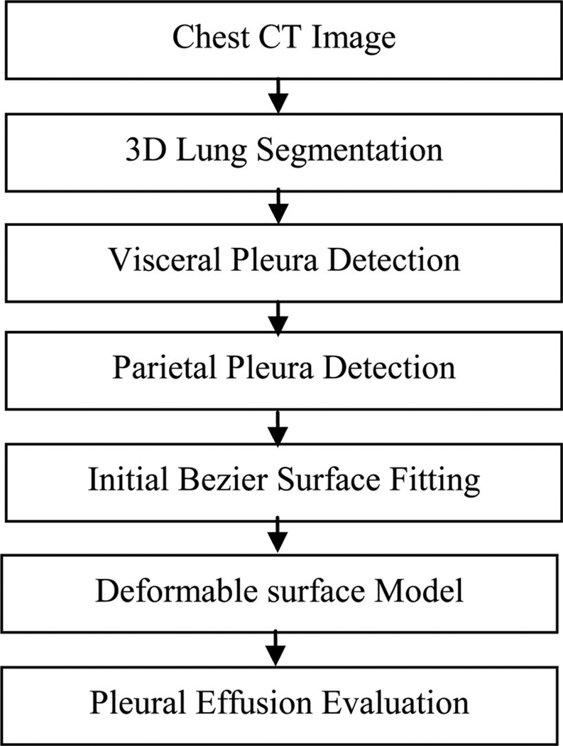
An overview of the method is shown in Fig. 2. Given a CT scan, the program first identifies the border of the lung using a threshold and region growing (see Section II.B2). The pleural space is segmented on each 2-D slice by detecting the visceral and parietal pleura. The visceral pleura are detected using the lung as landmark, and an active contour model (ACM) is used to refine the detection (see Section II.B3). Then, the rib cage is detected and used to fit a B-spline curve to form the parietal pleura (see Section II.B4). The space between visceral and parietal pleura is regarded as the pleural space. After that, a 3-D Bezier surface (see Section II.B5) is fit to all slices to provide an initial value for a deformable surface model (see Section II.B6). The details of these processes are described in the following sections.

Fig. 2.

Schematic of the automatic PE segmentation process.

1) Preprocessing

Preprocessing aims to reduce noise and smooth the image. An anisotropic diffusion filter is used to smooth the intensities of the image without blurring edges [18]. The filter moves pixel intensities toward the average of the surrounding region. Because PEs are usually consistent fluids, the filter makes the signal appropriately consistent without erasing any relevant details. The function itself is given by

$$\frac{\partial }{\partial t}I(\upsilon ,t)=\nabla •(f(\upsilon ,t)\nabla I(\upsilon ,t))$$ (1)

where I(υ, t) represents the image data, υ refers to the pixel coordinate (x, y), t refers to the iteration step. f(υ, t) represents the diffusion function, given by

$$f(\upsilon ,t)=e^{-{(\frac{|\nabla I(\upsilon ,t)|}{K})}^2}$$ (2)

where K is the diffusion constant (default: 3).

2) Lung Segmentation

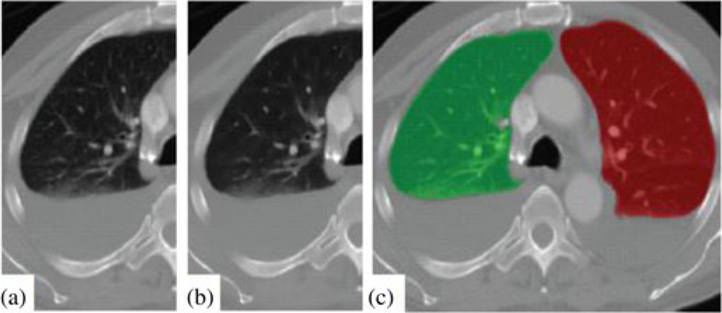
We use a segmentation algorithm previously developed by our group [19]. The lung threshold is determined by analyzing the CT intensity histogram using Otsu’s method [20]. A 3-D region growing method [21] is used to produce a rough segmentation of the lungs. A mathematical morphology technique [21] is then used to fill holes and close gaps. Results of the lung segmentation are shown in Fig. 3(c).

Fig. 3.

Preprocessing and lung segmentation. (a) Original image. (b) After anisotropic diffusion. (c) Lung segmentation mask, green: right lung area, red: left lung area.

3) Visceral Pleura Detection

The pleural space is the space between the visceral and parietal layers of the pleura, which are serous membrane structures. The visceral pleura (inner layer) cover the lungs, and the parietal pleura (outer layer) are attached to the chest wall (see Fig. 1). Most of the pleural fluid is accumulated at the bottom of the pleural space due to gravity. In order to segment the pleural space, the visceral and parietal pleura need to be extracted. The extraction algorithm is applied to the left and right lungs separately.

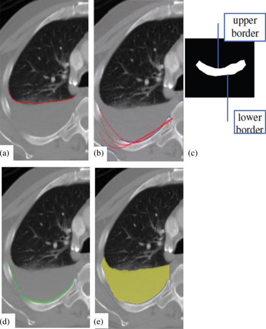
We devise a three-step routine to extract the visceral layer. First, the initial layer is detected at the boundary of the lung; second, a B-spline curve is fitted to the initial layer; and third, an ACM is applied to refine the layer. The initial visceral layer is located at the bottom (posterior) boundary of the lung segmentation. This process can be formulated as

$$\mathrm{V}\mathrm{L}(x)=\underset{y,\mathrm{s}.\mathrm{t}.B(x,y)=1}{\text{arg max}}(B(x,y))B(x,y)=\{\begin{array}{cc}1,\hfill & \text{where}S(x,y)=1,S(x,y+1)=0\hfill \\ 0,\hfill & \text{otherwise}\hfill \end{array}$$ (3)

where B(x,y) is the lung boundary map and S(x,y) is the lung segmentation mask. (x,VL(x)) is the initial value for the visceral layer, which is shown in Fig. 4(a). The initial value is then fitted into a smooth B-spline curve [22], written as

$$N_{i,d}(t)=\frac{t-t_i}{t_{i+d}-t_i}{N}_{i,d-1}(t)+\frac{t_{i+d+1}-t}{t_{i+d+1}-t_{i+1}}{N}_{i+1,d-1}(t)C(t)=\sum _{i=0}^n{P}_i{N}_{i,d}(t)$$ (4)

where C(t) is the fitted curve, T ={t₀, t_n} are evenly distributed internal knots, N(t) are the basis functions, d is the degree of the curve (default value is five), and P_i = (x,VL(x)) are the control points (100 control points are uniformly sampled), the initial estimate of the visceral layer. Once the constants in this equation are determined and a function is fitted, it is used as an initial value in an ACM [23] to further refine the visceral layer. The force operating on the ACM is

$$F=w_{\text{in}}{F}_{\text{internal}}+w_{im}{F}_{\text{image}}$$ (5)

where F_internal is the spline force of the contour, F_image is the image force, and w terms are weights. The internal force is defined as

$$F_{\text{internal}}=\frac{1}{2}{\int }_0^1(\alpha (s)|c\prime (s){|}^2+\beta (s)|c\prime (s){|}^2)ds$$ (6)

where α and β control the elasticity and rigidity of ACM(default 0.5 and 1), c(s) is the curve representing the contour, and c′ and c″ are the first and second derivatives of c(s), respectively. This force tends to straighten the curve. The image force pushes the curve toward edges, specifically, the border between the lung and the PE (or ribcage). The image force is given by

$$F_{\text{image}}=\stackrel{\rightharpoonup }{g}(|I\prime (x)|)$$ (7)

where g⃑ is the gradient operator and I′(x) is the first-order derivative of image I.

Fig. 4.

Visceral and parietal pleura extraction. (a) Curve identified as visceral pleura. (b) Iterative refinement of the parietal pleura curve. (c) Slab model of the ribcage. (d) Curve identified as parietal pleura. (e) Resulting 2-D PE segmentation.

4) Parietal Pleura Detection

The parietal layer is detected after the visceral layer is identified. We use a similar three-step routine for the parietal pleura extraction. First, landmark points on the inner rib cage are detected; second, a Bernstein polynomial is fitted to the landmarks; and third, an ACM is applied to refine the layer.

The algorithm searches below the visceral layer (in the posterior direction) and identifies points of high intensity. These points are assumed to be part of the ribcage, and are then used to model the ribcage as an elongated slab [see Fig. 4(c)]. The model maximizes the difference in intensity gradient between its anterior and posterior borders, such that those borders line up with the edges of the bone. The searching process can be written as

$$VU(x)=\underset{y^u,y^l}{\text{arg max}}(g(I(x,y^u))-g(I(x,y^l)))\text{where}I(x,y^u)>\text{th},I(x,y^l)>\text{th},t_{\text{min}}<y^u-y^l<t_{\text{max}}$$ (8)

where I(x,y) is the image intensity, g(I(x,y)) is the image gradient, th is the bone intensity threshold (default:300HU), t_min and t_max is the range of rib width (default values: 5 and 20 mm). The upper border points (x, y^u) are collected as landmarks [see Fig. 4(b)].

A Bernstein polynomial is then fitted to the points of the anterior border of the model, and an ACM is used to refine the layer. The Bernstein polynomial is written as

$$y=P(a_0\dots ,a_5;x)=\sum _{k=0}^5{a}_k\left(\begin{array}{c}\hfill 5\hfill \\ \hfill k\hfill \end{array}\right){(1-x)}^k{x}^{5-k}.$$ (9)

The fitting operation finds the constant that minimizes the least-square measure, Σ [y_i−P(a₀ .…,a₅;x_i]², where (x_i, y_i) are landmark points. This fitting is run in three iterations, between which outliers are eliminated. At each iteration, the curve is used as the initial for the ACMs to generate the estimate of the parietal layer [see Fig. 4(b) and (d)].

5) Initial PE Surface Fitting

The endpoints of the two curves (visceral and parietal layers) thus produced are connected with straight lines to form a closed shape, and all pixels that fall inside are defined as PE using a scanline algorithm [see Fig. 4(e)] [24].

Once the pleural space is segmented on each 2-D slice, the edges of the entire PE segmentation are evenly sampled (200 sample points are used). These are used as control points to generate a Bezier surface. Bezier surface is defined by

$$p(u,\upsilon )=\sum _{i=0}^n\sum _{j=0}^m{Z}_i^n(u)Z_j^m(\upsilon )k_{i,j}$$ (10)

where p(u, υ) is a point on the surface, (n,m) is the degree of the surface, which varies with the number of control points, Z is the Bezier surface function, and k_i,j is the set of control points. The surface is, by definition, stretched among the control points so as to render the single, smooth surface they approximate [25]. This process smoothes the segmentation and corrects certain errors in the initial segmentation.

6) Three-Dimensional Deformable Modeling of Pleural Space

A deformable surface model is then applied to refine the boundary of the PE using the Bezier surface as initial. The model is driven by both internal spline forces and external image forces, which can be written as

$$F(\upsilon )=\alpha \nabla s(\upsilon )-\beta \nabla (\nabla s(\upsilon ))+\gamma \nabla (G_{\sigma }(|\nabla G_{\sigma }(I(\upsilon )){|}^2))$$ (11)

where s is the surface model, υ is a vertex on the model, and ∇ is the partial derivatives. G_σ is the Gaussian operator. |∇G_σ (I(υ))/² computes the gradient magnitude, which represents an edge map. The location of a vertex υ on the model is updated at each iteration

$${\upsilon }^{(t)}={\upsilon }^{(t-1)}+\tau F({\upsilon }^{(t-1)})$$ (12)

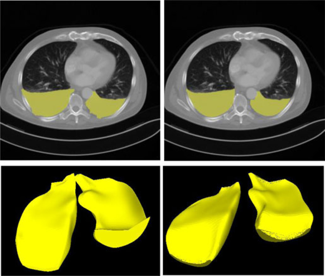
where t is the evolution time, τ is the step size, and F is the deformation force. Fig. 5 shows the result of the deformable surface model. The pixels contained by this surface are counted and converted to the total volume in cubic centimeters.

Fig. 5.

Three-dimensional deformable surface model. (Top left) Two-dimensional segmentation result before the deformable surface model. (Top right) Two-dimensional segmentation result after the deformable surface model. (Bottom) Segmented PE surface [before (left) and after (right) deformable surface modeling].

III. Results

We conducted validation experiments on a small cohort of patients using manual segmentations, and ran the program on a large cohort of clinical data for qualitative evaluation.

A. Validation Experiments

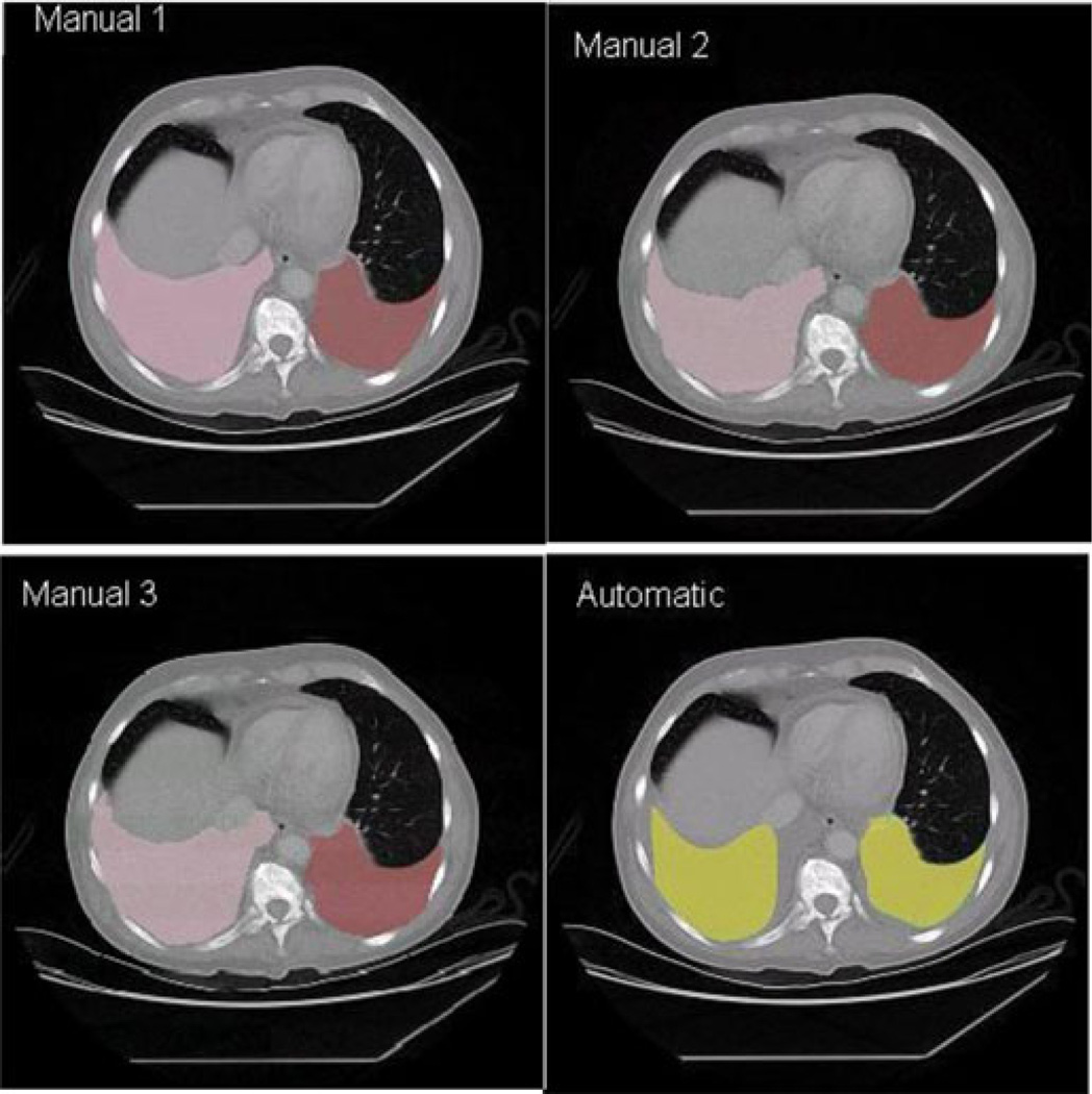
The validation of our method was conducted on 12 CT studies with three sets of manual segmentations. Six comparisons were made: three for the automatic against the manual segmentations and three among the manual segmentations to estimate interoperator variability. Manual segmentations 1 and 2 were performed by the same fellow, months apart. Segmentation 3 was performed by a professional image processing technologist. An example of a slice in each of the segmentation is shown in Fig. 6. For each comparison, the total volume of the manual segmentation, total volume from the automatic segmentation, total overlap volume, and Dice coefficient were calculated.

Fig. 6.

Comparison of segmentations. Manuals 1 and 2 were performed by the same fellow, months apart. Manual 3 was performed by a professional CT technologist. The automatic, manual left lung, and manual right lung segmentations are shown in yellow, brown, and pink, respectively.

Based on these data, percent total error, percent overlap, false positive rate (FPR), and Dice coefficient were calculated for each comparison according to the following equations, where OLV is the overlap volume, TMV is the total manual volume, and TAV is the total automatic volume (the same calculation was used to compare two manual volumes, as well)

$$\text{Dice}=2*\mathrm{O}\mathrm{L}\mathrm{V}/(\mathrm{T}\mathrm{M}\mathrm{V}+\mathrm{T}\mathrm{A}\mathrm{V})\text{Overlap}=\mathrm{O}\mathrm{L}\mathrm{V}/\mathrm{T}\mathrm{M}\mathrm{V}\mathrm{F}\mathrm{P}\mathrm{R}=(\mathrm{T}\mathrm{A}\mathrm{V}-\mathrm{O}\mathrm{L}\mathrm{V})/\mathrm{T}\mathrm{A}\mathrm{V}.$$ (13)

Averages and standard deviation of these values for all 12 validation cases were calculated for each type of comparison (see Table I). Performance differed significantly from comparison to comparison, but the results from the automatic segmentations are comparable to those from the comparisons among manual segmentations.

TABLE I.

Dice Coefficients, TPs, and FPs

Dice\TP|FP	Auto	Manual 1	Manual 2	Manual 3
New Auto	x	0.72|0.32	0.74|0.34	0.68|0.23
Manual 1	0.69±0.19	x	0.80|0.13	0.71|0.16
Manual 2	0.69±0.17	0.83±0.10	X	0.69|0.13
Manual 3	0.72±0.13	0.76±0.16	0.70±0.13	x
Average Dice	0.70±0.16	0.71±0.13	0.70±0.13	0.67±0.2
Manual vs Manual average:			0.73

Note: Dice coefficients and their standard deviations are shown in the bottom left, true positive (TP) and false positive (FP) rates are shown in the upper right.

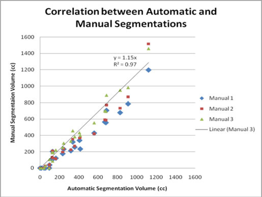
The Dice values are roughly similar, all around 0.7, except for the intrapersonal comparison, which is 0.83 ± 0.10. The Dice coefficient for the comparison between Manuals 1 and 2 was 0.11 higher than for any comparison with the automatic segmentation, and the comparison had a high overlap rating, as well (0.80) (see Table I). The correlation between the automatic and manual estimates of PE volume is 0.97 (see Fig. 7).

Fig. 7.

Correlations between automatic and manual segmentation volumes.

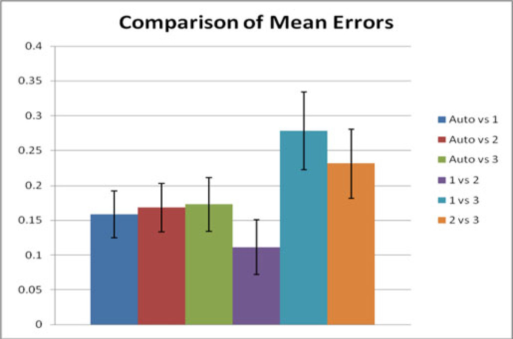
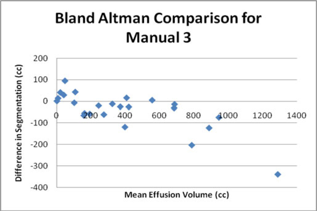
Other potentially useful statistics are the average percent error in PE volume. The intraobserver comparison of manual segmentations had the lowest average error of 11%. The comparisons between the manual segmentations performed by a fellow and the professional technologist had average errors of 23% and 28%. The comparisons between the manual segmentations 1, 2, and 3 and the automatic segmentation had average errors of 16%, 17%, and 17%, respectively (see Fig. 8). The error of the comparisons with the automatic segmentations was significantly lower (p < 0.05) than the error of one of the interpersonal comparisons (Manual 1 versus Manual 3). A Bland–Altman plot, comparing the professional technologist’s manual segmentation to the automatic segmentation, is given in Fig. 9.

Fig. 8.

Comparison of average errors. The average error (%) was calculated by dividing the difference between two segmentations by the mean total volume. The means and errors of these values from the 12-patient validation set are displayed.

Fig. 9.

Bland–Altman plot comparing the automatic segmentation to manual segmentation 3.

B. Qualitative Evaluation in a Large Cohort

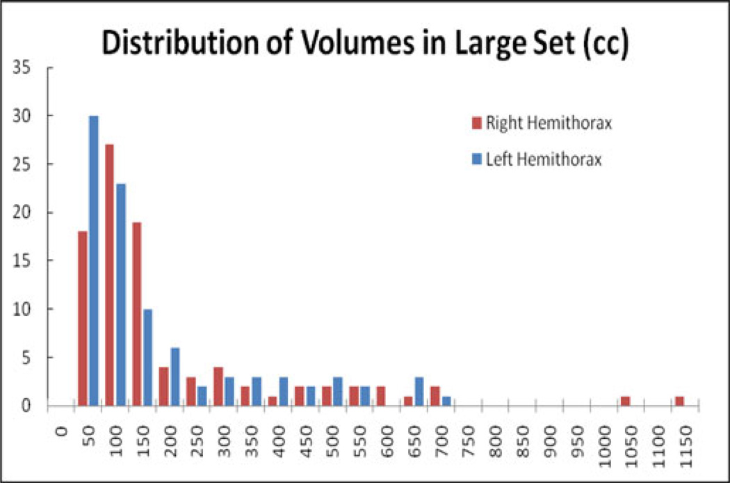
The large set of scans (91 scans, 77 patients) was used to gain a qualitative understanding of the program’s function. The distribution of PE volume per lung by the automatic measurement is shown in Fig. 10.

Fig. 10.

Distribution of PE volumes. The median was 90 cc, Q1 was 49 cc, and Q3 was 192 cc. For the left lung, the median was 103 cc, Q1 was 55 cc, and Q3 was 222 cc. For the right lung, the median was 85 cc, Q1 was 42 cc, and Q3 was 192 cc.

The majority of PE segmentations are smaller than 200 cc, but there is a fat tail that ends with three effusions that were measured as just under 700 cc. There are also two outliers above 1000 cc. A user visually examined the computer segmentation and estimated the segmentation error in four categories (Negligible: <3%; small: <10%; medium <20%; large:> = 20%). Based on the rules, 20 datasets (22%) were estimated as negligible; 55 datasets (61%) as small, 13 datasets as medium (14%); and three cases (3%) as large.

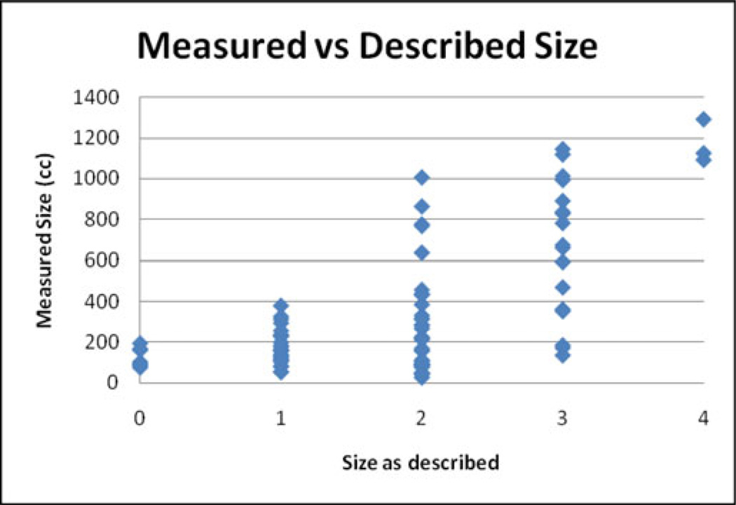
Based on the reports from the radiologists who performed the clinical analyses, of the 88 samples (those reports that did not use these terms were excluded), 28 had “minimal,” “very small,” or “tiny” PEs, 34 had small PEs, 15 had moderate PEs, 4 had large PEs, and 7 had no PEs. Fig. 11 shows the distribution of the automatic estimates of size compared to radiologists’ estimates—refer to Fig. 10 for the distribution of the sizes themselves. The radiologists made these estimates as part of routine examinations, so they may not have been taken seriously and certainly were not standardized across individuals, but they do indicate at a basic level the distribution of effusion sizes in the sample. The automatic measurement missed some loculated PEs, which contribute to some of the discrepancy.

Fig. 11.

Comparison of measured volume with radiologist estimates: 0 means that the radiologist described the effusion as resolved or nonexistent; 1 means they described it as “tiny,” “very small,” or “minimal”; 2, 3, and 4 mean they described it as “small,” “moderate,” and “large,” respectively.

IV. Discussion and Conclusion

Judging by the data in Table I, our automatic segmentation is comparable to the manual segmentations that are currently available. The performance appears not to be on par with the best manual-to-manual comparison. However, given the high correlation coefficient achieved, the automatic segmentation may give strong estimations of the total volume, especially in large PEs.

The program works best with PEs that have a specific shape: they start on the posterior side of the lung and extend in the inferior direction without moving far in the anterior direction below the bottom of the lung. The method cannot be used to measure loculated effusions, for example, since the initial segmentation assumes that the effusion is posterior to the lung.

Our method is quite sophisticated and incorporates several advanced image processing. We did try other classic segmentation techniques such as thresholding, region growing, and fuzzy connectness. However, they failed in most cases. A few specific models were chosen in our method due to their effectiveness and availability to us. Bernstein polynomial curve was used to model the parietal layer. The main reason is to eliminate outliers caused by shoulder bones and leakage since it is a global fitting and stable. Bezier surface was used for the 3-D surface modeling of PE since it is numerically stable, robust to the control point selection, and efficient to compute. We used ACM to further refine the segmentation of the visceral layer due to its effectiveness and availability to us. Li and Acton [26] recently added a vector field convolution (VFC) force to ACM to improve its robustness and capture range. We intend to try out VFC in our future work.

We have made a major step toward having a clinically useful program. This program could be used as part of a chest CT routine to produce data that may yield diagnostically significant trends in PE size. Since the program is fully automated and very efficient (less than 1min), it is convenient to incorporate it in the clinical workflow. It can be run in the background right after the CT is acquired and the PE volume will be ready as a biomarker when the radiologists are reading the case.

References

- 1.Light RW. Pleural effusion. New Engl. J. Med. 2002;346:1971–1977. doi: 10.1056/NEJMcp010731. [DOI] [PubMed] [Google Scholar]
- 2.Lankisch P, Dröge M, Becher R. Pleural effusions: A new negative prognostic parameter for acute pancreatitis. Amer. J. Gastroenterol. 1994;89:1849–1851. [PubMed] [Google Scholar]
- 3.Porcel J, Vives M. Etiology and pleural fluid characteristics of large and massive effusions. Chest. 2003;124:978–983. doi: 10.1378/chest.124.3.978. [DOI] [PubMed] [Google Scholar]
- 4.Medford A, Maskell N. Pleural effusion. Postgrad. Med. J. 2005;81:702–710. doi: 10.1136/pgmj.2005.035352. [DOI] [PMC free article] [PubMed] [Google Scholar]
- 5.Ruskin JA, Gurney JW, Thorsen MK, Goodman LR. Detection of pleural effusions on supine chest radiographs. Amer. J. Roentgenol. 1987;148:681–683. doi: 10.2214/ajr.148.4.681. [DOI] [PubMed] [Google Scholar]
- 6.Usta E, Mustafi M, Ziemer G. Ultrasound estimation of volume of postoperative pleural effusion in cardiac surgery patients. Interact. Cardiovasc. Thoracic Surg. 2009;10:204–207. doi: 10.1510/icvts.2009.222273. [DOI] [PubMed] [Google Scholar]
- 7.Vignon P, Chastagner C, Berkane V, Chardac E, Francois B, Normand S, Bonnivard M, Clavel M, Pichon N, Preux PM, Maubon A, Gastinne H. Quantitative assessment of pleural effusion in critically ill patients by means of ultrasonography. Crit. Care Med. 2005;33:1757–1763. doi: 10.1097/01.ccm.0000171532.02639.08. [DOI] [PubMed] [Google Scholar]
- 8.Roch A, Bojan M, Michelet P, Romain F, Bregeon F, Papazian L, Auffray J-P. Usefulness of ultrasonography in predicting pleural effusions >500 ml in patients receiving mechanical ventilation. Chest. 2005;127:224–232. doi: 10.1378/chest.127.1.224. [DOI] [PubMed] [Google Scholar]
- 9.Balik M, Plasil P, Waldouf P, Pazout J, Fric M, Otahal M, Pachl J. Ultrasound estimation of volume of pleural fluid in mechanically ventilated patients. Intensive Care Med. 2006;32:318–321. doi: 10.1007/s00134-005-0024-2. [DOI] [PubMed] [Google Scholar]
- 10.Arad M, Zlochiver S, Davidson T, Shoenfeld Y, Adunsky A, Abboud S. The detection of pleural effusion using a parametric fit technique. Physiol. Meas. 2009;30:421–428. doi: 10.1088/0967-3334/30/4/006. [DOI] [PubMed] [Google Scholar]
- 11.Cai W, Tabbara M, Takata N, Yoshida H, Harris GJ, Novelline RA, de Moya M. MDCT for automated detection and measurement of pneumothoraces in trauma patients. Amer. J. Roentgenol. 2009;192:830–836. doi: 10.2214/AJR.08.1339. [DOI] [PubMed] [Google Scholar]
- 12.Halvorsen R, Fedyshin PJ, Korobkin M, Foster WL, Jr, Thompson WM. Ascites or pleural effusion? CT differentiation: Four useful criteria. RadioGraphics. 1986;6:135–149. doi: 10.1148/radiographics.6.1.3685482. [DOI] [PubMed] [Google Scholar]
- 13.Mergo PJ, Helmberger T, Didovic J, Cernigliaro J, Ros PR, Staab EV. New formula for quantification of pleural effusions from computed tomography. J. Thorac. Imag. 1999;14:122–125. doi: 10.1097/00005382-199904000-00011. [DOI] [PubMed] [Google Scholar]
- 14.von Falck C, Meier S, Jordens S, King B, Galanski M, Shin HO. Semiautomated segmentation of pleural effusions in MDCT datasets. Acad. Radiol. 2010;17:841–848. doi: 10.1016/j.acra.2010.02.011. [DOI] [PubMed] [Google Scholar]
- 15.Donohue R, Shearer A, Bruzzi J. Constrained region-based segmentation of pleural effusion in thin-slice CT. Proc. IEEE 13th Int. Mach. Vis. Image Process. Conf. 2009:24–29. [Google Scholar]
- 16.Qian Y, Zhang C, Yang X. New method for quantification of pleural effusions from CT imaging. Proc. ISECS Int. Colloq. Comput. Commun. Control Manage. 2008:768–773. [Google Scholar]
- 17.Kido S, Tsunomori A. Automated extractions of pleural effusion in three dimensional thoracic CT images. SPIE Med. Imaging. 2009;7260:72600D1–72600D8. [Google Scholar]
- 18.Weickert J. Anisotropic Diffusion in Image Processing. Stuttgart, Germany: B. G. Teubner; 1998. [Google Scholar]
- 19.Yao J, Dwyer A, Summers RM, Mollura DJ. Computer-aided diagnosis of pulmonary infections using texture analysis and support vector machine classification. Acad. Radiol. 2011;18(3):306–314. doi: 10.1016/j.acra.2010.11.013. [DOI] [PMC free article] [PubMed] [Google Scholar]
- 20.Otsu N. A threshold selection method from gray-level histograms. IEEE Trans. Syst., Man., Cybern. 1979 Jan;9(1):62–66. [Google Scholar]
- 21.Rogowska J. Overview and fundamentals of medical image segmentation. In: Bankman IN, editor. Handbook of Medical Imaging, Processing and Analysis. New York, NY, USA: Academic; 2000. pp. 69–85. [Google Scholar]
- 22.Weisstein EW. CRC Concise Encyclopedia of Mathematics. 2nd ed. London, U.K: Chapman & Hall; 1999. [Google Scholar]
- 23.Kass M, Witkin A, Terzopoulos D. Snakes:Active contour models. Int. J. Comput. Vis. 1988;1:321–331. [Google Scholar]
- 24.Wolberg G. Digital Image Warping. Washington, DC, USA: IEEE Computer Society Press; 1990. [Google Scholar]
- 25.Farin G. Curves and Surfaces for Computer Aided Geometric Design: A Practical Guide. 2nd ed. New York, NY, USA: Academic; 1990. [Google Scholar]
- 26.Li B, Acton ST. Active contour external force using vector field convolution for image segmentation. IEEE Trans. Image Process. 2007 Aug;16(8):2096–2106. doi: 10.1109/tip.2007.899601. [DOI] [PubMed] [Google Scholar]