SCALABLE FUSED LASSO SVM FOR CONNECTOME-BASED DISEASE PREDICTION

Abstract

There is substantial interest in developing machine-based methods that reliably distinguish patients from healthy controls using high dimensional correlation maps known as functional connectomes (FC's) generated from resting state fMRI. To address the dimensionality of FC's, the current body of work relies on feature selection techniques that are blind to the spatial structure of the data. In this paper, we propose to use the fused Lasso regularized support vector machine to explicitly account for the 6-D structure of the FC (defined by pairs of points in 3-D brain space). In order to solve the resulting nonsmooth and large-scale optimization problem, we introduce a novel and scalable algorithm based on the alternating direction method. Experiments on real resting state scans show that our approach can recover results that are more neuroscientifically informative than previous methods.

1. INTRODUCTION

There is substantial interest in establishing neuroimaging-based biomarkers that reliably distinguish individuals with psychiatric disorders from healthy individuals [1]. Functional connectomes (FC's) generated from resting state fMRI has emerged as a mainstream approach, offering robust ability to characterize the network architecture of the brain [2, 3]. FC's are typically generated by parcellating the brain into hundreds of distinct regions, and computing cross-correlation matrices [4]. However, even with a relatively coarse parcellation with several hundred regions of interest (ROI), the resulting FC contains nearly a hundred thousand connections or more, presenting critical statistical and computational challenges.

In the high dimensional setup, sparsity is a natural assumption that arises in many applications [5, 6]. Indeed, most existing methods address the dimensionality of FC's by applying some form of a priori feature selection (e.g., t-test) before invoking some “off-the-shelf” classifier (e.g., nearest-neighbor, support vector machine (SVM), LDA) [3]. Sparsity promoting regularizers such as Lasso [7] and Elastic-net [8] may also be considered. However, all these methods above have a major shortcoming: outside of sparsity, the structure of the data is not taken into account.

Recently, there has been strong interest in the machine learning community in designing a convex regularizer that promotes structured sparsity [9, 10]. Indeed, spatially informed regularizers have been applied successfully for decoding in task-based fMRI, where the goal is to localize in 3-D space the brain regions that become active under an external stimulus [11, 12]. FC's exhibit rich spatial structure, as each connection comes from a pair of localized regions in 3-D space, giving each connection a localization in 6-D space (referred to as “connectome space” hereafter). However, no framework currently deployed exploits this spatial structure.

Based on these considerations, the main contribution of this paper is two-fold: (1) to account for the 6-D spatial structure of FC's, we propose to use the fused Lasso regularized SVM (FL-SVM) [13], and (2) we introduce a novel scalable algorithm based on the alternating direction method [14] for solving the nonsmooth, large-scale optimization problem that results from FL-SVM. To the best of our knowledge, this is the first application of structured sparse methods in the context of disease prediction using FC's. Experiments on real resting state scans demonstrate that our method can identify predictive features that are spatially contiguous in the connectome space, offering an additional layer of interpretability that could provide new insights about various disease processes.

2. METHODS

FMRI data consist of a time series of three dimensional volumes imaging the brain, where each 3-D volume encompasses around 10, 000~100, 000 voxels. The univariate time series at each voxel represents a blood oxygen level dependent (BOLD) signal, an indirect measure of neuronal activities in the brain. Traditional experiments in the early years of fMRI research involved task-based studies, but after it was discovered that the brain is functionally connected at rest, resting state fMRI became a dominant tool for studying the network architecture of the brain. As such, we used the time series from resting state fMRI to generate FC's, which are correlation maps that describe brain connectivity.

More precisely, resting state FC's were produced as follows. First, 347 spherical nodes are placed throughout the entire brain over a regularly-spaced grid with a spacing of 18 × 18 × 18 mm; each of these nodes represent an ROI with a radius of 7.5 mm, which encompasses 30 voxels (the voxel size is 3 × 3 × 3 mm). Next, for each of these nodes, a single representative time series is assigned by spatially averaging the BOLD signals falling within the ROI. Then, a cross-correlation matrix is generated by computing Pearson's correlation coefficient between these representative time series. Finally, a vector x of length $\left(\begin{array}{c}\hfill 347\hfill \\ \hfill 2\hfill \end{array}\right)=60,031$ is obtained by extracting the lower-triangular part of the cross-correlation matrix; this vector is the FC that serves as the vector prediction.

Fused Lasso Support Vector Machine (FL-SVM)

Our goal is to learn a linear decision function sign (〈x, w〉) given a set of training input/output pairs ${\left\{({\mathit{x}}_i,y_i)\right\}}_{i=1}^n$, where ${\mathit{x}}_i\in {\mathbb{R}}^p$ represents the FC's, and y_i ∈ {±}1 indicates the diagnostic status of subject i. The SVM aims to learn the weight vector ${\mathbb{R}}^p$ by minimizing the following problem:

$$\underset{\mathit{w}\in {\mathbb{R}}^p}{\arg \min }\sum _{i=1}^n\ell \left(y_i\langle \mathit{w},{\mathit{x}}_i\rangle \right)+\mathcal{R}\left(\mathit{w}\right),$$ (1)

where $\ell \left(y_i\langle \mathit{w},{\mathit{x}}_i\rangle \right)={(1-y_i\langle \mathit{w},{\mathit{x}}_i\rangle )}_{+}$ is the hinge loss and $\mathcal{R}:{\mathbb{R}}^p\to {\mathbb{R}}_{+}$ is the regularizer. For compactness, we introduce the notation Y := diag{y₁, , y_n} and design matrix $\mathit{X}\in {\mathbb{R}}^{n\times p}$ created from stacking the feature vectors ${\left\{x_i\right\}}_{i=1}^n$ as rows. This allow us to express the loss term in (1) succinctly by defining a functional $\mathcal{L}:{\mathbb{R}}^n\to {\mathbb{R}}_{+}$ which aggregates the total loss $\mathcal{L}\left(\mathit{Y}\mathit{X}\mathit{w}\right)≔{\sum }_{i=1}^n\ell \left(y_i\langle \mathit{w},{\mathit{x}}_i\rangle \right)$.

In our application, we seek a model that is not only accurate but also interpretable. The standard SVM [15] uses the ${\ell }_2$-norm regularizer $\mathcal{R}\left(\mathit{w}\right)=\lambda {\Vert \mathit{w}\Vert }_2^2$, which is problematic for interpretation since it yields a non-sparse and dense solution. Sparsity promoting regularizers such as the Lasso $\mathcal{R}\left(\mathit{w}\right)=\lambda {\Vert \mathit{w}\Vert }_1$ and Elastic-net $\mathcal{R}\left(\mathit{w}\right)=\lambda {\Vert \mathit{w}\Vert }_1+\frac{\gamma }{2}{\Vert \mathit{w}\Vert }_2^2$ can be used for automatic feature selection [7, 8], but these approaches do not account for the spatial structure of the FC's. To address this issue, we employ the fused Lasso [13].

Fused Lasso was originally designed to encode correlations among successive variables in 1-D, but can be extended to other situations where there is a natural ordering among the feature coordinates. This is the case with our 6-D FC's due to the grid pattern in the nodes, and the FL-SVM problem reads:

$$\underset{\mathit{w}\in {\mathbb{R}}^p}{\arg \min }\mathcal{L}\left(\mathit{Y}\mathit{X}\mathit{w}\right)+\lambda {\Vert \mathit{w}\Vert }_1+\gamma {\Vert \mathit{C}\mathit{w}\Vert }_1,$$ (2)

where $\mathit{C}\in {\mathbb{R}}^{e\times p}$ denotes the 6-D differencing matrix, and ${\Vert \mathit{C}\mathit{w}\Vert }_1={\sum }_{j=1}^p{\sum }_{k\in {\mathcal{N}}_j}\mid w_j-w_k\mid$ is a spatial penalty that accounts for the 6-D structure in the connectome by penalizing deviations among the nearest-neighbor edge set ${\mathcal{N}}_j$. Note that e indicates the total number of unordered pairs of adjacent coordinates. To gain a better understanding of ${\mathcal{N}}_j$, let us denote (x, y, z) and (x′, y′, z′) the pair of 3-D points in the brain that define the 6-D connectome coordinate j. Then, the first-order neighborhood set of j can be written precisely as

$$N_j≔\left\{\begin{array}{cc}\hfill (x\pm 1,y,z,x^{\prime },y^{\prime },z^{\prime }),\hfill & \hfill (x,y,z,x^{\prime }\pm 1,y^{\prime },z^{\prime }),\hfill \\ \hfill (x,y\pm 1,z,x^{\prime },y^{\prime },z^{\prime }),\hfill & \hfill (x,y,z,x^{\prime },y^{\prime }\pm 1,z^{\prime }),\hfill \\ \hfill (x,y,z\pm 1,x^{\prime },y^{\prime },z^{\prime }),\hfill & \hfill (x,y,z,x^{\prime },y^{\prime },z^{\prime }\pm 1)\hfill \end{array}\right\}.$$

2.2. Optimization: ADMM algorithm

Solving the optimization problem (2) is challenging since the problem size p is large and the three terms in the cost function are each non-differentiable. To address these challenges, we propose a novel and scalable algorithm based on the alternating direction method of multipliers (ADMM) [14].

ADMM solves problems having the separable structure

$$\underset{\stackrel{‒}{\mathit{x}},\stackrel{‒}{\mathit{y}}}{\min }\stackrel{‒}{\mathit{f}}\left(\stackrel{‒}{\mathit{x}}\right)+\stackrel{‒}{\mathit{g}}\left(\stackrel{‒}{\mathit{y}}\right)\text{subject to}\stackrel{‒}{\mathit{A}}\stackrel{‒}{\mathit{x}}+\stackrel{‒}{\mathit{B}}\stackrel{‒}{\mathit{y}}=0,$$ (3)

where $\stackrel{‒}{\mathit{x}}\in {\mathbb{R}}^{\stackrel{‒}{p}}$ and $\stackrel{‒}{\mathit{y}}\in {\mathbb{R}}^{\stackrel{‒}{q}}$ are unknown primal variables, $\stackrel{‒}{\mathit{f}}:{\mathbb{R}}^{\stackrel{‒}{p}}\to \mathbb{R}\cup \{+\infty \}$ and $\stackrel{‒}{\mathit{g}}:{\mathbb{R}}^{\stackrel{‒}{q}}\to \mathbb{R}\cup \{+\infty \}$ are closed convex functions, and $\stackrel{‒}{\mathit{A}}\in {\mathbb{R}}^{c\times \stackrel{‒}{p}}$ and $\stackrel{‒}{\mathit{B}}\in {\mathbb{R}}^{c\times \stackrel{‒}{q}}$ are matrices representing c linear constraints. ADMM exploits the separable structure in (3) by applying the following updates:

$${\stackrel{‒}{\mathit{x}}}^{(t+1)}\leftarrow \underset{\stackrel{‒}{\mathit{x}}}{\arg \min }\stackrel{‒}{\mathit{f}}\left(\stackrel{‒}{\mathit{x}}\right)+\frac{\rho }{2}{\Vert \stackrel{‒}{\mathit{A}}\stackrel{‒}{\mathit{x}}+\stackrel{‒}{\mathit{B}}{\stackrel{‒}{\mathit{y}}}^{\left(t\right)}+{\mathit{u}}^{\left(t\right)}\Vert }_2^2$$ (4)

$${\stackrel{‒}{\mathit{y}}}^{(t+1)}\leftarrow \underset{\stackrel{‒}{\mathit{y}}}{\arg \min }\stackrel{‒}{\mathit{g}}\left(\stackrel{‒}{\mathit{y}}\right)+\frac{\rho }{2}{\Vert \stackrel{‒}{\mathit{A}}{\stackrel{‒}{\mathit{x}}}^{(t+1)}+\stackrel{‒}{\mathit{B}}\stackrel{‒}{\mathit{g}}+{\mathit{u}}^{\left(t\right)}\Vert }_2^2$$ (5)

$${\mathit{u}}^{(t+1)}\leftarrow {\mathit{u}}^{\left(t\right)}+(\stackrel{‒}{\mathit{A}}{\stackrel{‒}{\mathit{x}}}^{(t+1)}+\stackrel{‒}{\mathit{B}}{\stackrel{‒}{\mathit{y}}}^{(t+1)}),$$ (6)

where t denotes the iteration count, $\mathit{u}\in {\mathbb{R}}^c$ is the (scaled) dual variable, and ρ > 0 is a user defined parameter. The convergence of the ADMM algorithm has been established in Theorem 1 of [16], which states that if matrices Ā and B̄ are full column-rank and the problem (3) is solvable (i.e., it has an optimal objective value), the iterations (4)-(6) converges to the optimal solution. While the parameter ρ > 0 does not affect the convergence property of ADMM, it can impact its convergence speed. We set ρ = 1 in our implementations.

In order to convert the FL-SVM problem (2) into an equivalent constrained problem with the ADMM structure (3), we apply variable splitting [17]. Before we introduce our variable splitting scheme, we note that as it stands, our algorithm will require us to invert a matrix involving the Laplacian matrix ${\mathit{C}}^T\mathit{C}\in {\mathbb{R}}^{p\times p}$, which is prohibitively large. Although this matrix is sparse, it has a distorted structure due to the irregularities in the coordinates of x (see Fig. 1). These irregularities arise from two reasons: (a) the nodes defining x are only on the brain, not the entire rectangular field of view, and (b) x lacks a complete 6-D representation since it only contains the lower-triangular part of the cross-correlation matrix.

Fig. 1.

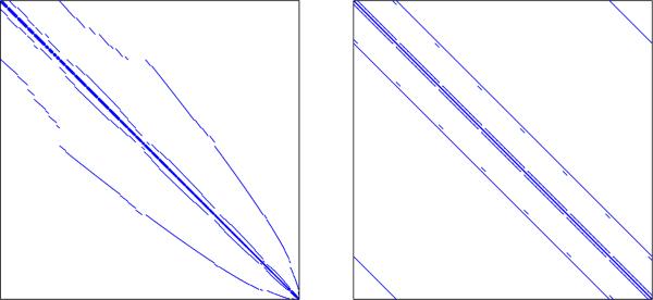
Laplacian matrices corresponding to the original data C^T C (left) and the augmented data C̃^T C̃ (right).

To address this issue, we introduce an augmentation matrix $\mathit{A}\in {\mathbb{R}}^{\tilde{p}\times p}$, whose rows are either the zero vector or an element from the trivial basis ${\left\{{\mathit{e}}_j\right\}}_{j=1}^p$, and has the property A^T A I_p. Furthermore, we define the augmented weight vector w̃ := Aw, wher A rectifies the irregularities in the coordinates of w (and x) by padding extra zero entries. This results in a new differencing matrix $\tilde{\mathit{C}}\in {\mathbb{R}}^{\tilde{e}\times \tilde{p}}$ for $\tilde{\mathit{w}}\in {\mathbb{R}}^{\tilde{p}}$, whose Laplacian matrix ${\tilde{\mathit{C}}}^T\tilde{\mathit{C}}\in {\mathbb{R}}^{\tilde{p}\times \tilde{p}}$ has a special structure known as block-circulant with circulant-blocks (BCCB) (see Fig. 1), which has important computational advantages.

Finally, by introducing a diagonal masking matrix $\mathit{B}\in {\{0,1\}}^{\tilde{p}\times \tilde{p}}$, we have ${\Vert \mathit{B}\tilde{\mathit{C}}\tilde{\mathit{w}}\Vert }_1={\Vert \mathit{C}\mathit{w}\Vert }_1$. Note that this masking strategy was adopted from the recent work of Allison et al. [18], and has the effect of removing artifacts introduced from data augmentation when computing the spatial penalty norm ∥·∥₁. This allows us to write out the FL-SVM problem (2) in the following equivalent form:

$$\underset{\mathit{w}\in {\mathbb{R}}^p}{\arg \min }\mathcal{L}\left(\mathit{Y}\mathit{X}\mathit{w}\right)+\lambda {\Vert \mathit{w}\Vert }_1+\lambda {\Vert \mathit{B}\tilde{\mathit{C}}\mathit{A}\mathit{w}\Vert }_1.$$ (7)

We propose the following variable splitting scheme to convert problem (7) into an equivalent constrained problem:

$$\begin{array}{c}\hfill \underset{\begin{array}{c}\hfill \mathit{w},{\mathit{v}}_1\hfill \\ \hfill {\mathit{v}}_2,{\mathit{v}}_3,{\mathit{v}}_4\hfill \end{array}}{\min }\mathcal{L}\left({\mathit{v}}_1\right)+\lambda {\Vert {\mathit{v}}_2\Vert }_1+\gamma {\Vert \mathit{B}{\mathit{v}}_3\Vert }_1\hfill \\ \hfill \mathrm{s}.\mathrm{t}.\mathit{Y}\mathit{X}\mathit{w}={\mathit{v}}_1,\mathit{w}={\mathit{v}}_2,\tilde{\mathit{C}}{\mathit{v}}_4={\mathit{v}}_3,\mathit{A}\mathit{w}={\mathit{v}}_4.\hfill \end{array}$$ (8)

Here, the correspondence with the ADMM formulation (3) is:

$$\begin{array}{c}\hfill \begin{array}{cc}\stackrel{‒}{\mathbf{f}}\left(\stackrel{‒}{\mathit{x}}\right)=\gamma {\Vert \mathit{B}{\mathit{v}}_3\Vert }_1,\hfill & \stackrel{‒}{\mathit{x}}={[{\mathit{w}}^T,{{\mathit{v}}_3}^T]}^T,\hfill \\ \stackrel{‒}{\mathit{g}}\left(\stackrel{‒}{\mathit{y}}\right)=\mathcal{L}\left({\mathit{v}}_1\right)+\lambda {\Vert {\mathit{v}}_2\Vert }_1,\hfill & \stackrel{‒}{\mathit{y}}={[{{\mathit{v}}_1}^T,{{\mathit{v}}_2}^T,{{\mathit{v}}_4}^T]}^T,\hfill \end{array}\hfill \\ \hfill \stackrel{‒}{A}=\left[\begin{array}{cc}\hfill \mathit{Y}\mathit{X}\hfill & \hfill 0\hfill \\ \hfill \mathit{I}\hfill & \hfill 0\hfill \\ \hfill 0\hfill & \hfill \mathit{I}\hfill \\ \hfill \mathit{A}\hfill & \hfill 0\hfill \end{array}\right],\stackrel{‒}{\mathit{B}}=\left[\begin{array}{ccc}\hfill -\mathit{I}\hfill & \hfill 0\hfill & \hfill 0\hfill \\ \hfill 0\hfill & \hfill -\mathit{I}\hfill & \hfill 0\hfill \\ \hfill 0\hfill & \hfill 0\hfill & \hfill -\tilde{\mathit{C}}\hfill \\ \hfill 0\hfill & \hfill 0\hfill & \hfill -\mathit{I}\hfill \end{array}\right].\hfill \end{array}$$ (9)

The dual variables corresponding to v₁, v₂, v₃, and v₄ are written in block form $\mathit{u}={[{{\mathit{u}}_1}^T,{{\mathit{u}}_2}^T,{{\mathit{u}}_3}^T,{{\mathit{u}}_4}^T]}^T$. Note that this formulation satisfies the sufficient conditions for the ADMM iterations (4)-(6) to converge, as functions f̄ and ḡ are convex, and matrices Ā and B̄ are full column-rank.

With the variable splitting scheme (8), the ADMM update for the primal variable x̄ (4) decomposes into subproblems

$$\begin{array}{cc}\hfill {\mathit{w}}^{(t+1)}& \leftarrow \underset{\mathit{w}}{\arg \min }\left\{{\Vert \mathit{Y}\mathit{X}\mathit{w}-({{\mathit{v}}_1}^{\left(t\right)}-{{\mathit{u}}_1}^{\left(t\right)})\Vert }_2^2+{\Vert \mathit{w}-({{\mathit{v}}_2}^{\left(t\right)}-{{\mathit{v}}_2}^{\left(t\right)})\Vert }_2^2+{\Vert \mathit{A}\mathit{w}-({{\mathit{v}}_4}^{\left(t\right)}-{{\mathit{u}}_4}^{\left(t\right)})\Vert }_2^2\right\}\hfill \\ \hfill {{\mathit{v}}_3}^{(t+1)}& \leftarrow \underset{{\mathit{v}}_3}{\arg \min }\gamma {\Vert \mathit{B}{\mathit{v}}_3\Vert }_1+\frac{\rho }{2}{\Vert {\mathit{v}}_3-(\tilde{\mathit{C}}{{\mathit{v}}_4}^{\left(t\right)}-{{\mathit{u}}_3}^{\left(t\right)})\Vert }_2^2\hfill \end{array}$$

whereas the updates for primal variable ȳ (5) are

$$\begin{array}{cc}\hfill \times {{\mathit{v}}_1}^{(t+1)}& \leftarrow \underset{{\mathit{v}}_1}{\arg \min }\mathcal{L}\left({\mathit{v}}_1\right)+\frac{\rho }{2}{\Vert {\mathit{v}}_1-(\mathit{Y}\mathit{X}{\mathit{w}}^{(t+1)}+{{\mathit{u}}_1}^{\left(t\right)})\Vert }_2^2\hfill \\ \hfill {{\mathit{v}}_2}^{(t+1)}& \leftarrow \underset{{\mathit{v}}_2}{\arg \min }\lambda {\Vert {\mathit{v}}_2\Vert }_1+\frac{\rho }{2}{\Vert {\mathit{v}}_2-({\mathit{w}}^{(t+1)}+{{\mathit{u}}_2}^{\left(t\right)})\Vert }_2^2\hfill \\ \hfill {{\mathit{v}}_4}^{(t+1)}& \leftarrow \underset{{\mathit{v}}_4}{\arg \min }\left\{{\Vert \tilde{\mathit{C}}{\mathit{v}}_4-({{\mathit{v}}_3}^{(t+1)}+{{\mathit{u}}_3}^{\left(t\right)})\Vert }_2^2+{\Vert {\mathit{v}}_4-(\mathit{A}{\mathit{w}}^{(t+1)}+{{\mathit{u}}_4}^{\left(t\right)}\Vert }_2^2\right\}.\hfill \end{array}$$

The closed form solutions for these are provided in Algorithm 1, which outlines the complete ADMM algorithm. We now demonstrate these updates can be carried out efficiently.

Algorithm 1.

ADMM algorithm for FL-SVM

1:	Initialize variables w, {v1, v2, v3, v4}, {u1, u2, u3, u4}
2:	Set t = 0, and precompute H–1 = (XTX + 2Ip)–1
3:	repeat
4:	w(t+1) ← H–1{XTYT [v1(t) – u1(t)] + [v2(t) – u2(t)] + AT [v4(t) – u4(t)]}
5:	${\left[{{\mathit{v}}_3}^{(t+1)}\right]}_i\leftarrow \{\begin{array}{cc}{\mathrm{Soft}}_{\gamma ∕\rho }\left({\left[\tilde{\mathit{C}}({{\mathit{v}}_4}^{\left(t\right)}-{{\mathit{v}}_3}^{\left(t\right)})\right]}_i\right)\hfill & \text{if}{\mathit{B}}_{i,i}=1\hfill \\ {\left[\tilde{\mathit{C}}({{\mathit{v}}_4}^{\left(t\right)}-{{\mathit{v}}_3}^{\left(t\right)})\right]}_i\hfill & \text{if}{\mathit{B}}_{i,i}=0\hfill \end{array}\phantom{\}}$
6:	${\left[{{\mathit{v}}_1}^{(t+1)}\right]}_j\leftarrow P{\mathrm{Prox}}_{\ell ∕\rho }\left({[\mathit{Y}\mathit{X}{\mathit{w}}^{(t+1)}+{{\mathit{u}}_1}^{\left(t\right)}]}_j\right)$
7:	[v2(t+1)]k ← Softλ/ρ ([w(t+1) + u2(t)]k)
8:	v4(t+1) ← (C̃TC̃ + Ip̃)–1 {C̃T[v3(t+1) + u3(t)] + Aw(t+1) + u4(t)} ▷ solve via FFT (10)
9:	u1(t+1) ← u1(t) + YXw(t+1) – v1(t+1)
10:	u2(t+1) ← u2(t) + w(t+1) – v2(t+1)
11:	u3(t+1) ← u3(t) + v3(t+1) – Cv4(t+1)
12:	u4(t+1) ← u4(t) + Aw(t+1) – v4(t+1)
13:	t ← t + 1
14:	until stopping criterion is met
	Note: [·]i, [·]j, [·]k in line 5-7 indicate vector elements

The inverse H⁻¹ for the w update (line 4 Alg. 1) can be converted into an n × n inversion problem using the matrix inversion Lemma, where n is on the order of a hundred in our application. The updates for v₁i, v₂, and v₃ (line 5-7 Alg. 1) are all separable across their coordinates and admit elementwise closed form solutions. Note Soft_r (t) := t(1 − τ|t|)₊ is the soft-threshold operator, and ${\mathrm{Prox}}_{\tau \ell }\left(t\right)$ is the proximal operator [19] corresponding to the hinge-loss:

$${\mathrm{Prox}}_{\tau \ell }\left(t\right)≔\{\begin{array}{cc}t\hfill & \text{if}t>1\hfill \\ 1\hfill & \text{if}1-\tau \le t\le 1\hfill \\ t+\tau \hfill & \text{if}t<-\tau \hfill \end{array}\phantom{\}}$$

Finally, the update for v₄ (line 8 Alg. 1) can be computed efficiently using the fast Fourier Transform (FFT). To suppress notations, let us define $\mathit{Q}≔{\tilde{\mathit{C}}}^T\tilde{\mathit{C}}+{\mathit{I}}_{\tilde{p}}$ and

$$\mathit{b}≔{\tilde{\mathit{C}}}^T[{{\mathit{v}}_3}^{\left(t\right)}+{{\mathit{u}}_3}^{\left(t\right)}]+\mathit{A}{\mathit{w}}^{(t+1)}+{{\mathit{u}}_4}^{\left(t\right)}.$$

As stated earlier, the Laplacian matrix ${\tilde{\mathit{C}}}^T\tilde{\mathit{C}}$ us a BCCB matrix, and consequently, the matrix Q is BCCB as well. It is well known that a BCCB matrix can be diagonalized as Q = U^H Λ U, where U is the (6-D) DFT matrix and is a diagonal matrix containing the (6-D) DFT coefficients of the first column of Q. As a result, the update for v₄ can be carried out efficiently using the (6-D) FFT

$${\mathit{Q}}^{-1}\mathit{b}=\left({\mathit{U}}^H{\Lambda }^{-1}\mathit{U}\right)\mathit{b}=\mathrm{ifft}(\mathrm{fft}\left(\mathit{b}\right)⨸\varphi ),$$ (10)

where fft and ifft denote the (6-D) FFT and inverse-FFT operation, ϕ is a vector containing the diagonal entries of Λ, and ⨸ indicates elementwise division.

We note that the ADMM algorithm was also used to solve FL-SVM in [20] under a different variable splitting setup. However, their application focuses on 1-D data, where the Laplacian matrix corresponding to their feature vector is tridiagonal with no irregularities present. Furthermore, the variable splitting scheme they propose requires an iterative algorithm to be used for one of the ADMM subproblems. In contrast, the variable splitting scheme and the data augmentation strategy we propose allow the ADMM subproblems to be decoupled in a way that all the updates can be carried out efficiently and non-iteratively in closed form.

3. EXPERIMENTS

In our experiments, we used the Center for Biomedical Research Excellence dataset made available by the Mind Research Network [21]. We analyzed resting state scans from 121 individuals consisting of 67 healthy controls 54 schiozophrenic subjects. For preprocessing details, we refer the readers to the extended version of our paper [22].

We compared the performance between the Elastic-net regularized SVM (EN-SVM) and FL-SVM; EN-SVM was also solved by ADMM, although the variable splitting and the optimization steps vary slightly from FL-SVM. The algorithms were terminated when the relative infeasibility $\frac{\Vert \stackrel{‒}{\mathit{A}}{\stackrel{‒}{\mathit{x}}}^{\left(t\right)}+\stackrel{‒}{\mathit{B}}{\stackrel{‒}{\mathit{y}}}^{\left(t\right)}\Vert }{\max \{\Vert \stackrel{‒}{\mathit{A}}{\stackrel{‒}{\mathit{x}}}^{\left(t\right)}\Vert ,\Vert \stackrel{‒}{\mathit{B}}{\stackrel{‒}{\mathit{y}}}^{\left(t\right)}\Vert \}}$ of the ADMM constraint (3) fell below 5 × 10⁻⁵ or the algorithm reached 400 iterations, and 10-fold cross-validation (CV) was used to evaluate the generalizability of the classifiers. All variables were initialized at zero.

A common practice for choosing the regularization parameters is to select the choice that gives the highest prediction accuracy. However, since our goal is the discovery and validation of imaging-based biomarkers, we need a model that not only good classification accuracy but also interpretability (i.e., sparsity). We found that the classifiers achieved a good balance between accuracy sparsity when approximately 4% of the features (2, 400) were selected out of p = 60, 031. More specifically, EN-SVM and FL-SVM achieved classification accuracies of 71.1% and 74.4% when the regularization parameters {λ, γ} were set at {2⁻⁹, 2⁻⁵ and 2⁻⁹, 2⁻¹²} and averages of 2180 and 2387 features were used across the CV folds. Hence, we further analyzed the classifiers obtained from these regularization parameters.

During CV, we learn a different weight vector for each partitioning of the dataset. In order to obtain a single representative weight vector, we re-trained the classifier using the entire dataset (121 subjects). For visualization and interpretation, we grouped the indices of these weight vectors according to the network parcellation scheme proposed by Yeo et al. in [23] (see Table 1), and reshaped them into 347 × 347 symmetric matrices with zeroes on the diagonal. Furthermore, we generated trinary representations of these matrices in order to highlight their support structures, where red, blue, and white denotes positive, negative, and zero entries respectively. The resulting matrices are displayed in Fig. 2.

Table 1.

Network parcellation of the brain proposed in [23].

Network Membership Table (× is “unlabeled”)
1. Visual	2. Somatomotor	3. Dorsal Attention
4. Ventral Attention	5. Limbic	6. Frontoparietal
7. Default	8. Striatum	9. Amygdala
10. Hippocampus	11. Thalamus	12. Cerebellum

Fig. 2.

Weight vectors learned using the full dataset. Top: heatmap of the weight vectors. Bottom: support structures of the weight vector, along with the degree plot of the nodes.

From these figures, one can observe that EN-SVM yields features that are scattered throughout the connectome space, which can be problematic for interpretation. On the other hand, FL-SVM recovered much more systematic sparsity patterns with multiple contiguous clusters, indicating that the predictive regions are compactly localized in the connectome space (e.g., see the rich connectivity patterns in the intra-visual and intra-cerebellum network). Moreover, FL-SVM recovers multiple highly connected hubs, which is an example of a spatially contiguous cluster in the connectome space. In order to emphasize this point, the bottom row in Fig. 2 also plots the degree of the nodes, i.e., the number of connections a node make with the rest of the network. This degree plot indicates that the frontoparietal network and cerebellum (among other regions) exhibited increased node degree, indicating diffuse connectivity alterations with other networks. Interestingly, these networks are among the most commonly implicated in schizophrenia [24].

4. CONCLUSION

We introduced a classification framework that explicitly accounts for the 6-D spatial structure in the FC via the fused Lasso SVM, which is solved using a novel alternating direction algorithm. We demonstrated that our method recovers sparse and highly interpretable feature patterns while maintaining predictive power, and thus could generate new insights into how psychiatric disorders impact brain networks.

REFERENCES

- 1.Atluri G, Padmanabhan K, Fang G, Steinbach M, Petrella JR, Lim K, MacDonald III A, Samatova NF, Doraiswamy PM, Kumar V. Complex biomarker discovery in neuroimaging data: Finding a needle in a haystack. Neuoimage: Clin. 2013;3(0):123–131. doi: 10.1016/j.nicl.2013.07.004. [DOI] [PMC free article] [PubMed] [Google Scholar]
- 2.Fox MD, Greicius M. Clinical applications of resting state functional connectivity. Front. Syst. Neurosci. 2010;419 doi: 10.3389/fnsys.2010.00019. [DOI] [PMC free article] [PubMed] [Google Scholar]
- 3.Castellanos FX, Martino AD, Craddock RC, Mehta AD, Milham MP. Clinical applications of the functional connectome. NeuroImage. 2013;80(0):527–540. doi: 10.1016/j.neuroimage.2013.04.083. [DOI] [PMC free article] [PubMed] [Google Scholar]
- 4.Varoquaux G, Craddock RC. Learning and comparing functional connectomes across subjects. NeuroImage. 2013 Oct;80(0):405–415. doi: 10.1016/j.neuroimage.2013.04.007. [DOI] [PubMed] [Google Scholar]
- 5.Candes EJ, Wakin MB. An introduction to compressive sampling. IEEE Trans. Signal Proc. Magazine. 2008;25(2):21–30. [Google Scholar]
- 6.Fan J, Lv J. A selective overview of variable selection in high dimensional feature space. Stat. Sinica. 2010;20(1):101–148. [PMC free article] [PubMed] [Google Scholar]
- 7.Tibshirani R. Regression shrinkage and selection via the Lasso. J. Roy. Stat. Soc. Ser. B. 1996;58(1):267–288. [Google Scholar]
- 8.Zou H, Hastie T. Regularization and variable selection via the Elastic Net. J. R. Stat. Soc. Ser. B Stat. Methodol. 2005;67:301–320. [Google Scholar]
- 9.Mairal J, Jenatton R, Obozinski G, Bach F. Convex and network flow optimization for structured sparsity. J. Mach. Learn. Res. 2011 Nov.12:2681–2720. [Google Scholar]
- 10.Micchelli CA, Morales JM, Pontil M. Regularizers for structured sparsity. Adv. Comput. Math. 2013;38(3):455–489. [Google Scholar]
- 11.Michel V, Gramfort A, Varoquaux G, Eger E, Thirion B. Total variation regularization for fMRI-based prediction of behavior. IEEE Trans. Med. Imaging. 2011;30(7):1328–1340. doi: 10.1109/TMI.2011.2113378. [DOI] [PMC free article] [PubMed] [Google Scholar]
- 12.Grosenick L, Klingenberg B, Katovich K, Knutson B, Taylor JE. Interpretable whole-brain prediction analysis with GraphNet. NeuroImage. 2013;72(0):304–321. doi: 10.1016/j.neuroimage.2012.12.062. [DOI] [PubMed] [Google Scholar]
- 13.Tibshirani R, Saunders M, Rosset S, Zhu J, Knight K. Sparsity and smoothness via the fused Lasso. J. R. Stat. Soc. Ser. B Stat. Methodol. 2005;67(1):91–108. [Google Scholar]
- 14.Boyd S, Parikh N, Chu E, Peleato B, Eckstein J. Distributed optimization and statistical learning via the alternating direction method of multipliers. Found. Trends Mach. Learn. 2011;3:1–122. [Google Scholar]
- 15.Cortes C, Vapnik V. Support-vector networks. Mach. Learn. 1995;20(3):273–297. [Google Scholar]
- 16.Mota JFC, Xavier JMF, Aguiar PMQ, Püschel M. A proof of convergence for the alternating direction method of multipliers applied to polyhedral-constrained functions. arXiv:1112.2295. 2011 [Google Scholar]
- 17.Afonso MV, Bioucas-Dias JM, Figueiredo MAT. Fast image recovery using variable splitting and constrained optimization. IEEE Trans. Image Proc. 2010;19(9):2345–2356. doi: 10.1109/TIP.2010.2047910. [DOI] [PubMed] [Google Scholar]
- 18.Allison MJ, Ramani S, Fessler JA. Accelerated regularized estimation of MR coil sensitivities using Augmented Lagrangian methods. IEEE Trans. Med. Imaging. 2013;32(3):556–564. doi: 10.1109/TMI.2012.2229711. [DOI] [PMC free article] [PubMed] [Google Scholar]
- 19.Combettes P, Wajs V. Signal recovery by proximal forward-backward splitting. Multiscale Modeling & Simulation. 2005;4(4):1168–1200. [Google Scholar]
- 20.Ye GB, Xie X. Split bregman method for large scale fused lasso. Comput. Stat. Data Anal. 2011;55(4):1552–1569. [Google Scholar]
- 21.The Mind Research Network (MRN) The Center for Biomedical Research Excellence (COBRE) http://fcon_1000.projects.nitrc.org/indi/retro/cobre.html.
- 22.Watanabe T, Kessler D, Scott C, Angstadt M, Sripada C. Disease Prediction based on Functional Connectomes using a Spatially-Informed Fused Lasso Support Vector Classiffier. arXiv:1310.5415. 2013 doi: 10.1016/j.neuroimage.2014.03.067. [DOI] [PMC free article] [PubMed] [Google Scholar]
- 23.Yeo BTT, Krienen FM, Sepulcre J, Sabuncu MR, Lashkari D, Hollinshead M, Roffman JL, Smoller JW, Zöllei L, Polimeni JR, Fischl B, Liu H, Buckner RL. The organization of the human cerebral cortex estimated by intrinsic functional connectivity. J. Neurophysiol. 2011;106(3):1125–65. doi: 10.1152/jn.00338.2011. [DOI] [PMC free article] [PubMed] [Google Scholar]
- 24.Fornito Alex, Zalesky Andrew, Pantelis Christos, Bullmore Edward T. Schizophrenia, neuroimaging and connectomics. NeuroImage. 2012;62(4):2296–2314. doi: 10.1016/j.neuroimage.2011.12.090. [DOI] [PubMed] [Google Scholar]