Dynamic causal modelling for functional near-infrared spectroscopy

Abstract

Functional near-infrared spectroscopy (fNIRS) is an emerging technique for measuring changes in cerebral hemoglobin concentration via optical absorption changes. Although there is great interest in using fNIRS to study brain connectivity, current methods are unable to infer the directionality of neuronal connections. In this paper, we apply Dynamic Causal Modelling (DCM) to fNIRS data. Specifically, we present a generative model of how observed fNIRS data are caused by interactions among hidden neuronal states. Inversion of this generative model, using an established Bayesian framework (variational Laplace), then enables inference about changes in directed connectivity at the neuronal level. Using experimental data acquired during motor imagery and motor execution tasks, we show that directed (i.e., effective) connectivity from the supplementary motor area to the primary motor cortex is negatively modulated by motor imagery, and this suppressive influence causes reduced activity in the primary motor cortex during motor imagery. These results are consistent with findings of previous functional magnetic resonance imaging (fMRI) studies, suggesting that the proposed method enables one to infer directed interactions in the brain mediated by neuronal dynamics from measurements of optical density changes.

Highlights

• •We apply Dynamic Causal Modelling (DCM) to functional NIRS (fNIRS) data.
• •DCM-fNIRS enables inference about directed connectivity at the neuronal level.
• •An analysis is performed using fNIRS data acquired during motor imagery and execution.
• •Results are consistent with findings of previous fMRI studies.

Introduction

Functional near-infrared spectroscopy (fNIRS) is a noninvasive method for monitoring hemodynamic changes in the brain (Jobsis, 1977; Villringer et al., 1993; Hoshi, 2007; Ferrari and Quaresima, 2012; Scholkmann et al., 2014). fNIRS works by shining near-infrared light in the spectral range between 650 and 950 nm from fiber-optic emitters placed on the scalp. Because the absorption of chromophores in tissue is relatively low within this spectral range, near-infrared light can propagate several centimeters through tissue. Changes in light photon density reaching the detectors correspond to changes in the optical properties of the tissue, reflecting changes in oxygenated and deoxygenated hemoglobin (HbO and HbR). The loss of light levels can then be used to calculate the changes in hemoglobin concentrations in underlying brain regions (Delpy et al., 1988). As neuronal processes require extra delivery of oxygen, this provides a marker of underlying neuronal activity.

fNIRS has many advantages that make it highly useful in cognitive and clinical neuroscience studies. Compared to other imaging modalities, such as functional magnetic resonance imaging (fMRI), fNIRS is mobile and compact, and the data acquisition is quiet. Furthermore, as compared to fMRI, fNIRS provides a more direct measure of changes in HbO, HbR, and total hemoglobin (HbT), and the time series are sampled at high temporal resolution. It has therefore proved to be an effective tool for studying physiological mechanisms in the healthy brain and in cerebrovascular disease (Highton et al., 2010; Wolf et al., 2012; Obrig, 2014). It is also finding unique applications in clinical areas, including bedside monitoring of infants, and studies of auditory and language systems (Lloyd-Fox et al., 2010; Eggebrecht et al., 2014).

There is currently a surge of interest in characterizing brain connectivity using fNIRS. Recent fNIRS studies have assessed the coupling between brain regions in terms of a measure of functional connectivity (Homae et al., 2010; Sasai et al., 2011) and effective connectivity (Im et al., 2010; Yuan, 2013). Specifically, Homae et al. (2010) explored developmental changes of brain networks in early infancy, using functional connectivity defined as temporal correlation between pairs of fNIRS measurements. Sasai et al. (2011) investigated the frequency-specific characteristics of functional connectivity based on spontaneous oscillation in the low-frequency range in HbO and HbR signals. However, functional connectivity does not provide any insight into the directed causal interactions among brain regions underlying cognitive processing. To address this shortcoming, Im et al. (2010) and Yuan (2013) applied Granger causality analysis to fNIRS data, which provides estimation of the directed functional connectivity between brain regions. The analyses of both functional connectivity and effective (via Granger causality) connectivity are usually performed at the level of measured hemodynamic signals, such as HbO, HbR, and HbT responses (White et al., 2009; Im et al., 2010; Homae et al., 2010; Sasai et al., 2011; Yuan, 2013). However, connectivity estimates at the level of hemodynamic measurements are not direct measures of connectivity changes at the neuronal level, because the hemodynamic response to neuronal activation depends on the balance of the changes in cerebral blood flow and oxidative metabolism, and also on the changes in cerebral blood volume (Fox and Raichle, 1986; Buxton, 2012). This complex interplay between processes can cause functional connectivity to differ with the type of hemoglobin changes (e.g., HbO and HbR), while underlying interactions between neuronal populations do not vary (Lu et al., 2010). This highlights the importance of estimating causal influences among neuronal populations, referring to a biophysical model of how neuronal activity is transformed into fNIRS measurements.

Several fNIRS studies have used biophysical models relating blood inflow to HbO and HbR changes, or neuronal activity to HbO and HbR changes during brain activation. Specifically, Cui et al. (2010) generated synthetic HbO and HbR responses induced by blood inflow using the Balloon model in a study that investigated the effect of head motion on the fNIRS signal. Dubeau et al. (2012) recovered neuronal inputs from hemodynamic measurements by deconvolving the extended Balloon model (Friston et al., 2000), and showed significant correlation between estimated neural inputs and measurements of local field potentials and multiunit activity. However, to our knowledge, there have been no studies focusing on model-based estimation of neuronal interaction among multiple regions from the optical density changes using fNIRS.

In this paper, we apply Dynamic Causal Modelling (DCM) to fNIRS data, to estimate effective connectivity at the neuronal level from the measurement of optical density changes. Effective connectivity is defined as the (model-based) influence of one (neuronal) system on another. DCM is a framework for fitting differential equation or state space models of neuronal activity to brain imaging data using Bayesian inference (Friston et al., 2003). There is now a library of DCMs and variants differ according to their level of biological realism and the data features which they explain. The DCM approach can be applied to fMRI (Friston et al., 2003, 2014), electroencephalographic (EEG), and Magnetoencephalographic (MEG) data (Moran et al., 2007; Penny et al., 2009; Daunizeau et al., 2009b).

This paper extends the DCM approach to fNIRS. Because the variational Bayesian estimation algorithm is the same as that used for DCMs for other imaging modalities, this paper focuses on development of a generative model of how observed fNIRS data are caused by the interactions among hidden neuronal states. In particular, we extend the neurodynamic and hemodynamic models used for DCM-fMRI analysis (Friston et al., 2003) to additionally include the total hemoglobin state (Cui et al., 2010), and optics model that describes the detected optical density changes as a linear combination of light absorption changes due to HbO and HbR (Delpy et al., 1988; Arridge, 1999). The model is further augmented by including spatially extended hemodynamic sources (Shmuel et al., 2007) and pial vein contamination effects (Gagnon et al., 2012). In short, the proposed method allows fNIRS to be used for making inference about changes in directed connectivity at the neuronal level.

This paper is structured as follows: In the Methods section we first describe a generative model of fNIRS data, and then describe the model optimization procedure for estimating the connectivity parameters from this data. In the Results section we provide an illustrative analysis using fNIRS data acquired during the motor imagery and motor execution tasks. In the Discussion section we discuss future extensions of the proposed method.

Methods

The generative model for fNIRS data comprises three components: (i) neurodynamics describing neural activity in terms of inter-regional interactions and its experimentally induced modulation (Friston et al., 2003), (ii) hemodynamics linking neural activity with the changes in total hemoglobin, and deoxy-hemoglobin based on the Balloon model (Friston et al., 2000; Buxton et al., 2004; Cui et al., 2010), and (iii) optics relating the hemodynamic sources to optical density changes (Delpy et al., 1988; Arridge, 1999). A schematic of the generative model is summarized in Fig. 1. The following subsections describe each of these components. These are followed by sections on computing the optical sensitivity matrix and confounding effects that underlie the optical model, and a section on model estimation.

Fig. 1.

Schematic of the generative model of fNIRS data. The neurodynamic equation uses linear differential equations and a single state variable per region describing neural activity. Coupling parameter matrices A, Bⁱ, and C represent the average connectivity among regions, the modulation of effective connectivity by experimental manipulation, and the influence of inputs on regions, respectively. The hemodynamic equation uses the Balloon model and its extensions to describe how neural activity causes a change in a flow inducing signal which in turn causes an increase in blood flow with concomitant changes in relative blood volume and deoxy-hemoglobin. The optics equation uses a sensitivity matrix, S, describing how changes in hemodynamic sources cause changes in optical measurements. Potential pial vein contamination of the fNIRS measurements is corrected using matrices W_H and W_Q. Spatially distributed hemodynamic source is generated using Gaussian spatial smoothing kernel K.

Neurodynamics

The neurodynamics are described by the following multivariate differential equation

$$\begin{array}{l}{\dot{z}}_t={\Im }_t{z}_t+C{u}_t\\ {\Im }_t=A+{\displaystyle \sum _{i=1}^M}{u}_t\left(i\right)B^i\text{,}\end{array}$$ (1)

where t indexes continuous time and the dot notation denotes a time derivative. The entries in z correspond to neuronal activity in j = 1,…,L cortical source regions, and u(i) is the ith of M experimental inputs. An [L × L] matrix, ℑ, denotes the effective connectivity between and within regions, and an [L × M] matrix, C, defines a set of experimental input connections that specify which inputs are connected to which regions.

The effective connectivity ℑ is characterized by an [L × L] connectivity matrix, A, that specifies which regions are connected in the absence of exogenous or experimental input and whether these connections are unidirectional or bidirectional. We also define an [L × L] modulatory matrix, Bⁱ, that specifies which intrinsic connections can be changed as a result of input i. Usually, the Bⁱ parameters are of greatest interest — as these describe how connections among brain regions respond to experimental manipulations. For example, in the application in this paper we show how connections among regions in the motor system are modulated by motor imagery.

The overall specification of input, intrinsic and modulatory connectivity comprises our assumptions about model structure. This in turn represents a scientific hypothesis about the structure of the large-scale neuronal network mediating the underlying function.

The above neurodynamical model is bilinear, and deterministic, and has a single-state variable per region. However, as we can build on developments made in DCM for fMRI, these models are readily extended to the nonlinear and stochastic cases (Stephan et al., 2008; Daunizeau et al., 2009a). In future publications we will also explore the use of richer dynamical models, employing for example two-state variables per region (Marreiros et al., 2008).

To enforce constraints on the parameters being estimated, we make use of latent variables. For example, the use of latent variables, Ã_ij and ${\tilde{B}}_{ij}$, ensures that self connections, ℑ_ii, are negative with a typical value of 0.5: ${\Im }_{ii}=-0.5exp\left({\tilde{A}}_{ii}+{\displaystyle {\sum }_k}{u}_t\left(k\right){\tilde{B}}_{ii}^k\right)$. Thus, although Ã_ii and ${\tilde{B}}_{ii}$ have Gaussian priors (see the Priors, estimation, and model selection section) and can be positive or negative, ℑ_ii will be strictly negative. For the off-diagonal terms, we have no such constraints, i.e. A_ij = Ã_ij, $B_{ij}={\tilde{B}}_{ij}$. Overall, the neuronal parameters are ${\theta }_n=\left\{\tilde{A},\tilde{B},C\right\}$.

Hemodynamics

The hemodynamic model involves a set of hemodynamic state variables, state equations and hemodynamic parameters, θ_h. Neuronal activity in source region j, z_j, causes an increase in vasodilatory signal s_j that is subject to autoregulatory feedback, and inflow f_i,in responds in proportion to this (Friston et al., 2000)

$$\begin{array}{l}{\dot{s}}_j=z_j-{\kappa }_j{s}_j-{\gamma }_j\left(f_{j,\mathit{in}}-1\right)\\ {\dot{f}}_{j,\mathit{in}}=s_j\text{,}\end{array}$$ (2)

where κ_j is the rate of signal decay, and γ_j is the rate of autoregulatory feedback by blood flow.

The rate of blood volume v_j (Buxton et al., 1998) and total hemoglobin concentration p_j (Cui et al., 2010) changes as

$$\begin{array}{l}{\tau }_j{\dot{v}}_j=f_{j,\mathit{in}}-f_{j,\mathit{out}}\\ {\tau }_j{\dot{p}}_j=\left(f_{j,\mathit{in}}-f_{j,\mathit{out}}\right)\frac{p_j}{v_j}\text{,}\end{array}$$ (3)

where the first equation describes the filling of the venous ‘Balloon’ until inflow equals outflow, f_j,out, which happens with the transit time τ_j.

The rate of deoxy-hemoglobin q_j changes is modeled as the delivery of deoxy-hemoglobin into the venous compartment minus that expelled (Buxton et al., 1998)

$$\begin{array}{l}{\tau }_j{\dot{q}}_j=f_{j,\mathit{in}}\frac{E\left(f_{j,\mathit{in}},\rho \right)}{\rho }-f_{j,\mathit{out}}\frac{q_j}{v_j}\\ E\left(f,\rho \right)=1-{\left(1-\rho \right)}^{1/f}\end{array}$$ (4)

where E(f, ρ) is the proportion of oxygen extracted from the blood and ρ is the resting oxygen extraction fraction.

In the steady-state the outflow is modeled as a power of blood volume (Grubb et al., 1974). However, in the transient state the blood volume changes often lag behind the blood flow changes. To address this dynamic relationship, the outflow model is further augmented by including viscoelastic time parameter τ_j,v (Buxton et al., 2004):

$$f_{j,\mathit{out}}=v_j^{1/\alpha }+{\tau }_{j,v}{\dot{v}}_j\text{,}$$ (5)

where α is Grubb's exponent (Grubb et al., 1974), and τ_j,v describes an additional resistance of venous blood vessels to rapid blood volume changes.

Four of the hemodynamic parameters are estimated from each source activity: ${\theta }_h=\left\{{\tilde{\kappa }}_j,{\tilde{\gamma }}_j,{\tilde{\tau }}_j,{\tilde{\tau }}_{j,v}\right\}$. The use of latent variables ensures that estimated hemodynamic parameters are within a physiologically realistic range:

$$\begin{array}{l}{\kappa }_j=0.64exp\left({\tilde{\kappa }}_j\right)\\ {\gamma }_j=0.32exp\left({\tilde{\gamma }}_j\right)\\ {\tau }_j=2exp\left({\tilde{\tau }}_j\right)\\ {\tau }_{j,v}=2exp\left({\tilde{\tau }}_{j,v}\right)\text{.}\end{array}$$ (6)

The other parameters are fixed to α = ρ = 0.32 in accordance with previous work (Stephan et al., 2007).

The viscoelastic time constant τ_j,v ranges from 0 to 30 s (Buxton et al., 2004). However, it is known from high field fMRI studies (Yacoub et al., 2005; Jin and Kim, 2008) that τ_j,v can decrease as one moves from deep to more superficial cortical layers. fNIRS measures signal mainly from the superficial cortical layers, potentially reflecting tissue properties from deeper layers through draining veins. We therefore used, a broad prior over τ_j,v having a mean of 2 with prior standard deviation of latent variable ${\tilde{\tau }}_{j,v}=1$ in Eq. (6), so that three standard deviations (i.e., 2 exp(3) = 40.17) can cover the physiological ranges.

Optics

A fNIRS optode array comprises N_s optical sources (emitters) and N_d optical detectors which are paired up to form i = 1, …, N channels. In principle, all optical channels are sensitive to all neuronal sources. In practice, the sensitivity of channels to sources is governed by the sensitivity matrix (see below). It provides N channel measurements of optical density changes at time t and wavelength λ₁, and N at λ₂. These are written as the [N × 1] vectors y(λ₁) and y(λ₂). These channel measurements are then related to the [L × 1] vectors of HbO and HbR, ΔH_c and ΔQ_c, in the L cortical source regions of interest as

$$\left[\begin{array}{c}\hfill y\left({\lambda }_1\right)\hfill \\ \hfill y\left({\lambda }_2\right)\hfill \end{array}\right]=\left[\begin{array}{cc}\hfill {ϵ}_H\left({\lambda }_1\right)W_{H}S\left({\lambda }_1\right)\hfill & \hfill {ϵ}_Q\left({\lambda }_1\right)W_{Q}S\left({\lambda }_1\right)\hfill \\ \hfill {ϵ}_H\left({\lambda }_2\right)W_{H}S\left({\lambda }_2\right)\hfill & \hfill {ϵ}_Q\left({\lambda }_2\right)W_{Q}S\left({\lambda }_2\right)\hfill \end{array}\right]\left[\begin{array}{c}\hfill \mathrm{\Delta }{H}_c\hfill \\ \hfill \mathrm{\Delta }{Q}_c\hfill \end{array}\right]\text{,}$$ (7)

with

$$\begin{array}{l}\mathrm{\Delta }{H}_c=\mathrm{\Delta }{P}_c-\Delta Q_c\\ \mathrm{\Delta }{P}_c=P_0\cdot p-1\\ \mathrm{\Delta }{Q}_c=Q_0\cdot q-1\text{,}\end{array}$$

where ϵ_H and ϵ_Q are the extinction coefficients for HbO and HbR; S is the [N × L] sensitivity matrix; p and q are HbT and HbR normalized to their baseline concentrations P₀ and Q₀ = P₀(1 − SO₂) where SO₂ is the baseline oxygenation saturation; and W_H and W_Q are [N × N] matrices for correcting pial vein contamination of fNIRS measurements:

$$\begin{array}{l}{W}_H=diag\left[\frac{1}{{\omega }_{1,H}},\dots ,\frac{1}{{\omega }_{N,H}}\right],\\ W_Q=diag\left[\frac{1}{{\omega }_{1,Q}},\dots ,\frac{1}{{\omega }_{N,Q}}\right]\text{,}\end{array}$$ (8)

where ω is the ratio of cortical tissue signal over the total activated signal originating from cortical tissue and pial vein: $\omega =\frac{\mathrm{cortical}}{\mathrm{cortical}+\mathrm{pial}}$ (Gagnon et al., 2012).

Two of the optics parameters are estimated from the data for each channel location: ${\theta }_p=\left\{{\tilde{\omega }}_{i,H},{\tilde{\omega }}_{i,Q}\right\}$. The other parameters in Eq. (7) are fixed to P₀ = 71 μM (Yücel et al., 2012), and SO₂ = 0.65 (Boas et al., 2003). The use of latent variables ensures that the estimated cortical fraction of fNIRS measurements is within a physiologically realistic range:

$$\begin{array}{l}{\omega }_{i,H}=0.5exp\left({\tilde{\omega }}_{i,H}\right)\\ {\omega }_{i,Q}=0.5exp\left({\tilde{\omega }}_{i,Q}\right)\text{.}\end{array}$$ (9)

The optical density measurement, y, is affected by the signals arising from both cerebral and extracerebral (e.g., pial vasculature and skin) regions, since the fNIRS signal is integrated through the different superficial layers of the head (Liebert et al., 2004; Dehaes et al., 2011; Gagnon et al., 2012; Kirilina et al., 2012) Specifically, Gagnon et al. (2012) showed that evoked oxygenation changes in the cortex can propagate through the pial veins at the surface of the cortex, which leads to different cortical weighting factors for HbO and HbR (ω_H ≈ 0.76, ω_Q ≈ 0.19). We set prior means of ω_i,H and ω_i,Q to 0.5 (Eq. (9)), and then estimated these values from data.

The i, jth element of the sensitivity matrix, S_i,j at wavelength λ in Eq. (7) is given by

$$S_{i,j}\left(\lambda \right)=\frac{G\left(r_{i,s},r_{j,h}\right)G\left(r_{j,h},r_{i,d}\right)}{G\left(r_{i,s},r_{i,d}\right)}$$ (10)

where r_i,s and r_i,d are the optical source and optical detector positions for the ith of N channel measurements, and r_j,h is the hemodynamic source position in the jth brain region of interest. The quantity G(r₁, r₂) is Green's function of the photon fluence at position r₂ from a source at r₁. S_i,j is the ratio of light received indirectly (by detector d_i from source s_i) via scattering from hemodynamic source h_j versus that received directly, which corresponds to the effective pathlength of detected photons for the ith channel measurement in the jth hemodynamic source. In practice, the sensitivity matrix can be estimated by simulating photon migration through the head and brain based on a Monte Carlo method (Wang et al., 1995; Boas et al., 2002; Fang, 2010) or finite element methods (Dehghani et al., 2009). These computations require a structural Magnetic Resonance Image (sMRI) of the subject's head and brain. However, when the subject-specific sMRI is not available, it is also possible to use a canonical sMRI (see Cooper et al., 2012; Ferradal et al., 2014 for a comparison). In addition, given a set of standard optode positions and a canonical cortical surface, Green's functions can be pre-computed. This is analogous to the pre-computation of a standard lead field model for M/EEG source reconstruction (or DCM for M/EEG). Thus, users of DCM for fNIRS can use these standard forward models, thus saving a large amount of computation time.

Computing the sensitivity matrix

In this study, we used the mesh-based Monte Carlo simulation software (MMC, Fang (2010)) to estimate Green's function of the photon fluence, and then calculate a matrix of the sensitivity to the absorption coefficient changes S in Eq. (10). Specifically, given a 3D finite-element mesh generated from a canonical sMRI (Holmes et al., 1998; Fang and Boas, 2009), we launch 10⁸ photons from the optical source position of each channel r_s to estimate Green's functions, G(r_s, r_h) and G(r_s, r_d), from the position of optical source r_s into the positions of the hemodynamic sources r_h and the position of optical detector r_d, respectively. We also launch 10⁸ photons from the optical detector position of each channel r_d to estimate Green's function G(r_d, r_h), which, according to the reciprocity theorem (Arridge, 1999), is equivalent to G(r_h, r_d). Since tissue-type specific labeling of optical properties provides a more accurate light model than assuming homogeneous optical properties (Heiskala et al., 2009), each tetrahedral volume element is labeled by tissue type, and assigned optical properties as summarized in Table 1. Optical properties for the scalp/skull, cerebrospinal fluid (CSF), gray matter, and white matter are identical to those used in the literature (Fang, 2010; Eggebrecht et al., 2012).

Table 1.

Optical properties of scalp & skull, cerebrospinal fluid (CSF), gray matter, and white matter for Monte Carlo simulation. Absorption coefficients μ_a and scattering coefficients μ_s for various brain tissue types are based on those used in Eggebrecht et al. (2012). Anisotropy factor g and refraction index n are based on those used in Fang (2010). The units of μ_a and μ_s are mm^− 1.

	760 nm		850 nm		Anisotropy factor	Refraction index
	μa	μs	μa	μs	g	n
Scalp & skull	0.0143	7.6364	0.0164	6.7273	0.89	1.37
CSF	0.0040	2.7273	0.0040	2.7273	0.89	1.37
Gray matter	0.0180	7.5991	0.0192	6.1145	0.89	1.37
White matter	0.0167	10.8255	0.0208	9.1882	0.84	1.37

Distributed sources

In Eq. (7), we have modeled each hemodynamic signal as a point source which produces a hemodynamic response at a single specified anatomical location. However, it is also possible to consider hemodynamic responses as being spatially extended. Assuming that the spatial point spread functions of hemodynamic responses are approximately Gaussian (Shmuel et al., 2007), the spatially distributed hemodynamic source can be specified by convolving the temporal response with a Gaussian spatial kernel whose width can be estimated during model inversion. Hemodynamic activity at source location r_l is then given by

$$\begin{array}{l}\Delta H_c\left(r_l,r_j\right)=K\left(r_l,r_j\right)\Delta H_c\left(r_j\right)\\ \Delta Q_c\left(r_l,r_j\right)=K\left(r_l,r_j\right)\Delta Q_c\left(r_j\right)\\ K\left(r_l,r_j\right)=exp\left(\frac{-{\left|r_l-r_j\right|}^2}{2{\sigma }^2\left(r_j\right)}\right)\text{,}\end{array}$$ (11)

where r_j is the center of the hemodynamic kernel, r_l is the position in the Montreal Neurological Institute (MNI) space, K(r_l, r_j) is the Gaussian spatial smoothing kernel at position r_l from position r_j, distance between the lth distributed source and jth point source, |r_l − r_j| ≤ d_j,max, and bandwidth of kernel, $\sigma \left(r_j\right)=d_{j,max}/2\sqrt{2\ln 2}$. Here, the maximum distance between point and distributed sources, d_j,max, is estimated, and the use of a latent variable, ${\tilde{d}}_{j,max}$, allows the estimate of d_j,max to vary about 4 mm as

$$d_{j,max}=4exp\left({\tilde{d}}_{j,max}\right)\text{.}$$ (12)

when using distributed sources, we have three optics parameters to estimate: ${\theta }_p=\left\{{\tilde{\omega }}_{i,H},{\tilde{\omega }}_{i,Q},{\tilde{d}}_{j,max}\right\}$.

Confounds

One of the challenges for fNIRS-based connectivity studies is that the fNIRS signal can be significantly contaminated with systemic physiological interference. Such systemic physiological noise, induced by heart beat, respiration, and blood pressure variations, may interfere with the estimation of fNIRS-based connectivity (Boas et al., 2004; Kirilina et al., 2012). However, recent fNIRS studies have shown that this physiological interference can be effectively removed by regressing out the global signal (Mesquita et al., 2010), physiological noises generated from different frequency bands of fNIRS data (Tong et al., 2011), or a signal derived from superficial scalp measurements using a short source–detector separation channel (White et al., 2009; Saager et al., 2011; Gagnon et al., 2011; Gagnon et al., 2014; Goodwin et al., 2014).

In our approach, very low-frequency confounds (c.f., drift terms in fMRI convolution models) were removed from the fNIRS channel measurements, by using a high-pass filter with a cutoff frequency of 0.008 Hz. Physiological noises, including respiration and cardiac pulsation, were then removed by using a band-stop filter with cutoff frequencies of [0.12 0.35] and [0.7 1.5] Hz, respectively. In addition, the forward model in Eq. (13) produced by integrating the neuronal and hemodynamic state equations can be extended by adding the confounding effects X (see below). We therefore used a discrete cosine transform set with cutoff periods of [8 12] seconds and a constant term in X, to model Mayer waves (Obrig et al., 2000) and baseline shift. Confounding effects on the observed signal were then estimated and removed during model inversion. Note that additional measurements of systemic confounds e.g., changes in blood pressure (Minati et al., 2011; Tachtsidis et al., 2009; Takahashi et al., 2011) and arterial partial pressure of CO₂ (Scholkmann et al., 2013) can also be used in the proposed method, which may enhance the efficiency of effective connectivity estimates.

Priors, estimation, and model selection

The neurodynamic, hemodynamic, and optics parameters can be concatenated in a vector of free parameters, θ = {θ_n, θ_h, θ_p}. The DCM parameters are then estimated from the data, y, using Bayesian inference, where competing hypotheses or models are compared using their evidence (Penny, 2012).

For any given parameters θ, model predictions, g(θ) can be generated by integrating the forward equations as described in Friston et al. (2003). The observed data y is then modeled as

$$y=g\left(\theta ,m\right)+X\beta +e\text{,}$$ (13)

where X contains confounding effects, β is the associated parameter vector, and e is the zero mean additive Gaussian noise with covariance C_y. The error covariances are assumed to decompose into terms of the form C_y⁻¹ = ∑_iexp(λ_i)Q_i where Q_i are the known precision basis functions. The likelihood of the data is therefore

$$p\left(y\left|\theta ,\lambda ,m\right)\right)=N\left(y;g\left(\theta ,m\right),C_y\right)\text{.}$$ (14)

The priors, p(θ|m), assume to be Gaussian. The priors used in this paper correspond to those implemented in SPM12 software, and their mean and variance are summarized in Table 2. We also use a normal prior p(λ|m) over the log error precision, λ.

Table 2.

Prior mean and standard deviation (SD) on neurodynamic and hemodynamic parameters. i and j index source regions, k indexes an experimental input, l indexes sensor region, and $\tilde{X}$ denotes the latent variables from which X is derived.

Parameter	Description	Prior mean	Prior SD
Ãij	Extrinsic connection in the absence of input	0.0078	0.25
Ãii	Intrinsic connection in the absence of input	0	0.25
${\tilde{B}}_{ij}^k$	Extrinsic connection modulated by input	0	1
${\tilde{B}}_{ii}^k$	Intrinsic connection modulated by input	0	1
Cij	Influence of input on regional activity	0	1
${\tilde{\kappa }}_j$	Signal decay rate	0	0.05
${\tilde{\gamma }}_j$	Rate of autoregulatory feedback	0	0.05
${\tilde{\tau }}_j$	Transit time	0	0.05
${\tilde{\tau }}_{j,v}$	Viscoelastic time	0	1
${\tilde{d}}_{jmax}$	Spatial kernel width	0	0.05
${\tilde{\omega }}_{l,H}$	Cortical fraction of HbO	0	0.22
${\tilde{\omega }}_{l,Q}$	Cortical fraction of HbR	0	0.22

The posterior distribution is then estimated using a variational Laplace (VL) method (Friston et al., 2007). Specifically, the VL algorithm assumes an approximate posterior density of the following factorized form

$$q\left(\theta ,\lambda \left|y,m\right)\right)=q\left(\theta \left|y,m\right)\right)q\left(\lambda \left|y,m\right)\right)\text{,}$$ (15)

where q(θ|y, m) = N(θ; m_θ, S_θ), and q(λ|y, m) = N(λ; m_λ, S_λ). The DCM parameters θ and hyperparameters λ of these approximate posteriors are then iteratively updated so as to minimize the Kullback–Leibler (KL)-divergence between the true and approximate posteriors. This is a standard approach in Bayesian statistics and machine learning (Bishop, 2006).

The structure of a DCM is defined by the connectivity matrices A, B, and C. Different models can be compared using the evidence for each model. This can be thought of as a second-level of Bayesian inference. The model evidence is given by

$$p\left(y\left|m\right)\right)={\displaystyle \int }{\displaystyle \int }p\left(y\left|\theta ,\lambda ,m\right)\right)p\left(\theta \left|m\right)\right)p\left(\lambda \left|m\right)\right)\mathit{d\theta d\lambda }\text{.}$$ (16)

While the model evidence is not straightforward to compute, it is possible to place a lower bound on the log model evidence of the following form

$$logp\left(y\left|m\right)\right)=F\left(m\right)+KL\left[q\left(\theta ,\lambda \left|m\right)\right)\left.‖p\left(\theta ,\lambda \left|y,m\right)\right)\right)\right]\text{,}$$ (17)

where F(m) is known as the negative variational free energy and the last term is the Kullback–Leibler (KL) distance between the true posterior density, p(θ, λ|y, m), and an approximate posterior q(θ, λ|m). Free energy is estimated as above using the Laplace approximation (Friston et al., 2007). Once the evidence has been computed, Bayesian inference at the model level can then be implemented using the Bayes rule:

$$p\left(m\left|y\right)\right)=\frac{p\left(y\left|m\right)\right)p\left(m\right)}{{\displaystyle {\sum }_{m=1}^{M}p\left(y\left|m\right)\right)p\left(m\right)}}\text{,}$$ (18)

where M is the total number of models to be tested, and p(m) = 1/M under uniform model priors.

Inference about a characteristic of interest, such as (i) which regions receive driving input? and (ii) which connections are modulated by other experimental factors?, and so on can be calculated by family level inference (Penny et al., 2010). That is inference at the level of model families, rather than at the level of the individual models. To implement family level inference, one specifies which models belong to which families. The posterior distribution over families is then given by summing up the relevant posterior model probabilities

$$p\left(f_k\left|y\right)\right)={\displaystyle \sum _{m\in f_k}}p\left(m\left|y\right)\right)\text{,}$$ (19)

where the subset f_k contains all models belonging to family k.

Motor execution and imagery data

In this section, we applied DCM for fNIRS to experimental data from a single subject recorded during the motor execution and motor imagery tasks. Specifically, in the first run, the subject was instructed to squeeze and release a ball with her right hand during task blocks. In the second run, the subject was seated on a comfortable chair with her hands on her laps in a dim-lighted room, and was instructed to look ahead blankly and perform kinesthetic imagery of the same hand movement, but without moving the hand. That is, the auditory cue prompted motor imagery rather actual movement. For both runs, there were 5 second blocks of tasks where the cue was presented with an auditory beep, interspersed with 25 second rest blocks.

The optical density changes during motor execution and imagery were acquired using a continuous wave fNIRS instrument (NIRScout, NIRx, Medizintechnik, GmbH, Germany). The fNIRS system had 16 channels for bilateral placements, consisting of 2 optical sources with wavelengths of 760 nm and 850 nm, and 6 optical detectors. The supplementary motor area (SMA) and primary motor cortex (M1) of both hemispheres were covered within the optical holder cap. However, only fNIRS data from the left hemisphere was used in this study, as our goal was to study the contralateral activation of brain regions during right hand movement. The sampling frequency was 10.4 Hz. The distance between the optical source and the detector was 2.5 cm. The geometry of optical probes on the left hemisphere is shown in Fig. 2.

Fig. 2.

Geometry of the optical probes. S, D, and Ch denote optical source, optical detector, and channel, respectively. The distance between the source and the detector is 2.5 cm.

A previous study found consistent activation in the SMA and premotor cortex during motor execution and imagery, and reduced activation in M1 during motor imagery (Hanakawa et al., 2003). Moreover, a recent study has revealed, using DCM for fMRI (Kasess et al., 2008), that coupling between SMA and M1 may serve to attenuate the activation of M1 during motor imagery. In this paper, we test 9 models depicted in Fig. 3, in order to investigate (i) how the motor imagery condition affects the directed connections between SMA and M1, and (ii) how these interactions are associated with the regional activity in M1 and SMA during motor execution and imagery. All models comprise two regions including SMA and M1, and assume reciprocal connections between SMA and M1 for the A matrix; this connectivity is supported by anatomical studies in monkeys (Muakkassa and Strick, 1979; Luppino et al., 1993). The models then differ in regions receiving task input: M1, SMA, and both M1 and SMA. The models also differ in which connections are modulated by motor imagery: modulation of intrinsic (within-region) connectivity, modulation of extrinsic (between-region) connectivity, and modulation of both intrinsic and extrinsic connectivities. Additionally, for each of these 9 configurations, we fit two models; one with hemodynamic response modeled as point source and one with a spatially distributed source. Overall, these 18 models allow us to address 3 experimental questions (i) which regions receive task input?, (ii) which type of connections is modulated by imagery?, and (iii) are distributed sources better than point source models?

Fig. 3.

The model structure for the DCM analysis of motor execution and imagery data. (a) The model comprises two regions including supplementary motor area (SMA) and primary motor cortex (M1), and two inputs according to the experimental paradigm. The first input variable (i.e., task) encodes the occurrence of motor execution and motor imagery tasks. Activation of the second input variable (i.e., motor imagery) indicates that the task is motor imagery. (b) 9 models are tested in this study. The models differ in regions receiving task input, and connections modulated by motor imagery.

Results

SPM analysis

Prior to DCM analysis, brain regions whose dynamics are driven by experimental conditions were identified using Statistical Parametric Mapping (SPM) analysis (Friston et al., 1995; Ye et al., 2009). Specifically, the HbO response was calculated from fNIRS data using the modified Beer–Lambert law (Delpy et al., 1988), and was subject to SPM analysis with the canonical hemodynamic response function plus its temporal and dispersion derivatives. Statistical significance was assessed using F-tests and the resulting statistical maps were thresholded at a voxel level of p < 0.000001, corrected using random field theory in the usual way. We found that SMA was significantly activated during both motor execution and motor imagery, whereas M1 was only activated during motor execution, as shown in Fig. 4. The most significantly activated voxels within SMA and M1 were then selected as the source positions for DCM analysis: The MNI coordinates are: SMA, [− 51, − 4, 55]; and M1, [− 44, − 16, 65].

Fig. 4.

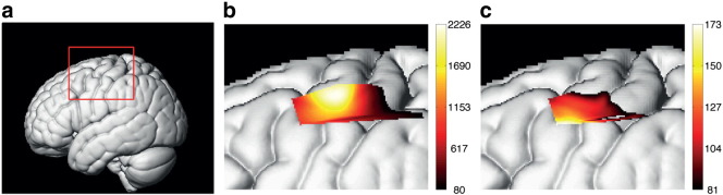
Cortical activation during motor tasks detected using oxy-hemoglobin (HbO) responses. (a) Left lateral view of volume rendered brain with bounding box showing region displayed on other two panels. (b) Main effects of motor execution task, and (c) main effects of motor imagery task. A conventional SPM analysis was applied to fNIRS data, and the resultant F-statistic maps were thresholded at a voxel level of p < 0.000001 (corrected). Results show that SMA is significantly activated during both motor execution and imagery tasks, whereas M1 was only activated during motor execution. Two regions of interest for the DCM analysis were selected using the local maxima of the F-statistics closest to M1 and lateral SMA.

DCM analysis

DCM was then fitted to the optical density signal averaged across trials. Bayesian model selection compared DCM models which differed in spatial extent of hemodynamic source, regions receiving task input, and connections modulated by motor imagery (Fig. 5). Family level inference indicated that the models with spatially distributed hemodynamic source outperformed the models with point source. Moreover, together with Bayesian inference at the model level, the best model structure was model 9 in which task input could affect regional activity in both SMA and M1, and motor imagery modulated both extrinsic and intrinsic connections.

Fig. 5.

Results of Bayesian model comparison. Family level inference indicated that models with spatially distributed hemodynamic source outperformed models with point sources. Moreover, together with Bayesian inference at the model level, the best model structure was model 9 in which task input could affect regional activity in both supplementary motor area (SMA) and primary motor cortex (M1), and motor imagery could modulate both the extrinsic and intrinsic connections.

The posterior mean DCM parameters for the best model are

$$\begin{array}{l}A=\left[\begin{array}{cc}\hfill -0.16\hfill & \hfill -0.49\hfill \\ \hfill -0.02\hfill & \hfill -0.33\hfill \end{array}\right],B^2=\left[\begin{array}{cc}\hfill -0.02\hfill & \hfill -0.77\hfill \\ \hfill 0.33\hfill & \hfill -1.31\hfill \end{array}\right],C=\left[\begin{array}{cc}\hfill 0.08\hfill & \hfill 0\hfill \\ \hfill 0.06\hfill & \hfill 0\hfill \end{array}\right]\\ \left[\begin{array}{cccccc}\hfill {\kappa }_1\hfill & \hfill {\gamma }_1\hfill & \hfill {\tau }_1\hfill & \hfill {\tau }_{1,v}\hfill & \hfill d_{1,\mathit{max}}\hfill & \hfill {\overline{\omega }}_H\hfill \\ \hfill {\kappa }_2\hfill & \hfill {\gamma }_2\hfill & \hfill {\tau }_2\hfill & \hfill {\tau }_{2,v}\hfill & \hfill d_{2,\mathit{max}}\hfill & \hfill {\overline{\omega }}_Q\hfill \end{array}\right]=\left[\begin{array}{cccccc}\hfill 0.69\hfill & \hfill 0.28\hfill & \hfill 2.11\hfill & \hfill 4.12\hfill & \hfill 4.26\hfill & \hfill 0.72\hfill \\ \hfill 0.63\hfill & \hfill 0.34\hfill & \hfill 1.97\hfill & \hfill 0.92\hfill & \hfill 3.88\hfill & \hfill 0.59\hfill \end{array}\right]\text{,}\end{array}$$

where A_i,j represents the connectivity from region j to region i in the absence of experimental input; B_i,j^k represents the change in connectivity from region j to region i induced by kth input; and C_i,k represents the influence of input on region i. The units of connections are the rates (Hz) of neural population changes. In other words, in models based upon differential equations, effective connectivity plays the role of a rate constant; where a strong influence implies a fast response. The posterior mean of estimated hemodynamic and optics parameters is within the range of values reported from the literature (Buxton et al., 2004; Huppert et al., 2009; Gagnon et al., 2012). Among estimated parameters, cortical fraction of HbO averaged across the channels $\left({\overline{\omega }}_H=0.72\right)$ was higher than that of HbR $\left({\overline{\omega }}_Q=0.59\right)$. This result suggests that the remaining 28% and 41% of the signal for HbO and HbR arise from extracerebral regions, including pial vasculature and skin, where oxygenation changes occur following brain activation. While ${\overline{\omega }}_Q$ was slightly higher than the values estimated in Gagnon et al. (2012), this discrepancy may be caused by differences in anatomical vasculature, channel position, or experimental protocol.

We selected M1 and SMA for source region 1 and source region 2, task for the first input, and motor imagery for the second input. So, as an example of analysis results, B_1,2² indicates that connectivity strength from SMA to M1 was reduced by motor imagery (− 0.77). This is entirely consistent with previous fMRI activation studies of this paradigm – and the notion that imagined movement calls on the same sensorimotor schemata here as executed movements – but gated at the level of the motor cortex. More details about the estimate of DCM parameters, including posterior variance, are shown in Fig. 6.

Fig. 6.

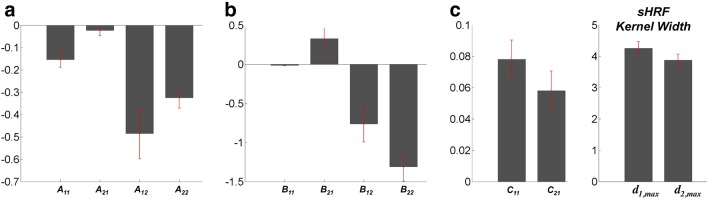
Estimates of DCM parameters, including neurodynamic and hemodynamic effects. Magnitude of bar graph indicates posterior mean of each parameter, and the red error bar indicates the standard deviation (square root of posterior variance) for model 9.

Fig. 7 shows the parameter estimates as a network model. The results indicate that while all motor stimuli positively affect the regional activity in M1, motor imagery negatively modulates the connection from SMA to M1, resulting in the suppressive influence of SMA on M1. Quantitatively, the strength of connectivity from SMA to M1, − 0.49 is significantly reduced by motor imagery, − 0.77. This suppressive influence causes reduced activity in M1 during motor imagery. Interestingly, we also found that motor imagery positively modulates the connection from M1 to SMA.

Fig. 7.

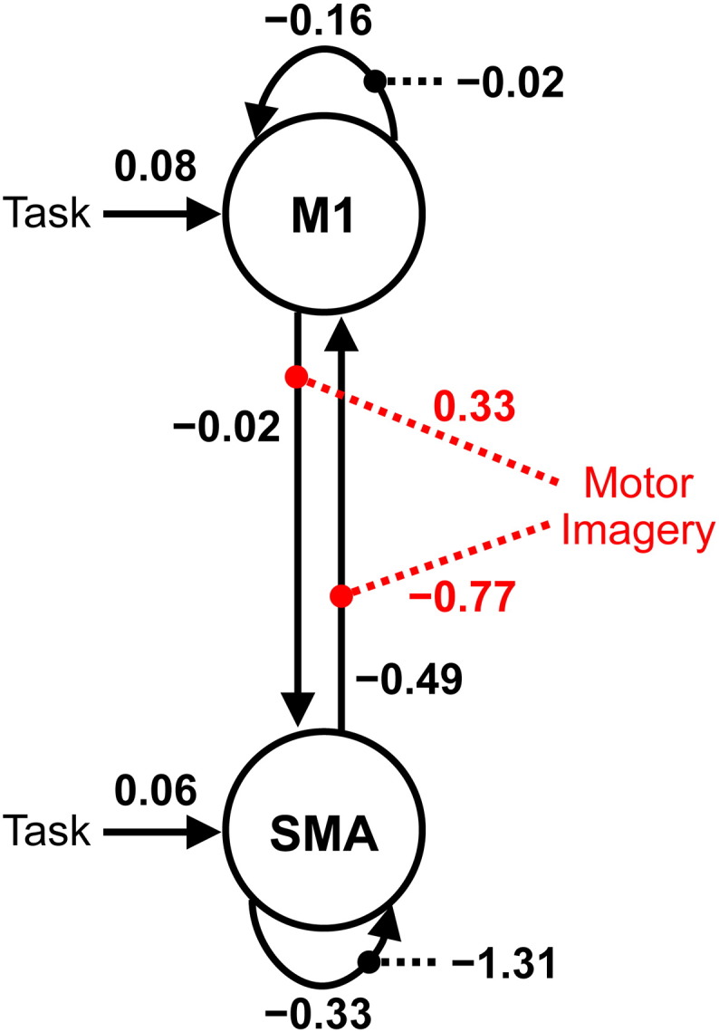
Model with estimated parameters of effective connectivity. The units of connections are the rates (Hz) of neural population changes. Black and red dotted lines indicate intrinsic and extrinsic connections modulated by motor imagery, respectively. The results indicate that while all motor stimuli positively affect the regional activity in primary motor cortex (M1), motor imagery negatively modulates connection from supplementary motor area (SMA) to M1, resulting in the suppressive influence of SMA on M1. These results are consistent with the findings of previous fMRI studies (Kasess et al., 2008; Gerardin et al., 2000).

As an example of the accuracy of DCM model fits, Fig. 8 shows the predicted and measured optical density signals. Note that our DCM models comprise two neuronal sources, including M1 and SMA, whose activities each generate optical density changes in all eight channels using the forward model in Eq. (13). To compare model fit to the channel measurements, we selected channels 2, 5, and channels 3, 4, whose sensitivities to M1 and SMA are highest among eight channels, respectively. DCM produces similar traces to the actual fNIRS data at both wavelengths 760 nm and 850 nm.

Fig. 8.

DCM fit to optical signal measured during motor execution and motor imagery. Black and blue plots indicate average optical density changes measured at wavelengths 760 nm and 850 nm, respectively. Red plots indicate the corresponding estimates from DCM model 9. To compare model fit to the measurements, we selected channels 2, 5, and channels 3, 4, whose sensitivities to M1 and SMA were highest among eight channels, respectively. DCM produces similar traces to the fNIRS data at both wavelengths. The solid black line indicates the empirical task periods (5 s), including motor execution and motor imagery.

Estimated neural responses shown in Fig. 9 show that during motor imagery, neural activity in M1 is significantly reduced, while neural activity in SMA is relatively consistent, compared with activity during motor execution. These results correspond to the findings of previous fMRI studies which have shown that M1 is more active during motor execution, while lateral SMA is more involved in motor imagery (Kasess et al., 2008; Gerardin et al., 2000).

Fig. 9.

Estimated neural responses (z). During motor imagery, neural activity in primary motor cortex (M1) is significantly reduced, while neural activity in supplementary motor area (SMA) is relatively consistent, compared with activity during motor execution. The solid black line indicates the task period (5 s).

Discussion

In this paper, we have introduced DCM for fNIRS. The generative model of fNIRS data is created by linking the fNIRS optics equation to the hemodynamic and neurodynamic equations. DCM parameters are estimated using the same Bayesian scheme which is used for dynamic causal modelling of other imaging modalities. Bayesian inference at the family and model levels then allows one to test specific hypotheses about functional brain architectures and select a model structure which explains the fNIRS data best.

Using fNIRS data whose protocol was similar to that of recent fMRI studies, we have demonstrated the validity of estimates of effective connectivity in this context. Specifically, by applying DCM to experimental data acquired during motor imagery and motor execution, we showed that the best-performing model comprised regions of SMA and M1 driven by task input, and both extrinsic and intrinsic connections are modulated by motor imagery. The corresponding estimates of DCM parameters indicated that reduced activity in M1 during motor imagery can be explained by the suppression of M1 sensitivity to extrinsic projections from SMA. These results suggest that the proposed method enables one to infer directed interactions in the brain mediated by neuronal dynamics from optical density changes.

In the following, we discuss potential extensions to the current DCM for fNIRS. One extension would be to parameterize the sensitivity matrix so that the optimal locations of hemodynamic sources are estimated from the data. Currently, we have used a fixed hemodynamic source location as identified using a prior general linear model analysis. However, because the spatial location of neuronal activation may be slightly different from hemoglobin changes, it may be appropriate to specify the location of neuronal sources as free parameters with informed priors. Motivated by the lead field parameterization in DCM for EEG and MEG (Kiebel et al., 2006), we can make the sensitivity matrix a function of three location parameters, S(θ) where θ = (x^pos, x^pos, z^pos). The expectation of the location prior can be given by an activated voxel location at the cortical level. Then, hemodynamic source locations can be estimated simultaneously with other DCM parameters using Bayesian inversion. Furthermore, we can test the hypothesis that neuronal and hemodynamic responses are spatially dislocated by comparing models with and without free location parameters.

A further area of research concerns the development of the hemodynamic equation. In the proposed scheme, the hemodynamic component is based on the extended Balloon model (Buxton et al., 2004). This model can describe transient characteristics of blood flow and blood volume, particularly in the return-to-baseline stages of the response, using viscoelastic time constant τ_j,v. As shown in Fig. 8, an undershoot of optical responses was observed during post-stimulus. In the M1 source, significantly suppressed neuronal activity and longer viscoelastic time constants were estimated. These estimates lead to decreased blood flow and delayed blood volume recovery, which increases HbR, and then leads to an undershoot of optical responses in the corresponding channels, 2, 4, and 5. This result is supported by simultaneous fMRI and electrophysical recording studies, demonstrating the correlation between negative fMRI response and decreased neuronal activity (Shmuel et al., 2006). However, our model did not fit the post-stimulus undershoot of optical response in channel 3 (Fig. 8(b)). Note that sensitivity of channel 3 to the SMA source was approximately 9 times higher than the sensitivity to the M1 source: S_3,SMA/(S_3,M1 + S_3,SMA) = 0.89. Therefore, less suppression of neuronal activity during motor execution or shorter viscoelastic time constants in SMA would cause less undershoot of estimated optical response in channel 3. More sophisticated neurodynamic (Marreiros et al., 2008; Kumar and Penny, 2014), vascular (Kong et al., 2004; Boas et al., 2008), and hemodynamic (Zheng et al., 2002; Havlicek et al., 2014) models may allow the transient hemodynamic response, such as post-stimulus undershoot, to be better fitted from fNIRS data, and to be explained by either neuronal or hemodynamic effects or both.

In this paper we have modeled each hemodynamic source as either a point process or a spatially distributed process at a specified anatomical location. In the latter case, the spatial point spread function is modeled as a Gaussian kernel whose width is estimated from data. However, this implies that the hemodynamic response is a simple low-pass spatial filter of neuronal activity. Instead, intrinsic spatiotemporal hemodynamics could be specified using differential equations specifying such spatio-temporal dynamics as a function of position on the cortical surface (Aquino et al., 2012, 2014).

Finally, we will extend the neurodynamic model to include both excitatory and inhibitory states in each region. Current DCM for fNIRS is based on a model which describes the neurodynamics with one state in each region (see Eq. (1)). By adopting a two-state neurodynamic model (Marreiros et al., 2008), we can not only model both intrinsic and excitatory activities within intrinsic coupling, but also relax the priors used to ensure stability in the one-state model. The high temporal resolution of fNIRS should in principle allow fNIRS data to support these much richer dynamical models.

A current limitation of DCM for fNIRS is that model fitting is computationally demanding, compared with functional connectivity and Granger causality analyses. For the analysis of our fNIRS data, parameter estimation in the fully connected network model comprising two regions took approximately 6 min (for point hemodynamic sources), and 18 min (for spatially distributed hemodynamic sources) on a desktop PC running Windows 7 (64 bit) with an Intel Xeon W3570 (3.2 GHz) and 12 GB RAM. The VL optimization procedure required 20 iterations and 49 iterations until it converged, respectively.

In this study, we focused on the development and description of a novel method to estimate effective connectivity from fNIRS data. We therefore showed an illustrative analysis using fNIRS data from a single subject. In a subsequent paper, we will focus on analysis of fNIRS data from a group of subjects (including random effects model comparison Stephan et al., 2009), and show clinical applications of DCM-fNIRS in patients in low awareness states.

The proposed methods are implemented in Matlab code and will be available freely in the next beta version of SPM software (http://fil.ion.ucl.ac.uk/spm).

References

- Aquino K.M., Schira M.M., Robinson P.A., Drysdale P.M., Breakspear M. Hemodynamic traveling waves in human visual cortex. PLoS Comput. Biol. 2012;8(3):e1002435. doi: 10.1371/journal.pcbi.1002435. [DOI] [PMC free article] [PubMed] [Google Scholar]
- Aquino K.M., Robinson P.A., Drysdale P.M. Spatiotemporal hemodynamic response functions derived from physiology. J. Theor. Biol. 2014;347:118–136. doi: 10.1016/j.jtbi.2013.12.027. [DOI] [PubMed] [Google Scholar]
- Arridge S.R. Optical tomography in medical imaging. Inverse Prob. 1999;15:R41–R93. [Google Scholar]
- Bishop C.M. vol. 1. Springer; New York: 2006. (Pattern Recognition and Machine Learning). [Google Scholar]
- Boas D.A., Culver J.P., Stott J.J., Dunn A.K. Three dimensional Monte Carlo code for photon migration through complex heterogeneous media including the adult human head. Opt. Express. 2002;10:159–170. doi: 10.1364/oe.10.000159. [DOI] [PubMed] [Google Scholar]
- Boas D.A., Strangman G., Culver J.P., Hoge R.D., Jasdzewski G., Poldrack R.A., Rosen B.R., Mandeville J.B. Can the cerebral metabolic rate of oxygen be estimated with near-infrared spectroscopy? Phys. Med. Biol. 2003;48(15):2405–2418. doi: 10.1088/0031-9155/48/15/311. [DOI] [PubMed] [Google Scholar]
- Boas D.A., Dale A.M., Franceschini M.A. Diffuse optical imaging of brain activation: approaches to optimizing image sensitivity, resolution, and accuracy. NeuroImage. 2004;23:S275–S288. doi: 10.1016/j.neuroimage.2004.07.011. [DOI] [PubMed] [Google Scholar]
- Boas D.A., Jones S.R., Devor A., Huppert T.J., Dale A.M. A vascular anatomical network model of the spatio-temporal response to brain activation. NeuroImage. 2008;40(3):1116–1129. doi: 10.1016/j.neuroimage.2007.12.061. [DOI] [PMC free article] [PubMed] [Google Scholar]
- Buxton R.B. Dynamic models of BOLD contrast. NeuroImage. 2012;62(2):953–961. doi: 10.1016/j.neuroimage.2012.01.012. [DOI] [PMC free article] [PubMed] [Google Scholar]
- Buxton R., Wong E., Frank L. Dynamics of blood flow and oxygenation changes during brain activation: the balloon model. Magn. Reson. Med. 1998;39:855–864. doi: 10.1002/mrm.1910390602. [DOI] [PubMed] [Google Scholar]
- Buxton R.B., Uludag K., Dubowitz D.J., Liu T.T. Modeling the hemodynamic response to brain activation. NeuroImage. 2004;23:220–233. doi: 10.1016/j.neuroimage.2004.07.013. [DOI] [PubMed] [Google Scholar]
- Cooper R.J., Caffini M., Dubb J., Fang Q., Custo A., Tsuzuki D., Fischl B., Wells W., III, Dan I., Boas D.A. Validating atlas-guided DOT: a comparison of diffuse optical tomography informed by atlas and subject-specific anatomies. NeuroImage. 2012;62:1999–2006. doi: 10.1016/j.neuroimage.2012.05.031. [DOI] [PMC free article] [PubMed] [Google Scholar]
- Cui X., Bray S., Reiss A.L. Functional near infrared spectroscopy (NIRS) signal improvement based on negative correlation between oxygenated and deoxygenated hemoglobin dynamics. NeuroImage. 2010;49:3039–3046. doi: 10.1016/j.neuroimage.2009.11.050. [DOI] [PMC free article] [PubMed] [Google Scholar]
- Daunizeau J., Friston K.J., Kiebel S.J. Variational Bayesian identification and prediction of stochastic nonlinear dynamic causal models. Physica D. 2009;238(21):2089–2118. doi: 10.1016/j.physd.2009.08.002. [DOI] [PMC free article] [PubMed] [Google Scholar]
- Daunizeau J., Kiebel S.J., Friston K.J. Dynamic causal modelling of distributed electromagnetic responses. NeuroImage. 2009;47(2):590–601. doi: 10.1016/j.neuroimage.2009.04.062. [DOI] [PMC free article] [PubMed] [Google Scholar]
- Dehaes M., Gagnon L., Lesage F., Pélégrini-Issac M., Vignaud A., Valabregue R., Grebe R., Wallois F., Benali H. Quantitative investigation of the effect of the extra-cerebral vasculature in diffuse optical imaging: a simulation study. Biomed. Opt. Express. 2011;2(3):680–695. doi: 10.1364/BOE.2.000680. [DOI] [PMC free article] [PubMed] [Google Scholar]
- Dehghani H., Eames M.E., Yalavarthy P.K., Davis S.C., Srinivasan S., Carpenter C.M., Pogue B.W., Paulsen K.D. Near infrared optical tomography using NIRFAST: algorithm for numerical model and image reconstruction. Commun. Numer. Methods Eng. 2009;25:711–732. doi: 10.1002/cnm.1162. [DOI] [PMC free article] [PubMed] [Google Scholar]
- Delpy D.T., Cope M., Van der Zee P., Arridge S., Wray S., Wyatt J. Estimation of optical pathlength through tissue from direct time of flight measurement. Phys. Med. Biol. 1988;33(12):1433–1442. doi: 10.1088/0031-9155/33/12/008. [DOI] [PubMed] [Google Scholar]
- Dubeau S., Havlicek M., Beaumont E., Ferland G., Lesage F., Pouliot P. Neurovascular deconvolution of optical signals as a proxy for the true neuronal inputs. J. Neurosci. Methods. 2012;210(2):247–258. doi: 10.1016/j.jneumeth.2012.07.008. [DOI] [PubMed] [Google Scholar]
- Eggebrecht A.T., White B.R., Ferradal S.L., Chen C., Zhan Y., Snyder A.Z., Dehghani H., Culver J.P. A quantitative spatial comparison of high-density diffuse optical tomography and fMRI cortical mapping. NeuroImage. 2012;61:1120–1128. doi: 10.1016/j.neuroimage.2012.01.124. [DOI] [PMC free article] [PubMed] [Google Scholar]
- Eggebrecht A.T., Ferradal S.L., Robichaux-Viehoever A., Hassanpour M.S., Dehghani H., Snyder A.Z., Hershey T., Culver J.P. Mapping distributed brain function and networks with diffuse optical tomography. Nat. Photonics. 2014;8:448–454. doi: 10.1038/nphoton.2014.107. [DOI] [PMC free article] [PubMed] [Google Scholar]
- Fang Q. Mesh-based Monte Carlo method using fast ray-tracing in Plücker coordinates. Biomed. Opt. Express. 2010;1:165–175. doi: 10.1364/BOE.1.000165. [DOI] [PMC free article] [PubMed] [Google Scholar]
- Fang Q., Boas D.A. IEEE International Symposium on Biomedical Imaging 2009. IEEE; 2009. Tetrahedral mesh generation from volumetric binary and grayscale images; pp. 1142–1145. [Google Scholar]
- Ferradal S.L., Eggebrecht A.T., Hassanpour M., Snyder A.Z., Culver J.P. Atlas-based head modeling and spatial normalization for high-density diffuse optical tomography: in vivo validation against fMRI. NeuroImage. 2014;85:117–126. doi: 10.1016/j.neuroimage.2013.03.069. [DOI] [PMC free article] [PubMed] [Google Scholar]
- Ferrari M., Quaresima V. A brief review on the history of human functional near-infrared spectroscopy (fNIRS) development and fields of application. NeuroImage. 2012;63(2):921–935. doi: 10.1016/j.neuroimage.2012.03.049. [DOI] [PubMed] [Google Scholar]
- Fox P.T., Raichle M.E. Focal physiological uncoupling of cerebral blood flow and oxidative metabolism during somatosensory stimulation in human subjects. Proc. Natl. Acad. Sci. U. S. A. 1986;83(4):1140–1144. doi: 10.1073/pnas.83.4.1140. [DOI] [PMC free article] [PubMed] [Google Scholar]
- Friston K.J., Holmes A.P., Worsley K.J., Poline J.-B., Frith C.D., Frackowiak R.S.J. Statistical parametric maps in functional imaging: a general linear approach. Hum. Brain Mapp. 1995;2:189–210. [Google Scholar]
- Friston K.J., Mechelli A., Turner R., Price C.J. Nonlinear responses in fMRI: the Balloon model, Volterra kernels, and other hemodynamics. NeuroImage. 2000;12(4):466–477. doi: 10.1006/nimg.2000.0630. [DOI] [PubMed] [Google Scholar]
- Friston K.J., Harrison L.M., Penny W.D. Dynamic causal modelling. NeuroImage. 2003;19(4):1273–1302. doi: 10.1016/s1053-8119(03)00202-7. [DOI] [PubMed] [Google Scholar]
- Friston K.J., Mattout J., Trujillo-Barreto N., Ashburner J., Penny W.D. Variational free energy and the Laplace approximation. NeuroImage. 2007;34(1):220–234. doi: 10.1016/j.neuroimage.2006.08.035. [DOI] [PubMed] [Google Scholar]
- Friston K.J., Kahan J., Biswal B., Razi A. A DCM for resting state fMRI. NeuroImage. 2014;94:396–407. doi: 10.1016/j.neuroimage.2013.12.009. [DOI] [PMC free article] [PubMed] [Google Scholar]
- Gagnon L., Perdue K., Greve D.N., Goldenholz D., Kaskhedikar G., Boas D.A. Improved recovery of the hemodynamic response in diffuse optical imaging using short optode separations and state-space modeling. NeuroImage. 2011;56(3):1362–1371. doi: 10.1016/j.neuroimage.2011.03.001. [DOI] [PMC free article] [PubMed] [Google Scholar]
- Gagnon L., Yücel M.A., Dehaes M., Cooper R.J., Perdue K.L., Selb J., Huppert T.J., Hoge R.D., Boas D.A. Quantification of the cortical contribution to the NIRS signal over the motor cortex using concurrent NIRS-fMRI measurements. NeuroImage. 2012;59(4):3933–3940. doi: 10.1016/j.neuroimage.2011.10.054. [DOI] [PMC free article] [PubMed] [Google Scholar]
- Gagnon L., Yücel M.A., Boas D.A., Cooper R.J. Further improvement in reducing superficial contamination in NIRS using double short separation measurements. NeuroImage. 2014;85:127–135. doi: 10.1016/j.neuroimage.2013.01.073. [DOI] [PMC free article] [PubMed] [Google Scholar]
- Gerardin E., Sirigu A., Lehéricy S., Poline J.-B., Gaymard B., Marsault C., Agid Y., Le Bihan D. Partially overlapping neural networks for real and imagined hand movements. Cereb. Cortex. 2000;10:1093–1104. doi: 10.1093/cercor/10.11.1093. [DOI] [PubMed] [Google Scholar]
- Goodwin J.R., Gaudet C.R., Berger A.J. Short-channel functional near-infrared spectroscopy regressions improve when source–detector separation is reduced. Neurophotonics. 2014;1(1):015002. doi: 10.1117/1.NPh.1.1.015002. [DOI] [PMC free article] [PubMed] [Google Scholar]
- Grubb R.L.J., Raichle M.E., Eichling J.O., Ter-Pogossian M.M. The effects of changes in PaCO2 on cerebral blood volume, blood flow, and vascular mean transit time. Stroke. 1974;5(5):630–639. doi: 10.1161/01.str.5.5.630. [DOI] [PubMed] [Google Scholar]
- Hanakawa T., Immisch I., Toma K., Dimyan M.A., Van Gelderen P., Hallett M. Functional properties of brain areas associated with motor execution and imagery. J. Neurophysiol. 2003;89:989–1002. doi: 10.1152/jn.00132.2002. [DOI] [PubMed] [Google Scholar]
- Havlicek M., Roebroeck A., Friston K., Gardumi A., Uludag K. OHBM Annual Meeting, Hamburg, Poster 1839. 2014. New physiological framework for dynamic causal modelling of fMRI data. [Google Scholar]
- Heiskala J., Pollari M., Metsńranta M., Grant P.E., Nissilń I. Probabilistic atlas can improve reconstruction from optical imaging of the neonatal brain. Opt. Express. 2009;17:14977–14992. doi: 10.1364/oe.17.014977. [DOI] [PubMed] [Google Scholar]
- Highton D., Elwell C., Smith M. Noninvasive cerebral oximetry: is there light at the end of the tunnel? Curr. Opin. Anaesthesiol. 2010;23(5):576–581. doi: 10.1097/aco.0b013e32833e1536. [DOI] [PubMed] [Google Scholar]
- Holmes C.J., Hoge R., Collins L., Woods R., Toga A.W., Evans A.C. Enhancement of MR images using registration for signal averaging. J. Comput. Assist. Tomogr. 1998;22:324–333. doi: 10.1097/00004728-199803000-00032. [DOI] [PubMed] [Google Scholar]
- Homae F., Watanabe H., Otobe T., Nakano T., Go T., Konishi Y., Taga G. Development of global cortical networks in early infancy. J. Neurosci. 2010;30(14):4877–4882. doi: 10.1523/JNEUROSCI.5618-09.2010. [DOI] [PMC free article] [PubMed] [Google Scholar]
- Hoshi Y. Functional near-infrared spectroscopy: current status and future prospects. J. Biomed. Opt. 2007;12(6):062106. doi: 10.1117/1.2804911. [DOI] [PubMed] [Google Scholar]
- Huppert T.J., Allen M.S., Diamond S.G., Boas D.A. Estimating cerebral oxygen metabolism from fMRI with a dynamic multicompartment Windkessel model. Hum. Brain Mapp. 2009;30(5):1548–1567. doi: 10.1002/hbm.20628. [DOI] [PMC free article] [PubMed] [Google Scholar]
- Im C.-H., Jung Y.-J., Lee S., Koh D., Kim D.-W., Kim B.-M. Estimation of directional coupling between cortical areas using Near-Infrared Spectroscopy (NIRS) Opt. Express. 2010;18:5730–5739. doi: 10.1364/OE.18.005730. [DOI] [PubMed] [Google Scholar]
- Jin T., Kim S.-G. Cortical layer-dependent dynamic blood oxygenation, cerebral blood flow and cerebral blood volume responses during visual stimulation. NeuroImage. 2008;43(1):1–9. doi: 10.1016/j.neuroimage.2008.06.029. [DOI] [PMC free article] [PubMed] [Google Scholar]
- Jobsis F.F. Noninvasive, infrared monitoring of cerebral and myocardial oxygen sufficiency and circulatory parameters. Science. 1977;198(4323):1264–1267. doi: 10.1126/science.929199. [DOI] [PubMed] [Google Scholar]
- Kasess C.H., Windischberger C., Cunnington R., Lanzenberger R., Pezawas L., Moser E. The suppressive influence of SMA on M1 in motor imagery revealed by fMRI and dynamic causal modeling. NeuroImage. 2008;40:828–837. doi: 10.1016/j.neuroimage.2007.11.040. [DOI] [PubMed] [Google Scholar]
- Kiebel S.J., David O., Friston K.J. Dynamic causal modelling of evoked responses in EEG/MEG with lead field parameterization. NeuroImage. 2006;30(4):1273–1284. doi: 10.1016/j.neuroimage.2005.12.055. [DOI] [PubMed] [Google Scholar]
- Kirilina E., Jelzow A., Heine A., Niessing M., Wabnitz H., Brühl R., Ittermann B., Jacobs A.M., Tachtsidis I. The physiological origin of task-evoked systemic artefacts in functional near infrared spectroscopy. NeuroImage. 2012;61(1):70–81. doi: 10.1016/j.neuroimage.2012.02.074. [DOI] [PMC free article] [PubMed] [Google Scholar]
- Kong Y., Zheng Y., Johnston D., Martindale J., Jones M., Billings S., Mayhew J. A model of the dynamic relationship between blood flow and volume changes during brain activation. J. Cereb. Blood Flow Metab. 2004;24(12):1382–1392. doi: 10.1097/01.WCB.0000141500.74439.53. [DOI] [PubMed] [Google Scholar]
- Kumar S., Penny W. Estimating neural response functions from fMRI. Front. Neuroinform. 2014;8:48. doi: 10.3389/fninf.2014.00048. [DOI] [PMC free article] [PubMed] [Google Scholar]
- Liebert A., Wabnitz H., Steinbrink J., Obrig H., Möller M., Macdonald R., Villringer A., Rinneberg H. Time-resolved multidistance near-infrared spectroscopy of the adult head: intracerebral and extracerebral absorption changes from moments of distribution of times of flight of photons. Appl. Opt. 2004;43(15):3037–3047. doi: 10.1364/ao.43.003037. [DOI] [PubMed] [Google Scholar]
- Lloyd-Fox S., Blasi A., Elwell C. Illuminating the developing brain: the past, present and future of functional near infrared spectroscopy. Neurosci. Biobehav. Rev. 2010;34(3):269–284. doi: 10.1016/j.neubiorev.2009.07.008. [DOI] [PubMed] [Google Scholar]
- Lu C.-M., Zhang Y.-J., Biswal B.B., Zang Y.-F., Peng D.-L., Zhu C.-Z. Use of fNIRS to assess resting state functional connectivity. J. Neurosci. Methods. 2010;186(2):242–249. doi: 10.1016/j.jneumeth.2009.11.010. [DOI] [PubMed] [Google Scholar]
- Luppino G., Matelli M., Camarda R., Rizzolatti G. Corticocortical connections of area F3 (SMA-proper) and area F6 (pre-SMA) in the macaque monkey. J. Comp. Neurol. 1993;338(1):114–140. doi: 10.1002/cne.903380109. [DOI] [PubMed] [Google Scholar]
- Marreiros A.C., Kiebel S.J., Friston K.J. Dynamic causal modelling for fMRI: a two-state model. NeuroImage. 2008;39(1):269–278. doi: 10.1016/j.neuroimage.2007.08.019. [DOI] [PubMed] [Google Scholar]
- Mesquita R.C., Franceschini M.A., Boas D.A. Resting state functional connectivity of the whole head with near-infrared spectroscopy. Biomed. Opt. Express. 2010;1:324–336. doi: 10.1364/BOE.1.000324. [DOI] [PMC free article] [PubMed] [Google Scholar]
- Minati L., Kress I.U., Visani E., Medford N., Critchley H.D. Intra- and extra-cranial effects of transient blood pressure changes on brain near-infrared spectroscopy (NIRS) measurements. J. Neurosci. Methods. 2011;197(2):283–288. doi: 10.1016/j.jneumeth.2011.02.029. [DOI] [PMC free article] [PubMed] [Google Scholar]
- Moran R.J., Kiebel S.J., Stephan K.E., Reilly R.B., Daunizeau J., Friston K.J. A neural mass model of spectral responses in electrophysiology. NeuroImage. Sep 2007;37(3):706–720. doi: 10.1016/j.neuroimage.2007.05.032. [DOI] [PMC free article] [PubMed] [Google Scholar]
- Muakkassa K.F., Strick P.L. Frontal lobe inputs to primate motor cortex: evidence for four somatotopically organized ‘premotor’ areas. Brain Res. 1979;177(1):176–182. doi: 10.1016/0006-8993(79)90928-4. [DOI] [PubMed] [Google Scholar]
- Obrig H. NIRS in clinical neurology — a ‘promising’ tool? NeuroImage. 2014;85:535–546. doi: 10.1016/j.neuroimage.2013.03.045. [DOI] [PubMed] [Google Scholar]
- Obrig H., Neufang M., Wenzel R., Kohl M., Steinbrink J., Einhäupl K., Villringer A. Spontaneous low frequency oscillations of cerebral hemodynamics and metabolism in human adults. NeuroImage. 2000;12(6):623–639. doi: 10.1006/nimg.2000.0657. [DOI] [PubMed] [Google Scholar]
- Penny W.D. Comparing dynamic causal models using AIC, BIC and free energy. NeuroImage. 2012;59:319–330. doi: 10.1016/j.neuroimage.2011.07.039. [DOI] [PMC free article] [PubMed] [Google Scholar]
- Penny W., Litvak V., Fuentemilla L., Duzel E., Friston K. Dynamic Causal Models for phase coupling. J. Neurosci. Methods. 2009;183(1):19–30. doi: 10.1016/j.jneumeth.2009.06.029. [DOI] [PMC free article] [PubMed] [Google Scholar]
- Penny W.D., Stephan K.E., Daunizeau J., Rosa M.J., Friston K.J., Schofield T.M., Leff A.P. Comparing families of dynamic causal models. PLoS Comput. Biol. 2010;6(3):e1000709. doi: 10.1371/journal.pcbi.1000709. [DOI] [PMC free article] [PubMed] [Google Scholar]
- Saager R.B., Telleri N.L., Berger A.J. Two-detector Corrected Near Infrared Spectroscopy (C-NIRS) detects hemodynamic activation responses more robustly than single-detector NIRS. NeuroImage. 2011;55(4):1679–1685. doi: 10.1016/j.neuroimage.2011.01.043. [DOI] [PubMed] [Google Scholar]
- Sasai S., Homae F., Watanabe H., Taga G. Frequency-specific functional connectivity in the brain during resting state revealed by NIRS. NeuroImage. 2011;56(1):252–257. doi: 10.1016/j.neuroimage.2010.12.075. [DOI] [PubMed] [Google Scholar]
- Scholkmann F., Gerber U., Wolf M., Wolf U. End-tidal CO2: an important parameter for a correct interpretation in functional brain studies using speech tasks. NeuroImage. 2013;66:71–79. doi: 10.1016/j.neuroimage.2012.10.025. [DOI] [PubMed] [Google Scholar]
- Scholkmann F., Kleiser S., Metz A.J., Zimmermann R., Mata Pavia J., Wolf U., Wolf M. A review on continuous wave functional near-infrared spectroscopy and imaging instrumentation and methodology. NeuroImage. 2014;85:6–27. doi: 10.1016/j.neuroimage.2013.05.004. [DOI] [PubMed] [Google Scholar]
- Shmuel A., Augath M., Oeltermann A., Logothetis N.K. Negative functional MRI response correlates with decreases in neuronal activity in monkey visual area V1. Nat. Neurosci. 2006;9(4):569–577. doi: 10.1038/nn1675. [DOI] [PubMed] [Google Scholar]
- Shmuel A., Yacoub E., Chaimow D., Logothetis N.K., Ugurbil K. Spatio-temporal point-spread function of fMRI signal in human gray matter at 7 Tesla. NeuroImage. 2007;35(2):539–552. doi: 10.1016/j.neuroimage.2006.12.030. [DOI] [PMC free article] [PubMed] [Google Scholar]
- Stephan K., Weiskopf N., Drysdale P., Robinson P., Friston K. Comparing hemodynamic models with DCM. NeuroImage. 2007;38(3):387–401. doi: 10.1016/j.neuroimage.2007.07.040. [DOI] [PMC free article] [PubMed] [Google Scholar]
- Stephan K.E., Kasper L., Harrison L.M., Daunizeau J., den Ouden H.E., Breakspear M., Friston K.J. Nonlinear dynamic causal models for fMRI. NeuroImage. 2008;42:649–662. doi: 10.1016/j.neuroimage.2008.04.262. [DOI] [PMC free article] [PubMed] [Google Scholar]
- Stephan K.E., Penny W.D., Daunizeau J., Moran R.J., Friston K.J. Bayesian model selection for group studies. NeuroImage. 2009;46(4):1004–1017. doi: 10.1016/j.neuroimage.2009.03.025. [DOI] [PMC free article] [PubMed] [Google Scholar]
- Tachtsidis I., Leung T.S., Chopra A., Koh P.H., Reid C.B., Elwell C.E. Oxygen Transport to Tissue XXX. Springer; 2009. False positives in functional nearinfrared topography; pp. 307–314. [DOI] [PubMed] [Google Scholar]
- Takahashi T., Takikawa Y., Kawagoe R., Shibuya S., Iwano T., Kitazawa S. Influence of skin blood flow on near-infrared spectroscopy signals measured on the forehead during a verbal fluency task. NeuroImage. 2011;57:991–1002. doi: 10.1016/j.neuroimage.2011.05.012. [DOI] [PubMed] [Google Scholar]
- Tong Y., Lindsey K.P., deB Frederick B. Partitioning of physiological noise signals in the brain with concurrent near-infrared spectroscopy and fMRI. J. Cereb. Blood Flow Metab. 2011;31(12):2352–2362. doi: 10.1038/jcbfm.2011.100. [DOI] [PMC free article] [PubMed] [Google Scholar]
- Villringer A., Planck J., Hock C., Schleinkofer L., Dirnagl U. Near infrared spectroscopy (NIRS): a new tool to study hemodynamic changes during activation of brain function in human adults. Neurosci. Lett. 1993;154(1):101–104. doi: 10.1016/0304-3940(93)90181-j. [DOI] [PubMed] [Google Scholar]
- Wang L., Jacques S.L., Zheng L. MCML — Monte Carlo modeling of light transport in multi-layered tissues. Comput. Meth. Programs Biomed. 1995;47:131–146. doi: 10.1016/0169-2607(95)01640-f. [DOI] [PubMed] [Google Scholar]
- White B.R., Snyder A.Z., Cohen A.L., Petersen S.E., Raichle M.E., Schlaggar B.L., Culver J.P. Resting-state functional connectivity in the human brain revealed with diffuse optical tomography. NeuroImage. 2009;47(1):148–156. doi: 10.1016/j.neuroimage.2009.03.058. [DOI] [PMC free article] [PubMed] [Google Scholar]
- Wolf M., Naulaers G., van Bel F., Kleiser S., Griesen G. Review: a review of near infrared spectroscopy for term and preterm newborns. J. Near Infrared Spectrosc. 2012;20(1):43–55. [Google Scholar]
- Yacoub E., Ugurbil K., Harel N. The spatial dependence of the poststimulus undershoot as revealed by high-resolution BOLD- and CBV-weighted fMRI. J. Cereb. Blood Flow Metab. 2005;26(5):634–644. doi: 10.1038/sj.jcbfm.9600239. [DOI] [PubMed] [Google Scholar]
- Ye J.C., Tak S., Jang K.E., Jung J., Jang J. NIRS-SPM: statistical parametric mapping for near-infrared spectroscopy. NeuroImage. 2009;44:428–447. doi: 10.1016/j.neuroimage.2008.08.036. [DOI] [PubMed] [Google Scholar]
- Yuan Z. Combining independent component analysis and Granger causality to investigate brain network dynamics with fNIRS measurements. Biomed. Opt. Express. 2013;4:2629–2643. doi: 10.1364/BOE.4.002629. [DOI] [PMC free article] [PubMed] [Google Scholar]
- Yücel M.A., Huppert T.J., Boas D.A., Gagnon L. Calibrating the BOLD signal during a motor task using an extended fusion model incorporating DOT, BOLD and ASL data. NeuroImage. 2012;61(4):1268–1276. doi: 10.1016/j.neuroimage.2012.04.036. [DOI] [PMC free article] [PubMed] [Google Scholar]
- Zheng Y., Martindale J., Johnston D., Jones M., Berwick J., Mayhew J. A model of the hemodynamic response and oxygen delivery to brain. NeuroImage. 2002;16(3):617–637. doi: 10.1006/nimg.2002.1078. [DOI] [PubMed] [Google Scholar]