Abstract
Image registration has been proposed as an automatic method for recovering cardiac displacement fields from Tagged Magnetic Resonance Imaging (tMRI) sequences. Initially performed as a set of pairwise registrations, these techniques have evolved to the use of 3D+t deformation models, requiring metrics of joint image alignment (JA). However, only linear combinations of cost functions defined with respect to the first frame have been used. In this paper, we have applied k-Nearest Neighbors Graphs (kNNG) estimators of the a-entropy (Ha) to measure the joint similarity between frames, and to combine the information provided by different cardiac views in an unified metric. Experiments performed on six subjects showed a significantly higher accuracy (p < 0.05) with respect to a standard pairwise alignment (PA) approach in terms of mean positional error and variance with respect to manually placed landmarks. The developed method was used to study strains in patients with myocardial infarction, showing a consistency between strain, infarction location, and coronary occlusion. This paper also presents an interesting clinical application of graph-based metric estimators, showing their value for solving practical problems found in medical imaging.
1. Introduction
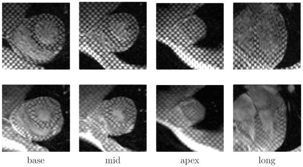
Tagged Magnetic Resonance Imaging (tMRI) is currently the reference modality for obtaining regional information on myocardial deformation. Since its introduction by Zerhouni et al. (1988) for cardiac function assessment, this technique has rapidly evolved due to advances in image acquisition, image processing, and clinical applications. Figure 1 shows an example of images of the heart obtained with tMRI. The continuous efforts of researchers to obtain a completely automatic and reliable method for recovering cardiac motion and deformation, have generated interest in this modality. Pai and Axel (2006) have presented a review of technical and clinical advances in this arena.
Figure 1.
Example of the tMRI images of the heart. From left to right: basal, medial, apical, and longitudinal planes of the left ventricle (LV). The top row corresponds to End-of-Diastole (ED) and the bottom row to End-of-Systole (ED).
The estimation of cardiac displacement fields from tMRI sequences can be formulated as an image registration problem (Chandrashekara et al., 2004a; Ledesma-Carbayo et al., 2005; Petitjean et al., 2003; Radeva et al., 1997; Shen et al., 2005), since it requires finding a point correspondence between component frames of the sequence. The application of registration techniques based on information theory (IT) (Chandrashekara et al., 2004a; Petitjean et al., 2003) is an interesting approach to cope with the non linear changes in tag intensity along the cardiac cycle. However, the evolution of transformation models towards the use of 3D + t models (Chandrashekara et al., 2004b; Ledesma-Carbayo et al., 2005) needs the definition of a metric of joint alignment to optimize simultaneously the transformation parameters. This problem can be circumvented by using a linear combination of the pairwise metrics between each phase and the reference (Chandrashekara et al., 2004b; Ledesma-Carbayo et al., 2005), but this approach still measures the image similarity with respect to the first phase and fails to exploit the temporal correlation between phases.
In this paper, we have explored an extension of IT-based registration techniques that finds the optimal transformation parameters of a 3D+t model by maximization of a metric of joint frame alignment. The main challenge in computing such metrics is the estimation of the probability density function (PDF) from a set of samples in a high-dimensional space (in our case, the sequence length). Neemuchwala et al. (2007) have recently presented estimators of α-Mutual Information MIα based on kNNG when high dimensional features are employed, and the use of histograms is not possible due to the curse of dimensionality (Bellman, 2003). Ma et al. (2007) have applied these estimators for computing deformations in a synthetic sequence of tumor images, and introduced joint similarity extensions of MIa. More recently, Leonenko et al. (2008) have presented a class of estimators of Hα based on the kth nearest-neighbor distances computed from a sample of N i.i.d. vectors with distribution f. In this article, we have extended kNNG estimators of Hα to quantify the joint alignment of multiview sequences, and applied it to tMRI sequences to recover cardiac displacement fields. For quantitative evaluation of our method, a comparison was run against the method proposed by Chandrashekara et al. (2004a) for 6 healthy subjects. Results show a significant decrease in positional error with respect to manually placed landmarks. The estimated strains were compared with those obtained by cine harmonic phase (HARP) magnetic resonance imaging as the ground truth. For assessing consistency with other modalities, we have studied two patients with myocardial infarction and compared the strain maps with the information provided by delayed-enhancement MRI of Gadolinium (deMRI) and cardiac catheterization.
2. Method
2.1. Dataset
The database used for the experiments consisted of 6 healthy subjects (3 females and 3 males between 24 and 33 years old) and 2 patients (males, 54 and 70 years old) with transmural infarction of the myocardium. For all subjects, cine MRI (cMRI), tMRI, and deMRI images were acquired in breath-hold by using a General Electric Signa CV/i, 1.5 T scanner (General Electric, Milwaukee, USA). Healthy subjects were also imaged with deMRI to have a proof of their clinical status. The values of acquisition parameters were: slice thickness 8mm, in-plane resolution 0.78mm × 0.78mm, gap between slices Omm, TR=7.99ms, TE=4.43ms, flip angle 20 degrees, and FOV=40cmx40cm. cMRI and tMRI sequences were acquired at 30 phases per cardiac cycle. tMRI images with a grid pattern of 5mm (tag spacing) were acquired by applying a Spatial Modulation of Magnetization (SPAMM) sequence. An expert clinician assessed the presence of infarction from deMRI images, and classified the 17 standard segments (Cerqueira et al., 2002) according to the transmurality of necrosis in the myocardial wall into four categories: i) 03 (healthy segment) ii) <50%, iii) 50-75% and iv) > 75%. For patients with myocardial infarction, cardiac catheterization was also performed to assess coronary occlusion.
2. 2. Deformation model
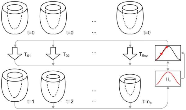
Figure 2 presents a diagram of the method of joint alignment. This figure shows that the deformation of the heart is modeled by a set of transformations defined relative to its undeformed state (ED), which simplifies the computation of metric derivatives and Lagrangian strains. The use of Lagrangian strains is more common than natural strains1 in most of current imaging techniques (US, MR, SPECT, angiography) (Sutherland et al., 2006).
Figure 2.
Cardiac motion estimation method. Transformations Toi mapping points in ED (top) to phase i (bottom) are optimized simultaneously to minimize the Hα of all phases. The inputs to the optimizer are the set of transformations T and the metric of similarity. This metric takes in turn all images of the sequence as input.
Typically, a tMRI study consists of two acquisitions performed in short axis (SA) and long axis (LA), which provide complementary information about the cardiac deformation. This results in two image sequences IsA (x, t) and ILA(x, t) of P phases, which provide the voxel intensity at spatial position × and time t. Cardiac deformation was modeled as a set of P – 1 B-Splines T (x) = {Ti (x) } i = 1 : P = 1 transformations defined on IsA(x, 0). The corresponding deformations in LA can be obtained from T (x) by composition of T (x) with the rigid transformations defining the relationship between both coordinate systems, as described in Section 2.6.
2. 3. Join t vs pairwise alignment
We explain the advantage of joint registration over pairwise registration by adopting a generative model representation of the image registration problem. A generative model for the image registration problem is obtained by expressing the log posterior probability of the deformation (B-spline parameters B) given the image sequence (Learned-Miller, 2006):
| (1) |
where N is the total number of pixels, Z is a random vector of dimension P, called a pixel stack, whose realizations are the time series of grey levels at a specified pixel location over successive image volumes in the time sequence. Each realization z ranges over the set {0, 2Q}P where Q is the number of bits quantifying image intensities. In Equation 1, p (B) is a prior on the deformation, which can be discarded by assuming a uniform probability distribution of the transformation parameters.
The conditional entropy on the right hand side of Equation 1 can be empirically estimated from Shannon entropy using (Cover and Thomas, 1991):
| (2) |
where Ni = ∑j Z:(Xj) = zi is the number of pixel locations where the associated vector Z (xj) equals grey level zi and satisfies ∑ i Ni = N.
The problem, of course, is that there are too few samples to reliably estimate the log posterior (1) due to the curse of dimensionality. Furthermore, even if one wanted to compute the log posterior, the required memory explodes as P increases (memory scales as 2P·Q). This is the justification of alternative direct methods of estimating the entropy. The MST/kNNG alphα-entropy estimators converge in probability to H Z|B) for large N and P. This is because for large N the alphα-entropy estimator converges to the alpha-entropy, by the law of large numbers, and for large P, α = (P – 1)/P ≈ 1, and the alpha-entropy is approximately equal to the Shannon entropy.
Therefore, in light of the representation (1) of the log posterior density, the PA approach corresponds to making an approximation to the entropy function defining the log posterior denotes the j-th image volume in the sequence. Such approximation to the full joint entropy is expected to be poor when a frame of the image sequence is correlated to more than just its neighboring frames, or more generally when pairwise independence of the sequence does not imply joint independence. When the decomposition of the joint distribution into pairwise successive products gives a poor approximation to the true log posterior (1), the PA method will perform poorly. For example, using standard arguments of mathematical statistics, it can be shown that in the limit as N becomes large, minimization of the pairwise entropy will give a biased estimator of the deformation parameters B, equal to the least false estimate of B (Ripley, 1996).
2.4. kNNG entropy estimator
Given a random vector Z = [Z1 … ZP] T in P, the Renyi entropy Hα of order a of Z is defined as (Renyi, 1961):
| (3) |
where f(Z1, …, Zp) is the PDF of Z.
If Z̷ {Z1, … , ZN} are the observed data (realizations of Z), a kNNG can be formed by all points and the edges with their k nearest points . An interesting property of this type of graph is the existence of a relationship between its length and the Hα of its component points:
| (4) |
where Lγ,k(Z̷) is the length of the graph defined as:
| (5) |
and γ P * (1 -α). In Equation ckNNG = (1 − α)−1 log βd,γk, where βd,γk is a known constant that depends only on d, γ, and k (Yukich, 1998).
Equation 4 suggests the following estimator of Ha(Z):
| (6) |
The demonstration of the convergence properties of kNNG estimators of entropy is out of the scope of this paper, but the reader is referred to Leonenko et al. (2008), Redmond and Yukich (1996), and Hero et al. (2003) for further reading.
There is a difference between the entropy estimation approach taken by Learned-Miller (2006) and the approach adopted in this paper. Learned-Miller assumes that intensities are independently and identically distributed (i.i.d.) both over all pixel locations and over all images inside each pixel stack. Using these two assumptions, the problem is reduced to the computation of the entropy of a scalar random variable. While the assumption of independent images inside the pixel stack Z is reasonable in the case of independent subjects, it can not be maintained in our case since we focus on temporal sequences where consecutive images are expected to be highly dependent. As a consequence, entropy must be estimated in a space of high dimensionality without any constraint about component independence in Z. The estimator in Equation 6 only assumes i.i.d realizations of Z, and therefore is suitable for our application.
A drawback of the estimator given by Equation 6 is the high computational cost of the graph construction, which hampers the parameter optimization. In the Appendix 6, we present an analytical expression for the gradient of Equation 6 reducing significantly the calculation time.
2. 5. Self matches
Equation 6 is numerically unstable when any of the distances equal to zero, i.e. in case of self matches. If Z was continuous, their realizations would cover the whole range of possible values, without any repetition. However, digital images are quantized and represented by a finite number of bits, and there exists the possibility of finding multiple occurrences of a specific value z* in Z̷. To circumvent this problem, Neemuchwala et al. (2007) added uniform noise to each realization, thus dispersing features inside a radius-limited neighborhood. Even when this approach effectively solves the problem, it might generate arbitrarily large values in the estimated PDF, and introduces a stochastic component in the cost function that could interfere with the optimization process.
In this paper, we have solved the problem of multiple occurrences by searching for nearest neighbors at a distance strictly positive, and dividing the distance by the number of occurrences oz̷ (z ) of z in Z̷. This corrects the approximation of the probabilities by using the volume of the Voronoi cell proposed by Neemuchwala and Hero (2005) in case of self matches. Even when this requires a second nearest neighbor search, the additional computational cost is negligible (Mount, 2006).
2. 6. Combination of views
A tMRI study typically contains SA and LA views of the heart that provide complimentary information about the cardiac deformation. An alternative to include both views in the registration process is a linear combination of the similarity metrics measured independently for each view (Chandrashekara et al., 2004a). However, the application of this strategy would be in conflict with the underlying ideas of this paper, which studies a manner of quantifying the alignment of a sequence as a whole. To obtain an unique metric valid for multiple views and multiple frames, each view can be considered a source of realizations of the same random vector Z. This means that pixel stacks zsa and zla taken from SA and LA are considered as realizations of the same variable Z, and can thus be mixed into a single set of samples Z̷. Under this hypothesis, Equation 3 remains unchanged for registration of multiple view sequences, integrating in this way information from different time points and views into the same unified framework.
By convention, SA has been taken as the reference space for defining the transformation. Thus, the coordinates of samples in LA must be mapped to SA to be transformed. These transformed coordinates need then to be mapped back to LA for computing the pixel stack zla. Therefore, it is necessary to know the transformations from SA to LA (Tsl) and from LA to SA (Tls). These transformations are provided by the DICOM format in the form of image origin and orientation with respect to the coordinate system of the scanner. Two generic points and in image coordinates can be expressed in world coordinates as :
| (7) |
| (8) |
When Equations 7 and 8 refer to the same physical point, we can equate the right sides and obtain the following transformations between views:
| (9) |
| (10> |
2. 7. Strain estimation
The mechanical impairment induced over time due to myocardial infarction is an important issue that can be assessed through tMRI (Axel et al., 2005). The infarcted region of diseased myocardium permanently loses its ability to contract, and this is manifested in an altered motion during the cardiac cycle. Therefore, there should be a correlation between the localization of the infarction and corresponding local strains. To study this correspondence, strain was computed from the recovered displacements fields to discriminate between active healthy myocardium and passively moving infarcted tissue.
The set of transformations T allows to compute the displacement field u (x, t) as a function of position x at ED and time t. Since the assumption of small deformations is too strong for cardiac deformations, the Green strain tensor cannot be applied, and the Green-Lagrange strain tensor must be used instead. The Green-Lagrange strain tensor is defined as (Belytschko et al., 2001)
| (11) |
Diagonal elements Eii of E are normal strains, i.e. strains along each direction in the rectangular coordinate system. Given the geometry of the heart, it is preferable to use a local coordinate system composed by radial, circumferential, and longitudinal directions (Figure 3). To estimate the epicardial surface necessary to obtain the radial direction, a manual segmentation of the SA image at ED was performed followed by the application of a variant (Schroeder et al., 1998) of the original marching cubes algorithm (Lorensen and Cline, 1987).
Figure 3.
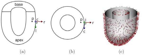
Local coordinate system used for strain analysis. Radial (r ) , circumferential (c ) , and longitudinal (1) directions for the point p are shown in the longitudinal (a) and transverse (b) views of the LV. (c) Example of radial directions obtained from the epicardial and endocardial surfaces of the LV.
The normal strain along an arbitrary direction d can be obtained from Equation 11 as (Petitjean et al., 2005):
| (12) |
Radial (Err), circumferential (Ecc), and longitudinal (Eu) normal strains can be obtained by replacing d with directions r, c, and 1, respectively.
The radial direction is defined outward and perpendicular to the epicardial surface. The circumferential direction is in the short-axis plane (perpendicular to the long axis), parallel to the epicardial surface, and counterclock wise, as viewed from the base. The longitudinal direction is obtained as the cross product of radial and circumferential directions, tangent to the epicardial surface. In this way, directions were defined to create a right-handed system.
2.8. Implementation issues
A registration-based method is composed by a transform, a metric, an interpolator, and an optimizer. In the following we describe the parameters used for each of these components in this paper. Unless the contrary is specified, the implementation of the method was performed by using the Insight Toolkit (Ibanez et al., 2008), and its component classes.
For the transformation (Section 2.2), the only parameters to specify are the spacings between control points in x, y, and z directions. We have set these spacings equal to the tag spacing (5-7mm for our dataset). A larger spacing could be insufficient to describe the deformations provided for all tags (for example, if the spacing was twice the tag spacing there would be two control points to fit three tags). On the other hand, finer grids add unnecessary degrees of freedom to the transform (there are not material points to track between two adjacent tags) and make the optimization process more difficult. This was confirmed experimentally.
Regarding the metric (Equation 6), the value of α was set to 0.9, which implies γ value of 1.0 when considering 10 frames as the length of systole. The number N of points z (i.e. #Z̷) was set to 0.2 × Nmax, Nmax being the number of points in the region of interest. The construction of the kd-tree and the nearest neighbor search was performed by using the approximate nearest neighbors (ANN) library (Mount, 2006). The use of low k-values (for example k = 1) led to misregistration of the sequences used in this paper, probably a consequence of a noisy estimation of the entropy. The use of several neighbors makes the entropy estimator more robust to noise, since the addition of the distances to the considered point in in Equation 6 tends to cancel the noise in the measurements. A number k = 20 of nearest neighbors yielded satisfying results.
For interpolation, we have used a linear interpolator. For optimization, we have used a gradient descent method with learning rate η = 1mm and a maximum number of iterations Nit = 200. The range of variation of the transformation parameters typically increases from end-systole to enddiastole, which creates optimization problems when starting from an identity transform. This type of problem may be solved by setting different scales to the parameters according to a priori information about the specific problem (Ibanez et al., 2008), but this solution led to a sequence misregistration. Therefore we reduced the range of variation of the parameters for all frames by initializing the optimizer with the result of a pairwise registration of each frame with respect to the first one (P = 2). This solution allowed us to obtain good results after joint registration, and it does not assumes any priors on the deformation.
3. Results
3.1. Entropy evolution
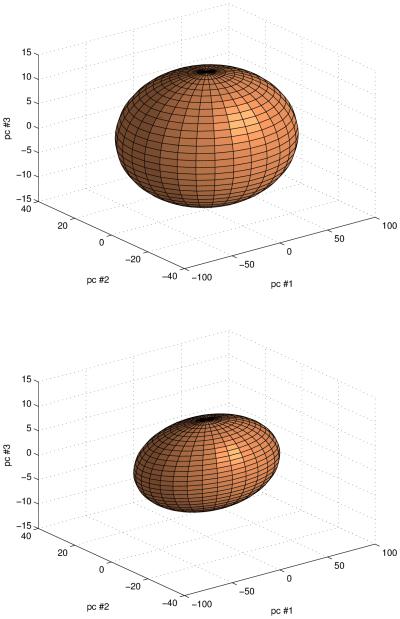
As the Hα is minimized during the registration process, the distribution of the pixel stack Z̷ after registration should be more compact with respect to the original data. To visualize this expected change in distribution, we have performed a reduction of dimensionality by applying a Principal Components Analysis (PCA) (Rao, 2002) and projected Z̷ in the subspace spanned by the first three principal directions qi=1:3. Figure 4 shows that the point distribution before registration presents a larger variance than after registration, equivalent to a state of higher entropy, as expected.
Figure 4.
Distributions of the pixel stack Z in the subspace spanned by the first three principal component directions qi=1:3. Top: before registration; bottom: after registration. Ellipsoids have semi-axis lengths equal to the standard deviation along the corresponding principal vectors q.
3. 2. Error analysis
Figure 5 presents an example of the deformation fields obtained by joint image registration, showing consistency with cardiac physiology. To compute accuracy, tag intersections were marked in the systolic phases of 6 healthy subjects by an expert clinician. Only systolic phases were marked since the images were acquired by using SPAMM, and the strong fading effect of this sequence makes difficult to identify tags beyond ES. The resulting transformations T* were used to propagate the points in ED to the remaining phases, and compare to manual measurements. Tag intersections were marked in SA at base, mid, and apex, whereas only the central plane was used in LA. On average, 24 tag intersections were tracked from ED through systole.
Figure 5.
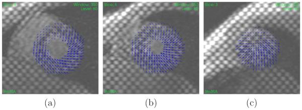
Example of displacement field at ES (relative to ED) for a healthy volunteer at (a) base, (b) mid, and (c) apex. The displacement field is plotted on the SA images at ED.
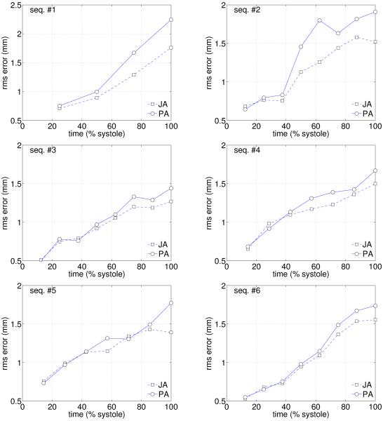
To study the differences with respect to pairwise methods, we have implemented the method proposed by Chandrashekara et al. (2004a) by using the Insight Toolkit (Ibanez et al., 2008), and compared the Mean Square Errors (MSE) along systole (Figure 6). A lower MSE was obtained for almost all cardiac phases, and a Mann-Whitney test (Altman, 1997) was performed to assess the statistical significances of these differences. The normality of the distribution was verified at level 0.05 by using a Lilliefors test (Lilliefors, 1967), and the independence of population ensured by applying each method to a different set of three sequences. Table 1 shows rejection of the null hypothesis at 5% significance level for almost all phases, meaning that the differences in MSE are statistically significant.
Figure 6.
MSE errors between manually placed landmarks at tag intersections, and propagated landmarks for six healthy volunteers. JA = joint alignment; PA = pairwise alignment.
Table 1.
p-values obtained from the Mann-Whitney test performed on the MSE errors for JA and PA methods. Results are provided for equally spaced time instants along systole. Bold values mean rejection of the null hypothesis at 5% significance level.
| time (relative to systole) | 14% | 28% | 43% | 57% | 71% | 86% | 100% |
| p-value | < 0.01 | 0.01 | < 0.01 | 0.01 | 0.01 | 0.01 | < 0.01 |
Differences in error variance (Figure 7) were also studied to assess the uniformity of the registration error across regions. It is desirable that registration accuracy be independent of the displacement magnitude, which varies across the myocardium during the cardiac cycle. The error uniformity can be measured by computing its variance. Table 2 shows the p-values obtained from a F-test (Altman, 1997) performed on the variances for each phase. As in the previous Mann-Whitney test for mean error values, each method was applied on different sequences to ensure independence.
Figure 7.
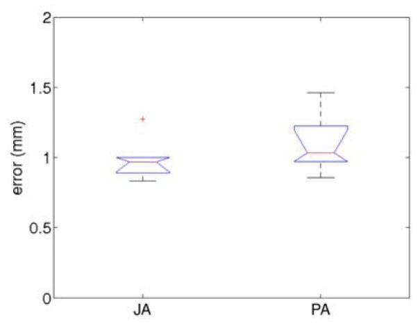
Box plots of the MSE errors showing the difference in variance between joint alignment (JA) and pairwise alignment (PA).
Table 2.
p-values obtained with a F-test performed on error variances for JA and PA methods. Bold values mean rejection of the null hypothesis of equal variances (p=0.05).
| t (relative to systole) | 14% | 28% | 43% | 67% | 71% | 86% | 100% |
| p-value | 0.29 | 0.04 | < 0.01 | < 0.01 | < 0.01 | 0.04 | 0.01 |
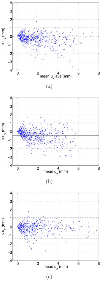
Finally, the JA method was compared to manual measurements by using Bland-Altman plots (Altman, 1997). Figure 8 shows a negligible bias, and a symmetric error distribution around it.
Figure 8.
Bland-Altman plots of displacements along x (a), y (b), and z (c) axes (Δuz). Solid and dashed lines show respflively the mean value and the 953 confidence interval of point displacements.
3. 3. Computational complexity and speed
Registration based on graphs suffers from a high computational cost that increases with the number of feature realizations. The reduction in complexity by analytical computation of the gradient of the cost function is especially advantageous when using transformations with high number of parameters. For example, if B-Splines are employed, even a coarse grid over the LV of 8x8x8 control points contains 1,536 parameters, and the gradient estimation requires 3,072 function evaluations, i.e. building 3,072 graphs. The use of analytical expressions resulted in an average computation time of 45 min for a PC with a 64 bits processor Intel Itanium at 1.5 GHz running Linux Suse 9.2. Figure 9 shows a linear increase in computation time with the number of points used to estimate Hα (the size of Z).
Figure 9.
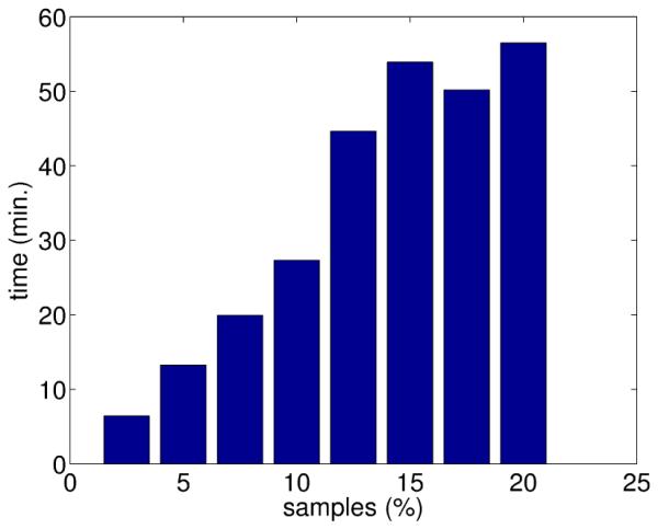
Average registration time as a function of the number of samples used for estimating Hα (expressed as percent of the number of voxels of the ROI containing the LV)
3.4. Strain in healthy subjects
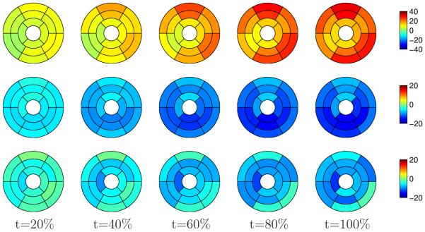
Strain analysis along systole was performed by dividing the LV into the standard 16 segments of the American Heart Association (AHA) (Cerqueira et al., 2002) (the 17th, apical segment is optional). The average and standard deviation of radial, circumferential, and longitudinal strain were computed for the 6 healthy subjects. The strain analysis was constrained to systole because of the same data acquisition issues mentioned in Section 3.2. Figure 10 shows the mean strain along systole for healthy subjects. Radial strain presented the highest variability in agreement with previous reports (Moore et al., 2000; Petitjean et al., 2004). The strain sign is consistent with the heart physiology: during systole there is a radial thickening (positive strain), and circumferential and longitudinal shortening (negative strain).
Figure 10.
Mean strain over systole for healthy subjects estimated with our method. Top row: radial strain; middle row: circumferential strain; bottom row: longitudinal. Time is expressed as percent of systole.
Our method was compared to cine harmonic phase (HARP) magnetic resonance imaging method (Osman et al., 1999) as the ground truth (Figure 11). The datasets were analyzed at the Johns Hopkins University using Diagnosoft2, a state-of-the-art software for cardiac image analysis.
Figure 11.
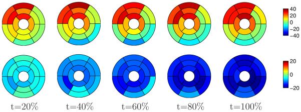
Mean strain over systole for healthy subjects estimated by using HARP. Top row: radial strain; bottom row: circumferential strain. Time is expressed as percent of systole. Longitudinal strains are not included because Diagnosoft processes short-axis images only.
3. 5. Strain in myocardial infarction
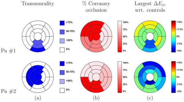
To assess consistency of the results with expected deformations in pathological cases, a strain analysis was performed on two patients with myocardial infarction. Figure 12 shows the infarction location, regions at risk, and circumferential strains for these patients. This analysis consisted in a segment- to-segment comparison of circumferential strain with respect to the normal subjects. The choice of circumferential strain for comparison is due to the small intersubject variability of healthy subjects as compared to radial and longitudinal strain. This makes easier the detection of any deviation in strain with respect to normal values. Figure 12 shows that for patient #1 the largest deviations with respect to normality are found in segments BI, MI, and AI, coinciding with the infarction location at the inferior area of the LV. Segments BA, MA, and BAS showed an increased strain on the opposite side of the infarction, which could be explained as a compensatory mechanism of healthy segments to maintain the systolic function close to normal level. In patient #2, all infarcted segments presented a lower strain with respect to the control group. Even when the lateral wall had no evidence of infarction according to deMRI, the circumflex artery (the artery feeding this region) presented a 75% of occlusion, which could explain the low strains obtained for this region.
Figure 12.
Relationship between infarction location, coronary occlusion at risk, and circumferential strains for the patients with MIA. (a) Transmurality of necrosis classified into four categories: i) 03 (healthy segment) ii) <503, iii) 50-753 and iv ) > 753. (b) Percent of occlusion of the corresponding coronary artery. (c) Highest difference in circumferential strain with respect to the mean of the control group along systole. Differences lower than the standard deviations were arbitrarily set to zero.
4. Discussion
The MSE with respect to manual measurements obtained by JA was shown to be significantly lower than for the PA approach. The p-values obtained from the Mann-Whitney test (Table 1) show significant differences at 5% level between the errors obtained with PA and JA for most of the analyzed time points. The simultaneous parameter optimization guided by a joint metric suggested a uniform error distribution over time, but Figure 6 shows an increase in the MSE over time. To find an explanation to these results, manual measurements were repeated for two sequences to measure the intraobserver error over time. Figure 13, shows an increase in this error, meaning that intersections are more difficult to define for phases close to ES. This could be a consequence of the out-of-plane motion (tag intersections disappear from a slice), and the presence of artifacts produced by off-resonance and velocity-induced phase discontinuities (Kim et al., 2003) (Figure 14). Therefore, there are some points in the myocardium for which a correspondence cannot be found for all time points, which hampers an accurate recovery of deformation. The availability of real 3D acquisitions (Rutz et al., 2008) could contribute to flatten out the error over time, since out-of-plane motion would not affect the tag pattern in this case.
Figure 13.
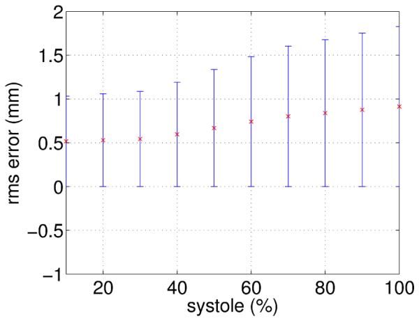
Intraobserver MSE error of manually placed landmarks at tag intersections.
Figure 14.

Tag distortion and its influence on the intraobserver error. A magnification of tags shows an ambiguity in point correspondence between ED (left) and ES (right) images. For the cross and circle at ED, there are two possible corresponding points at ES.
The initial pairwise registration of our method only provides a coarse initialization aiming to set the parameters inside the region of capture of the joint metric. After this initialization, the mean error is approximately 25% higher than the error provided by the method by Chandrashekara et al. (2004a) (1.32 0.12mm. and 1.06 0.12mm. respectively). After joint registration the error is 10% lower with respect to the same method of reference (0.95 ± 0.05mm.).
In this paper, the strain analysis was constrained to systole only because the tag fading precludes an accurate strain estimation beyond ES. Tag fading is quite strong in images acquired using SPAMM, and other sequences like CSPAMM have been developed to reduce this problem (Fischer et al., 1993). A priori, there are no apparent problems preventing the application of the presented method to the whole cardiac cycle. Similar data acquisition issues explain the exclusion of the right ventricle (RV) of the analysis. The minimum tag spacing provided by the scanner used in this paper was not sufficient to calculate strains accurately in the RV, but it could be included in the analysis in case of suitable image resolution is available.
There is an underestimation of the strain values reported in this paper. The first frame of the sequence is usually discarded since the blood is still magnetized in ED, and because of the presence of artifacts similar to those produced by off-resonance and velocity-induced phase discontinuities (Kim et al., 2003). As a consequence, the estimated strain values are lower than the real ones, and this could partially explain the differences found with the reported values in the literature. In our data, there are 10 frames during systole (in average), and therefore the discarded frames represent a loss of 103 approximately.
The strain values reported in the literature are very variable, which makes difficult a direct comparison to our results. This variability is a consequence of differences in the datasets and the estimation methods. An issue frequently disregarded is the presence of respiration artifacts and their implications on cardiac segmentation. Even when in this paper sequences presenting severe artifacts of this type were discarded, this problem is still present to some degree in all sequences, producing random local changes in the surface curvature (and therefore in the radial direction). On the contrary, circumferential direction is always in the plane of image acquisition, and does not change among subjects, which could explain the low variability of strain in this direction. Some methods to remove respiration artifacts in cMRI have been proposed (Chandler et al., 2006; Lötjönen et al., 2004), but they need to be modified for tMRI images. A possibility is to apply tag removal methods (Quian et al., 2007), before using the previously mentioned techniques.
Figures 10 and 11 show that HARP provides similar results with respect to the circumferential strain. However, the radial strain estimated by HARP shows some inhomogeneities over the left ventricle, with negative values in the inferior and inferolateral regions. In comparison, the presented method provided a more homogeneous distribution of the radial strain over systole, which is more consistent with the current knowledge of the cardiac physiology.
Note that the range of variation of the strain values is similar for HARP and our method (the color scales used in Figures 10 and 11 are exactly the same). The inclusion of the LA view is one of the sources of the differences obtained with respect to HARP, but it's not the only one because our method incorporates temporal information as well. Based on the experiments we have performed, we are unable to attribute the differences to a single source. We have compared both methods as a whole and a further analysis should be performed to fully answer this question.
Preliminary tests on patients with myocardial infarction showed an agreement between the recovered and expected strain. Full correspondence between infarcted regions and low strain values was found, in agreement with previous results from studies with 2D US (Becker et al., 2006; Chan et al., 2006; Jurcut et al., 2008; Sachdev et al., 2006; Vartdal et al., 2007; Zhang et al., 2005) and MRI (Garot et al., 2004; Geskin et al., 1998; Korosoglou et al., 2008; Spottiswoode et al., 2007). These experiments are only illustrative, and show consistent strains values compared to other modalities.
5. Conclusions
In this paper, we have used JA of tMRI sequences for cardiac motion estimation, motivated by the promising results reported for methods based on information-theoretic metrics, and from a probabilistic point of view in Section 2.3. To cope with the high computational cost of the kNNG estimators of Ha, an analytical expression for metric derivatives was obtained, resulting in a O(N l og N) complexity, which reduces drastically the registration time. The strategy to combine different views performed correctly, resulting in a simple way of integrating their information into a unified metric that measures multiphase and multiview similarity in image sequences. Results showed significantly lower mean errors and variances when compared to a standard PA approach. Strain values corresponding to healthy subjects were similar to those reported in the literature. However, the lack of standardization, and the high number of sources of variability, make a direct comparison difficult. Strain values for patients with myocardial infarction showed an excellent visual correlation with infarction location and territories at risk. Even when these results are encouraging, experiments need to be extended to a larger population to confirm and generalize clinical conclusions. In this paper, we have shown an interesting clinical application of graph-based metric estimators, showing their value for solving practical problems found in medical imaging.
6. Appendix: analytical derivatives
Many optimizers need to estimate the gradient of the cost function. To this purpose, the use of finite difference approximation to the gradient is impractical for transformations with high number of parameters, since it requires computing a kd-tree for each perturbation of the set of parameters. This is especially problematic for high-dimensional feature spaces as the number of perturbations requires for the finite difference estimator is D. This problem of graph-based estimators has been addressed by Sabuncu and Ramadge (2005) for Minimum Spanning Tree (MST) estimators of Ha Here we develop a similar analytical approximation.
Using Equation 6, the derivative with respect to the parameter m of the transformation is
| (13) |
The problem has been reduced to computation of derivatives . By assuming no changes in correspondence between a point z and its nearest neighbor for infinitesimal changes in the transformation parameters, these derivatives can be computed as:
| (14) |
where is the intensity gradient at the point xj = Tj(x), and is the mth column of the parametric jacobian of the transformation (Ibanez et al., 2008):
| (15) |
Finally, by including Equations 14 into Equation 13, the following expression is obtained for the derivative of the Ha:
| (16) |
It is important to highlight at this point, that Equation 13 is a completely general expression and can be used for any type of matching features. If zi are concatenations of features in JRd for each time point j, Equation 14 turns into
| (17) |
where ~7Zjk represents the spatial gradient of the kth feature coefficient at time j, and its computation depends on the feature definition.
By applying Equation 16 for computing derivatives, the time complexity is reduced to O(N log N) as compared to the O(N2 log N) time complexity required for finite differences.
Footnotes
The natural strain εN is defined as the integral over time of the instantaneous strain,
References
- Altman D. Practical Statistics for Medical Research. Chapman & Hall: 1997. [Google Scholar]
- Axel L, Montillo A, Kim D. Tagged magnetic resonance imaging of the heart: A survey. Med Image Anal. 2005 Aug;9(4):376–93. doi: 10.1016/j.media.2005.01.003. [DOI] [PubMed] [Google Scholar]
- Becker M, Bilke E, Kiihl H, Katoh M, Kramann R, Franke A, Biicker A, Hanrath P. Analysis of myocardial deformation based on pixel tracking in two dimensional echocardiographic images enables quantitative assessment of regional left ventricular function. Heart. 2006 Aug;92(8):1102–8. doi: 10.1136/hrt.2005.077107. R., H. [DOI] [PMC free article] [PubMed] [Google Scholar]
- Bellman RE. Dynamic programming. Dover Publications; Mineola, N.Y.: 2003. [Google Scholar]
- Belytschko T, Liu W, Moran B. Nonlinear Finite Elements for Continua and Structures. John Wiley & Sons; England: 2001. [Google Scholar]
- Cerqueira MD, Weissman NJ, Dilsizian V, Jacobs AK, Kaul S, Laskey WK, Pennell DJ, Rumberger JA, Ryan T, Verani MS. Standardized myocardial segmentation and nomenclature for tomographic imaging of the heart: a statement for healthcare professionals from the cardiac imaging committee of the council on clinical cardiology of the American Heart Association. Circulation. 2002 Jan;105(4):539–42. doi: 10.1161/hc0402.102975. [DOI] [PubMed] [Google Scholar]
- Chan J, Hanekom L, Wong C, Leano R, Cho G, Marwick T. Differentiation of subendocardial and transmural infarction using two-dimensional strain rate imaging to assess short-axis and long-axis myocardial function. J Am Coll Cardiol. 2006 Nov;48(10):2026–33. doi: 10.1016/j.jacc.2006.07.050. [DOI] [PubMed] [Google Scholar]
- Chandler AG, Pinder RJ, Netsch T, Schnabel JA, Hawkes DJ, Hill DLG, Razavi R. In: Third IEEE International Symposium on Biomedical Imaging: From Nano to Macro, ISBI. IEEE; Arlington, VA: Apr, 2006. 2006. Correction of misaligned slices in multi-slice MR cardiac examinations by using slice-to-volume registration; pp. 474–7. [Google Scholar]
- Chandrashekara R, Mohiaddin RH, Rueckert D. Analysis of 3D myocardial motion in tagged MR images using non rigid image registration. IEEE Trans Med Imag. 2004a Oct;23(10):1245–50. doi: 10.1109/TMI.2004.834607. [DOI] [PubMed] [Google Scholar]
- Chandrashekara R, Mohiaddin RH, Rueckert D. In: IEEE International Symposium on Biomedical Imaging: From Nano to Macro, ISBI. IEEE; Arlington, VA, USA: Apr, 2004b. 2004. Cardiac motion tracking in tagged MR images using a 4D B-spline motion model and nonrigid image registration; pp. 468–71. [Google Scholar]
- Cover TM, Thomas JA. Elements of information theory. Wiley-Interscience. 1991 [Google Scholar]
- Fischer SE, McKinnon GC, Maier SE, Boesiger P. Improved myocardial tagging contrast. Magnetic Resonance in Medicine. 1993 Aug;30(2):191–200. doi: 10.1002/mrm.1910300207. [DOI] [PubMed] [Google Scholar]
- Garot J, Lima JA, Gerber BL, Sampath S, Wu KC, Bluemke DA, Prince JL, Osman NF. Spatially resolved imaging of myocardial function with strain-encoded MR: comparison with delayed contrast-enhanced MR imaging after myocardial infarction. Radiology. 2004 Nov;233(2):596–602. doi: 10.1148/radiol.2332031676. [DOI] [PubMed] [Google Scholar]
- Geskin G, Kramer CM, Rogers WJ, Theobald M, Pakstis D, Hu YL, Reichek N. Quantitative assessment of myocardial viability after infarction by dobutamine magnetic resonance tagging. Circulation. 1998 Jul;98(3):217–23. doi: 10.1161/01.cir.98.3.217. [DOI] [PubMed] [Google Scholar]
- Hero AO, Costa J, Ma B. Tech. Rep. CSPL-334. Communications and Signal Processing Laboratory; The University of Michigan: Mar, 2003. Asymptotic relations between minimal graphs and alphα-entropy. [Google Scholar]
- Ibanez L, Schroeder W, Ng L, Cates J. The ITK software guide. 2008 Available at http://www.itk.org. [Google Scholar]
- Jurcut R, Pappas CJ, Masci PG, Herbots L, Szulik M, Bogaert J, Van de Werf F, Desmet W, Rademakers F, Voigt JU, D'hooge J. Detection of regional myocardial dysfunction in patients with acute myocardial infarction using velocity vector imaging. J Am Soc Echocardiogr. 2008 Aug;21(8):879–86. doi: 10.1016/j.echo.2008.02.002. [DOI] [PubMed] [Google Scholar]
- Kim D, Bove CM, Kramer CM, Epstein FH. Importance of k-space trajectory in echo-planar myocardial tagging at rest and during dobutamine stress. Magnetic Resonance in Medicine. 2003 Oct;50(4):813–20. doi: 10.1002/mrm.10589. [DOI] [PubMed] [Google Scholar]
- Korosoglou G, Youssef AA, Bilchick KC, Ibrahim E, Lardo AC, Lai S, Osman NF. Real-time fast strain-encoded magnetic resonance imaging to evaluate regional myocardial function at 3.0 Tesla: Comparison to conventional tagging. J Magn Reson Imaging. 2008 May;27(5):1012–8. doi: 10.1002/jmri.21315. [DOI] [PubMed] [Google Scholar]
- Learned-Miller EG. Data driven image models through continuous joint alignment. IEEE Trans. Pattern Anal. Machine Intell. 2006 Feb;28(2):236–50. doi: 10.1109/TPAMI.2006.34. [DOI] [PubMed] [Google Scholar]
- Ledesmα-Carbayo MJ, Kybic J, Desco M, Santos A, Suhling M, Hunziker P, Unser M. Spatio-temporal nonrigid registration for ultrasound cardiac motion estimation. IEEE Trans Med Imag. 2005 Sep;24(9):1113–26. doi: 10.1109/TMI.2005.852050. [DOI] [PubMed] [Google Scholar]
- Leonenko N, Pronzato L, Savani V. A class of Renyi information estimators for multidimensional densities. Annals of Statistics. 2008 Oct;36(5):2153–82. [Google Scholar]
- Lilliefors H. On the Komogorov-Smirnov test for normality with mean and variance unknown. J Am Stat Assoc. 1967;62:399–402. [Google Scholar]
- Lorensen W, Cline H. Marching cubes A high resolution 3D surface construction algorithm. Computer Graphics. 1987 Jul;4(21):163–9. [Google Scholar]
- Lotjonen J, Pollari M, Kivisto S, Lauerma K. Correction of movement artifacts from 4D cardiac short and long-axis MR data. In: Barillot C, Haynor DR, Hellier P, editors. Medical Image Computing and Computer-Assisted Intervention MICCAI 2004, 7th International Conference, Part II. Vol. 3217 of Lecture Notes in Computer Science. Springer; Saint-Malo, France: Sep, 2004. pp. 405–12. [Google Scholar]
- Ma B, Narayanan R, Park H, Hero AO, Bland PH, Meyer CR. Comparing pairwise and simultaneous joint registrations of decorrelating interval exams using entropic graphs. In: Karssemeijer N, Lelieveldt BPF, editors. Information Processing in Medical Imaging, 20th International Conference, IPMI 2007. Vol. 4584 of Lecture Notes in Computer Science. Springer; Kerkrade, The Netherlands: Jul, 2007. pp. 270–82. [DOI] [PMC free article] [PubMed] [Google Scholar]
- Moore CC, Lugo-Olivieri CH, McVeigh ER, Zerhouni EA. Three-dimensional systolic strain patterns in the normal human left ventricle: characterization with tagged MR imaging. Radiology. 2000 Feb;214(2):453–66. doi: 10.1148/radiology.214.2.r00fe17453. [DOI] [PMC free article] [PubMed] [Google Scholar]
- Mount DM. Department of Computer Science and Institute for Advanced Computer Studies. University of Maryland; College Park, Maryland: Aug, 2006. ANN programming manual. [Google Scholar]
- Neemuchwala H, Hero AO, Zabuawala S, Carson P. Image registration methods in high-dimensional space. Int J Imag Syst Tech. 2007;16(5):130–45. [Google Scholar]
- Neemuchwala HF, Hero AO. Multi-sensor image fusion and its applications. Marcel-Dekker, Ch. Entropic graphs for registration. 2005:185–235. [Google Scholar]
- Osman NF, Kerwin WS, McVeigh ER, Prince JL. Cardiac motion tracking using cine harmonic phase (HARP) magnetic resonance imaging. Magn Reson Med. 1999;42(6):1048–60. doi: 10.1002/(sici)1522-2594(199912)42:6<1048::aid-mrm9>3.0.co;2-m. [DOI] [PMC free article] [PubMed] [Google Scholar]
- Pai VM, Axel L. Advances in MRI tagging techniques for determining regional myocardial strain. Curr Cardiol Rep. 2006 Feb;8(1):53–8. doi: 10.1007/s11886-006-0011-4. [DOI] [PubMed] [Google Scholar]
- Petitjean C, Rougon N, Cluzel P. Assessment of myocadial function: a review of quantification methods and results using tagged MRI. J Cardiovasc Magn Reson. 2005 Apr;7(2):501–516. doi: 10.1081/jcmr-200053610. [DOI] [PubMed] [Google Scholar]
- Petitjean C, Rougon N, Preteux F, Cluzel P, Grenier P. Measuring myocardial deformations from MR data using informationtheoretic non rigid registration. In: Magnin IE, Montagnat J, Clarysse P, Nenonen J, Katila T, editors. Functional Imaging and Modeling of the Heart, Second International Workshop. Vol. 2674 of Lecture Notes in Computer Science. Springer; Lyon, France: Jun, 2003. pp. 162–72. [Google Scholar]
- Petitjean C, Rougon N, Preteux F, Cluzel P, Grenier P. Quantification of myocardial function using tagged MR and cine MR images. Int J Cardiovasc Imaging. 2004 Dec;20(6):497–507. doi: 10.1007/s10554-004-1098-6. [DOI] [PubMed] [Google Scholar]
- Quian Z, Huang R, Metaxas D, Axel L. Fouth IEEE International Symposium on Biomedical Imaging: From Nano to Macro, ISBI 2007. IEEE; Washington, USA: Apr, 2007. A novel tag removal technique for tagged cardiac MRI and its applications; pp. 364–7. [Google Scholar]
- Radeva P, Amini A, Huang J. Deformable B-solids and implicit snakes for 3D localization and tracking of SPAMM MRI data. Comput Vis Image Understand. 1997 May;66(2):163–78. [Google Scholar]
- Rao C. Linear Statistical Inference and Its Applications. 2nd Wiley; 2002. [Google Scholar]
- Redmond C, Yukich JE. Asymptotics for euclidean functionals with power-weighted edges. Stochastic Processes and their Applications. 1996 Feb;61(2):289–304. [Google Scholar]
- Renyi A. On measures of entropy and information. In: Neyman J, editor. Proceedings of the Fourth Berkeley Symposium on Mathematical Statistics and Probability. Vol. 1. University of California Press; Berkeley, CA, USA: Jun-Jul. 1961. pp. 547–61. [Google Scholar]
- Ripley BD. Pattern Recognition and Neural Networks. Cambridge University Press; Jan, 1996. [Google Scholar]
- Rutz AK, Ryf S, Plein S, Boesiger P, Kozerke S. Accelerated whole-heart 3D CSPAMM for myocardial motion quantification. Magn Reson Med. 2008 Apr;59(4):755–63. doi: 10.1002/mrm.21363. [DOI] [PubMed] [Google Scholar]
- Sabuncu MR, Ramadge PJ. IEEE International Conference on Acoustics, Speech, and Signal Processing. Vol. 2. Philadelphia, PA, USA: Mar, 2005. Gradient based optimization of an EMST image registration function; pp. 253–6. [Google Scholar]
- Sachdev V, Aletras AH, Padmanabhan S, Sidenko S, Rao YN, Brenneman CL, Shizukuda Y, Lie GR, Vincent PS, Waclawiw MA, Arai AE. Myocardial strain decreases with increasing transmurality of infarction: a Doppler echocardiographic and magnetic resonance correlation study. J Am Soc Echocardiogr. 2006 Jan;19(1):34–9. doi: 10.1016/j.echo.2005.07.013. [DOI] [PubMed] [Google Scholar]
- Schroeder W, Martin K, Lorensen B. The Visualization Toolkit, An Object Oriented Approach to 3D Graphics. Kitware Inc.; 1998. [Google Scholar]
- Shen D, Sundar H, Xue Z, Fan Y, Litt H. Consistent estimation of cardiac motion by 4D image registration. In: Duncan JS, Gerig G, editors. Medical Image Computing and Computer-Assisted Intervention - MICCAI 2005, 8th International Conference, Part II. Vol. 3750 of Lecture Notes in Computer Science. Springer; Palm Springs, CA, USA: Oct, 2005. pp. 902–10. [DOI] [PubMed] [Google Scholar]
- Spottiswoode BS, Zhong X, Hess A, Kramer CM, Meintjes EM, Mayosi BM, Epstein FH. Tracking myocardial motion from cine DENSE images using spatiotemporal phase unwrapping and temporal fitting. IEEE Trans Med Imag. 2007 Jan;26(1):15–30. doi: 10.1109/TMI.2006.884215. [DOI] [PubMed] [Google Scholar]
- Sutherland GR, Hatle L, Claus P, Dhooge J, Bijnens BH. Doppler Myocardial Imaging. (1st) 2006 BSWK. [Google Scholar]
- Vartdal , Brunvand, H., Pettersen E, Smith HJ, Lyseggen E, Helle-Valle T, Skulstad H, Ihlen H, Edvardsen T. Early prediction of infarct size by strain Doppler echocardiography after coronary reperfusion. J Am Coll Cardiol. 2007 Apr;49(16):1715–21. doi: 10.1016/j.jacc.2006.12.047. [DOI] [PubMed] [Google Scholar]
- Yukich JE. Probability theory of classical Euclidean optimization. Vol. 1675 of Lecture Notes in Mathematics. Springer-Verlag; Berlin: 1998. [Google Scholar]
- Zerhouni E, Parish D, Rogers W. Human heart: tagging with MR imaging - A method for non invasive assessment of myocardial motion. Radiology. 1988;169(1):59–63. doi: 10.1148/radiology.169.1.3420283. [DOI] [PubMed] [Google Scholar]
- Zhang Y, Chan AK, Yu CM, Yip GW, Fung JW, Lam WW, So NM, Wang M, Wu EB, Wong J, Sanderson JE. Strain rate imaging differentiates transmural from non-transmural myocardial infarction: a validation study using delayed-enhancement magnetic resonance imaging. J Am Coll Cardiol. 2005 Sep;46(5):864–71. doi: 10.1016/j.jacc.2005.05.054. [DOI] [PubMed] [Google Scholar]


