Catchment Area Analysis Using Bayesian Regression Modeling

Abstract

A catchment area (CA) is the geographic area and population from which a cancer center draws patients. Defining a CA allows a cancer center to describe its primary patient population and assess how well it meets the needs of cancer patients within the CA. A CA definition is required for cancer centers applying for National Cancer Institute (NCI)-designated cancer center status. In this research, we constructed both diagnosis and diagnosis/treatment CAs for the Massey Cancer Center (MCC) at Virginia Commonwealth University. We constructed diagnosis CAs for all cancers based on Virginia state cancer registry data and Bayesian hierarchical logistic regression models. We constructed a diagnosis/treatment CA using billing data from MCC and a Bayesian hierarchical Poisson regression model. To define CAs, we used exceedance probabilities for county random effects to assess unusual spatial clustering of patients diagnosed or treated at MCC after adjusting for important demographic covariates. We used the MCC CAs to compare patient characteristics inside and outside the CAs. Among cancer patients living within the MCC CA, patients diagnosed at MCC were more likely to be minority, female, uninsured, or on Medicaid.

Introduction

A National Cancer Institute (NCI)-designated cancer center is an important resource to its community and is mandated to decrease cancer incidence and mortality among populations within its catchment area (CA), including minority and underserved populations. A CA is the geographic area and population from which a cancer center draws patients. Defining a CA allows a medical center to describe its primary patient population and assess how well it meets the needs of patients within the CA. A CA should capture a significant portion of the hospital’s activity and exclude areas whose contribution to hospital activity probably represents random variation. It should also reflect geographical and demographic influences on hospital activity, including physical barriers to access and competition, and be proportional in geographic size to hospital size.¹ A defined CA is important for an NCI Cancer Center, as it is required as part of the application for the NCI Cancer Center Support Grant (CCSG) process. According to the NCI CCSG guidelines (February 19, 2013),² “the catchment area must be defined and justified by the center based on the geographic area it serves. It must be population based, eg, using census tracts, zip codes, county or state lines, or geographically defined boundaries. It must include the local area surrounding the cancer center.”

Several methods have been proposed in the literature to define CAs for a health center of interest. A simple approach has been used to define the CA based on a particular measure of distance from the center, where the area inside a particular distance threshold composes the CA. Examples of this approach include Luo and Qi,³ who use a fixed distance (eg, 30 miles) or a travel time based on a road network to define a CA. Luo and Whippo⁴ use a threshold-based population size to determine the distance for demarcating the CA. The main drawback of using this type of approach is that the threshold distance is deterministic and effectively arbitrary; it is not estimated from the observed data. Another approach using distance to define a CA is by Judge et al.⁵, who use Thiessen polygons to define a CA, where the Thiessen polygon for the center comprises all points in space that are closest to that center. This approach assumes that patients will travel to the facility that is closest in Euclidean space.

Another approach to defining a CA uses patient flow data to determine a distance to define the CA. For example, Phibbs and Robinson⁶ determined the distance radius that contained 75% or 90% of hospital patients. Alexandrescu et al.⁷ define a CA by selecting areas that cumulatively account for 80% of hospital patients. Baker⁸ selects areas that contained a threshold percent (eg, 0.5%) of the total facility activity. As with the distance-based approach, the main drawback of this approach is that the cumulative patient threshold (eg, 75% or 80% of patients) used to define the spatial boundary of the CA is not estimated from the data.

A different method proposed to define a CA is K-means clustering, which Gilmour¹ uses to define a CA for a large hospital in England based on three variables at the local authority district (LAD) level. Hospitals are run by Trusts in England, and for every Trust, a dataset of three variables was constructed, with one observation for each LAD that provided at least one patient admission to the hospital. The three variables were the proportion of hospital admissions coming from each LAD, the proportion of a LAD’s total admissions going to a given hospital, and the Euclidean distance between a hospital and an LAD. Separately for each Trust, the LAD data were divided into two clusters using K-means clustering with K = 2 to define a CA for each Trust. In K-means clustering, distance refers to the distance between observations in a Euclidean space with dimensions given by the variables of interest in the dataset, and variables need not be strictly based on geographic distance. One drawback of the use of this method as implemented in Gilmour¹ is that the clustering analysis did not include any area-level demographic or patient covariates. An advantage of the K-means approach compared with the previously described approaches is that it estimates the CA extent based on several variables at the area level instead of deterministically specifying the spatial extent of the CA based on geographic distance.

Another approach for CA delineation that estimates the extent of the CA is based on a method used in disease cluster analysis. Su et al.⁹ use the local spatial scan implemented in the software SaTScan¹⁰ to define a CA for the Sidney Kimmel Comprehensive Cancer Center (SKCCC) at Johns Hopkins based on Johns Hopkins Hospital cancer registry’s patient counts in counties in seven adjacent states and the District of Columbia. The local spatial scan is generally used to detect a contiguous geographic area that differs statistically in some quantity from the surrounding area. For disease analysis, it is used to detect geographic areas of statistically significantly elevated disease risk. A disadvantage of the local spatial scan is that the analysis must be stratified to adjust for any important confounders. Su et al.⁹ use a Poisson model as the base for the local spatial scan, with SKCCC patient counts in the numerator and total cancer deaths as the denominator (as a surrogate for the population with cancer) for the rate of SKCCC patient counts per cancer death for each county. Su et al created different CAs for gender, cancer site (colon or lung, breast, pancreas, prostate), age group (<18 years, 18+), and race (white, African American). One drawback of the analysis by Su et al is that they did not use state registry data, and hence, only consider patients who visited SKCCC when estimating the CA extent. The total population with cancer was not known.

Onyile et al.¹¹ also use the local spatial scan for creating a CA. Specifically, they use SaTScan to define a CA for a health information exchange in NYC, the New York Clinical Information Exchange (NYCLIX), with patient and census data from the three adjacent states of New York, New Jersey, and Connecticut. They use a Poisson model as the base model of the local spatial scan with the number of NYCLIX patients in each county and the number of people living in each county according to the 2010 census to calculate the relative risk of visiting the NYCLIX facility. They define the CA as a group of adjacent counties that each had a relative risk greater than 1. One limitation of the analysis in Onyile et al.¹¹ is that they did not use state registry data, but only patient data from the NYCLIX and at-risk population data from the U.S. Census.

The previously described approaches to creating a catchment center for a health center each have their advantages, including ease of use, and disadvantages, including a lack of a statistical inference framework or the ability to account for covariates in the CA analysis. As an alternative, we propose to apply Bayesian hierarchical regression models to create CAs for a large health center. The Bayesian regression framework allows one to estimate a probability-based CA while making statistical inference and adjusting for patient demographic variables. Our objective in this work is to create CAs for a large cancer center, Massey Cancer Center (MCC) at the Virginia Commonwealth University Health System (VCUHS), which is seeking comprehensive cancer status from NCI. We used data from two different sources to construct a diagnosis CA for all cancers from state cancer registry data (Virginia Cancer Registry, VCR) and a diagnosis/treatment CA using patient billing data from MCC.

Methods

Study data

VCR data

We obtained records from VCR for all diagnosed cancer patients during years 2009–2011 living in the state of Virginia at the time of diagnosis. Ethical approval for the study was granted by the IRB of Virginia Commonwealth University. The VCR data included demographic variables gender, race, age, health insurance type, reporting hospital, and residential ZIP code at the time of diagnosis or treatment. Originally, the data contained 160,307 records and 124,609 patients for the three years of study. We detected and deleted duplicated records for the same patient with the same cancer, tumor site, and diagnosed date, which was because of reporting of the same cancer for the same patient by different hospitals. After excluding duplicated records and records with missing values, we included 124,819 records and 118,452 patients in the CA analysis. Of those patients, 6,286 (5.3%) patients were diagnosed at MCC according to the reporting hospital coded in the VCR data.

MCC data

We obtained billing record data from MCC for all cancer patients diagnosed or treated at MCC during the period 2009–2012. The MCC data included demographic variables such as gender, race, date of birth, and health insurance type and address at the time of diagnosis or treatment. The data contained 28,873 patients, of which 28,317 lived in the State of Virginia at the time of diagnosis or treatment at MCC. Of the 28,317 records, there were 24,576 records for treatment or diagnosis during the period 2009–2011. After excluding records with missing values for race, there were 24,537 patients diagnosed or treated at MCC during period 2009–2011 and 28,242 patients diagnosed or treated at MCC during period 2009–2012 who were included in the CA analysis.

Statistical analysis

We used the cancer patient data from the two data sources to create two types of CAs. We first used the state cancer registry (VCR) data to create a CA map for diagnosis at MCC during 2009–2011. We then used the VCUHS billing data (MCC data) to create CA maps for diagnosis or treatment at MCC during 2009–2011 and during 2009–2012. The first diagnosis/treatment CA analysis was limited in time (2009–2011) to correspond with the temporal range of VCR data, and the second diagnosis/treatment CA analysis (2009–2012) was intended to identify any change over time in the CA. For each patient dataset, we aggregated the data spatially to the county level to facilitate models with population subgroups based on patient demographics. CAs based on units smaller than a county were not of interest for the research presented here.

We used Bayesian hierarchical logistic regression to model the proportion of diagnosed cancer patients in each county in Virginia who were diagnosed at MCC during 2009–2011. The demographic variables of patient race, gender, and age were included in the logistic regression model to evaluate the relationship between the odds of diagnosis at MCC and patient characteristics. Random effects for counties were included to model residual variation in the odds of being diagnosed at MCC after adjusting for the demographic variables. We specified the logistic regression model as

$$\log \left(\frac{p_{ij}}{1-p_{ij}}\right)={\beta }_0+{\beta }_{1}Mal{e}_{ij}+{\beta }_{2}Ag{e}_{ij}+{\beta }_{3}Blac{k}_{ij}+{\beta }_{3}Othe{r}_{ij}+{\nu }_i,$$ (1)

where p_ij is the probability of diagnosis at MCC for cancer patients located in the county i with covariate pattern j,(i = 1,…,134, j = 1,…,12), and v_i is the county-specific random effect. The covariate patterns were defined by combinations of the demographic variables male (female as the reference level), age group of 65+ years (0–64 years as the reference level), and black and other non-white race (white as the reference level).

We considered two different priors for the random effects. The first was an exchangeable prior, which treats the random effects as independent, and the second was an intrinsic conditional autoregressive (CAR) prior,¹² which assumes that random effects are correlated among neighboring counties, v_i ~ CAR (τ), where τ is the precision. The intrinsic CAR distribution may be expressed as

$${\nu }_i|{\nu }_{(l\ne i)}~N(({\overline{\nu }}_i),(1)/(m_i\tau )),$$ (2)

where m_i is the number of adjacent counties for county i. The conditional mean of the distribution is ${\overline{\nu }}_i={\displaystyle \sum _{lin{\delta }_i}{\nu }_l}$, where δ_i is the set of neighbors adjacent to county i. The deviance information criterion (DIC) is used for comparing the goodness-of-fit of Bayesian models. Models with smaller DIC are better than those with larger DIC.¹³ The exchangeable prior model had a meaningfully lower DIC value than the CAR prior, and we report results below only for the exchangeable prior model.

To model the rate of diagnosis or treatment at MCC, we used a Bayesian hierarchical Poisson regression model with the count of patients diagnosed or treated for cancer at MCC and a measure of the at-risk population count in each county. In order to see if the CA changed with additional data over time, we fitted separate Poisson regression models based on MCC data during 2009–2011 and MCC data during 2009–2012. The population data to represent the at-risk population were population counts by population subgroups from the 2010 U.S. Census. The demographic variable of black or other non-white race, with white as the reference level, was included in the model. Population counts were only available for individual covariates (not cross-tabulations of covariates), and we elected to adjust for one of the covariates most likely to be associated with diagnosis or treatment at MCC. Random effects for counties were included to model residual risk of being diagnosed or treated for cancer at MCC after adjusting for race. We specified the Poisson regression model hierarchically as

$$\begin{array}{l}{Y}_{ij}~Poisson\left({\mu }_{ij}\right),\\ {\mu }_{ij}=e_{ij}\times R_{ij},\\ \log \left(R_{ij}\right)={\beta }_0+{\beta }_{1}Blac{k}_{ij}+{\beta }_{2}Othe{r}_{ij}+{\nu }_i,\end{array}$$ (3)

where Y_ij is the count of MCC-diagnosed/treated patients in county i with race j, μ_ij is the unknown mean count, e_ij is the expected count of MCC-diagnosed/treated patients in county i with race j over all counties, R_ij is the relative risk of population diagnosed or treated at MCC in county i with race j(i = 1,…,134, j = 1, 2,3), and ν_i is the county-specific random effect. The expected count e_ij was calculated as the count of MCC-diagnosed/treated patients with race j for all counties divided by the population with race j for all counties and then multiplied by the population in county i with race j. We again considered models with an exchangeable prior and with an intrinsic CAR prior. The exchangeable prior had the lower DIC, and we report results from this model below.

For the priors for the logistic and Poisson models, the prior distribution for the intercept was an improper uniform prior dflat distribution, and the priors for the covariate regression coefficients were Normal (0,10⁻⁵), where 10⁻⁵ represents the precision. The exchangeable prior for the random effects was normal with mean zero and precision τ₁, which had a Gamma (0.5,0.0005) prior. The CAR prior for the random effects had a precision τ₂ that had a Gamma (0.5,0.0005) prior. The priors were selected to be conjugate priors.

We fitted the Bayesian regression models using R version 3.0.0 software¹⁴ with package R2WinBUGS.¹⁵ In the Markov chain Monte Carlo (MCMC) procedure to estimate model parameters, we used two chains with a burn-in period of 10,000 iterations and G = 10,000 subsequent samples from the joint posterior distribution to calculate posterior mean estimates of the parameters for each model. Convergence of each model was assessed by the Brooks–Gelman–Rubin statistic,¹⁶ where a value about 1 is considered as an indicator of convergence of the MCMC.

To define CAs for MCC, we used exceedance probabilities to assess unusual clustering of patients going to MCC. The exceedance probability is defined as q_i = Pr (θ_i > 1), which is an estimate of how frequently the odds ratio (OR) (logistic model) or the relative risk (Poisson model) exceeds the null value (θ_i = 1). Under posterior sampling using MCMC, a converged sample of $\{{\theta }^{m+1},\dots ,{\theta }^{m+m_p}\}$ can yield posterior expected estimates of these probabilities as

$${\widehat{q}}_i={\displaystyle \sum _{g=m+1}^{m+m_p}\frac{I\left({\theta }_i^{(g)}>1\right)}{G}},$$ (4)

where G = m_p and m is the number of burn-in samples. For the logistic model, the estimated OR for each county was calculated as exp (ν_i − mean(ν_i)) where mean(ν_i) is the mean of ν_i over all counties. For the Poisson model, the estimated relative risk for each county was directly obtained from the output of posterior sample simulation. The threshold of exceedance probabilities to define the CA was ${\widehat{q}}_i>0.90$. In other words, a county was marked as inside the CA if its exceedance probability was greater than 0.90. The threshold of 0.90 is a conventional value in calculating exceedance probabilities in disease mapping.¹⁷ We also tried different threshold values for the exceedance probability, including values of 0.80, 0.85, and 0.95. For the Poisson model, the CA was first created for each stratum of the demographic variable. A final CA for the Poisson model was constructed as a conflation of counties marked for inclusion in any of the stratum CAs. In other words, if a county was included in any stratum CA, it was included in the final CA.

For a comparison with our Bayesian regression methods, we also applied K- means clustering and the local spatial scan to both VCR and MCC datasets in the time period 2009–2011. We did not adjust for demographic covariates with K-means clustering and the local spatial scan. The three variables for K-means clustering were the proportion of MCC patients coming from each county, the proportion of a county’s cancer patients going to MCC, and the Euclidean distance between MCC and a county centroid. For the local spatial scan, we used a Poisson model as the base model of the local spatial scan with the number of Massey patients in each county and the number of cancer people in each county (for VCR dataset) or the total population in each county according to the 2010 census (for MCC dataset) to calculate the relative risk of visiting MCC.

Results

Diagnosis CA

The regression parameter estimates and associated ORs for the Bayesian logistic model are shown in Table 1. All coefficients were significant at the level 0.05. Men had lower risk of being diagnosing at MCC than women, with an estimated OR of 0.88 (95% CI: 0.83, 0.93). Older patients (65+ years) had lower risk of being diagnosing at MCC than younger patients (<65 year), with an estimated OR of 0.42 (95% CI: 0.40, 0.45). Blacks and those of other non-white race had higher risk of being diagnosing at MCC than whites, with estimated OR of 1.52 (95% CI: 1.42, 1.62) and 1.27 (95% CI: 1.04, 1.54), respectively. Hence, blacks were over 1.5 times more likely to be diagnosed at MCC than whites.

Table 1.

Parameter estimates from the Bayesian logistic regression model for diagnosis CA based on VCR data.

VARIABLE	COEFFICIENT	SE	95% CI	P-VALUE	OR	CI FOR OR
Intercept	−3.79	0.198	(−4.18, −3.40)	<0.0001	–	–
Male	−0.13	0.029	(−0.19, −0.08)	<0.0001	0.88	(0.83, 0.93)
Age2 (≥65)	−0.86	0.030	(−0.92, −0.80)	<0.0001	0.42	(0.40, 0.45)
Black	0.42	0.032	(0.35, 0.48)	<0.0001	1.52	(1.42, 1.62)
Other	0.24	0.101	(0.04, 0.43)	0.0175	1.27	(1.04, 1.54)

Abbreviations: SE, standard error; CI, confidence interval; OR, odds ratio.

The CA map for diagnosis at MCC is shown in Figure 1 using an exceedance probability threshold of 0.90. In all, 54 out of 134 counties in Virginia were included in the CA. The CA is centered in Richmond, as expected, and consists of a contiguous set of counties, along with the Eastern Shore of Virginia counties Northampton and Accomack. We also mapped the exceedance probabilities estimated from the Bayesian logistic regression model (Fig. 2) to show that the definition of the CA is not heavily dependent on the exceedance probability threshold value. The number of counties in the estimated CA using the exceedance probability thresholds of 0.80, 0.85, and 0.95 were 57, 54, and 53, respectively. For the following results, we used the threshold of 0.90.

Figure 1.

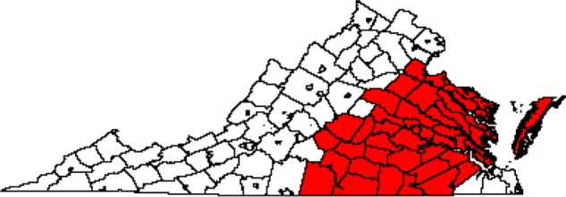
CA for diagnosis at MCC based on VCR data during 2009–2011 for all cancers (n = 54 counties).

Figure 2.

Map of exceedance probabilities for diagnosis at MCC based on VCR data during 2009–2011 for all cancers.

Table 2 shows the number of all diagnosed cancer patients inside the CA and the number of MCC-diagnosed patients inside the diagnosis CA for all cancers. Among 11,303 diagnosed black patients inside the diagnosis CA, 2,173 (19.2%) patients were diagnosed at MCC. In contrast, MCC served 12.1% of white patients diagnosed with cancer inside the CA. From this table, we see that MCC has served a relatively large proportion of those aged less than 65 years (19.1%) as well as patients who are black (19.2%), of other race (19.2%), Hispanic (30.9%), uninsured (41.5%), or on Medicaid (33.9%). Hence, MCC has been a center of cancer diagnosis for the traditionally underserved populations of minorities and uninsured patients.

Table 2.

Total number of diagnosed cancer patients and MCC-diagnosed patients inside the diagnosis CA for all cancers.

PATIENT GROUPS		TOTAL PATIENTS	MCC PATIENTS	PERCENT MCC
Gender	Male	20301	2635	13.0%
	Female	20677	3177	15.4%
Age	Age (<65)	20084	3830	19.1%
	Age (≥65)	20894	1982	9.5%
Race	White	29042	3526	12.1%
	Black	11303	2173	19.2%
	Other	633	113	17.9%
Hispanic	Yes	2341	723	30.9%
	No	38637	5089	13.2%
Insurance	Not insured	1591	660	41.5%
	Medicaid	1227	416	33.9%
	Medicare	18083	2025	11.2%
	Other	1400	62	4.4%
	Unknown	2802	158	5.6%
	Private	15875	2491	15.7%

Table 3 shows characteristics of cancer patients diagnosed at MCC versus those not diagnosed at MCC, both inside and outside the MCC diagnosis CA for all cancers. Table 4 shows patient characteristics inside and outside the diagnosis CA for all cancers. Comparing these two tables, we see that 27.6% of patients inside the CA but not diagnosed at MCC were black, while 37.4% of the MCC patients inside the CA were black. Outside the CA, 13.6% of patients not diagnosed at MCC were black, while 25.5% of MCC patients were black. Therefore, MCC has served a greater proportion of black patients both inside and outside the diagnosis CA. This is also true for younger patients, uninsured patients, and those on Medicaid. Inside the CA, there were higher proportions of patients diagnosed at MCC who were younger (65.9%), uninsured (11.2%), and on Medicaid (7.2%) than those younger (46.2%), uninsured (2.6%), and on Medicaid (2.3%) not diagnosed at MCC.

Table 3.

Patient characteristics for diagnosis CA for MCC based on VCR data for all cancers. Percent values are based on numbers within each column.

PATIENT GROUPS		MCC PATIENTS INSIDE CA (%)	NON-MCC PATIENTS INSIDE CA (%)	MCC PATIENTS OUTSIDE CA (%)	NON-MCC PATIENTS OUTSIDE CA (%)
Gender	Male	2635 (45.3%)	17666 (50.2%)	230 (52.4%)	34937 (46.3%)
	Female	3177 (54.7%)	17500 (49.8%)	209 (47.6%)	40502 (53.7%)
Age	Age (<65)	3830 (65.9%)	16254 (46.2%)	350 (79.7%)	37738 (50.0%)
	Age (≥65)	1982 (34.1%)	18912 (53.8%)	89 (20.3%)	37701 (50.0%)
Race	White	3526 (60.7%)	25516 (72.6%)	309 (70.4%)	61991 (82.2%)
	Black	2173 (37.4%)	9130 (26.0%)	112 (25.5%)	10218 (13.5%)
	Other	113 (1.9%)	520 (1.5%)	18 (4.1%)	3230 (4.3%)
Hispanic	Yes	723 (12.4%)	1618 (4.6%)	47 (10.7%)	9956 (13.2%)
	No	5089 (87.6%)	33548 (95.4%)	392 (89.3%)	65483 (86.8%)
Insurance	Not insured	650 (11.2%)	931 (2.6%)	58 (13.2%)	2932 (3.9%)
	Medicaid	416 (7.2%)	811 (2.3%)	50 (11.4%)	2428 (3.2%)
	Medicare	2025 (34.8%)	16058 (45.7%)	105 (23.9%)	31718 (42.0%)
	Other	62 (1.1%)	1338 (3.8%)	10 (2.3%)	2236 (3.0%)
	Unknown	158 (2.7%)	2644 (7.5%)	8 (1.8%)	5363 (7.1%)
	Private	2491 (43.0%)	13384 (38.1%)	208 (47.4%)	30762 (40.8%)

Table 4.

Patient characteristics for diagnosis CA for MCC based on VCR data for all cancers. Percent values are based on the numbers within each column.

PATIENT GROUPS		ALL PATIENTS INSIDE CA (%)	ALL PATIENTS OUTSIDE CA (%)
Gender	Male	20301 (49.5%)	35167 (46.3%)
	Female	20677 (50.5%)	40711 (53.7%)
Age	Age (<65)	20084(49.0%)	38088 (50.2%)
	Age (≥65)	20894 (50.1%)	37790 (49.8%)
Race	White	29042 (70.9%)	62300 (82.1%)
	Black	11303 (27.6%)	10330 (13.6%)
	Other	633 (1.5%)	3248 (4.3%)
Hispanic	Yes	2341 (5.7%)	10003 (13.2%)
	No	38637 (94.3%)	65875 (86.8%)
Insurance	Not insured	1591 (3.9%)	2990 (3.9%)
	Medicaid	1277 (3.0%)	2478 (3.3%)
	Medicare	18083 (44.1%)	31823 (41.9%)
	Other	1400 (3.4%)	2246 (3.0%)
	Unknown	2802 (6.8%)	5371 (7.1%)
	Private	15875 (38.7%)	30970 (40.8%)

Diagnosis/treatment CA

The CA for diagnosis/treatment at MCC is shown in Figure 3 for 2009–2011 and in Figure 4 for 2009–2012. There were 44 out of 134 counties in Virginia included in the CA for diagnosis/treatment in 2009–2011, while 47 counties were included in the 2009–2012 CA. As with the diagnosis CA for 2009–2011, the diagnosis/treatment CAs were centered on the city Richmond and were contiguous, with the exception of the inclusion of part of the Eastern Shore in 2009–2012. The CA increased in size by three counties when including data for 2012, suggesting that MCC expanded its service area over time. Specifically, the CA expanded slightly to the east and to the north. The 2009–2012 CA added part of the Eastern Shore to the 2009–2011 CA, and it added a county in northern Virginia. The county membership for all three CAs is listed in Supplementary Table 1.

Figure 3.

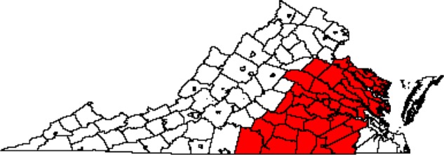
CA for diagnosis/treatment for MCC based on MCC data in 2009–2011 for all cancers (n = 44 counties).

Figure 4.

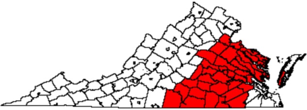
CA for diagnosis/treatment for MCC based on MCC data in 2009–2012 for all cancers (n = 47 counties).

Though similar in shape to the diagnosis CA during 2009–2011, the diagnosis/treatment CAs for 2009–2011 and 2009–2012 are slightly smaller in spatial extent. For example, for 2009–2011, the diagnosis/treatment CA does not include any counties composing the Eastern Shore, and for 2009–2012, it only includes one of the two counties composing the Eastern Shore. The diagnosis/treatment CAs also include two fewer counties on the western border of the CA. Even with these few differences, the diagnosis and diagnosis/treatment CAs are remarkably similar, despite being derived from two different datasets and statistical models.

Table 5 shows the number of MCC patients inside and outside the diagnosis/treatment CA for MCC in 2009–2012. Inside the CA, 30.4% of MCC-diagnosed/treated patients were black, while outside the CA, 25.3% of MCC-diagnosed/treated patients were black. Therefore, MCC has served a greater proportion of black patients inside the diagnosis/treatment CA than outside the CA during 2009–2012. There are also higher proportions of females (59.8%), older patients (39.4%), and those on Medicare (40.1%) diagnosed/treated at MCC inside the CA than females (50.1%), older patients (26.8%), and those on Medicare (29.5%) diagnosed/treated at MCC outside the CA.

Table 5.

Patient characteristics for 2009–2012 diagnosis/treatment CA for MCC based on MCC data. Percent values are based on the numbers within each column.

PATIENT GROUPS		MCC PATIENTS INSIDE CA (%)	MCC PATIENTS OUTSIDE CA (%)
Gender	Male	10278 (40.2%)	1333 (49.9%)
	Female	15290 (59.8%)	1341 (50.1%)
Age	Age (<65)	15490 (60.6%)	1957 (73.2%)
	Age (≥65)	10078 (39.4%)	717 (26.8%)
Race	White	16784 (65.6%)	1849 (69.1%)
	Black	7773 (30.4%)	676 (25.3%)
	Other	1011 (4.0%)	149 (15.8%)
Insurance	Not insured	2300 (9.0%)	348 (13.0%)
	Medicaid	3017 (11.8%)	356 (13.3%)
	Medicare	10252 (40.1%)	789 (29.5%)
	Other	436 (1.7%)	127 (4.7%)
	Unknown	47 (0.2%)	6 (0.2%)
	Private	9476 (37.1%)	1048 (39.2%)

Table 6 shows the total number of MCC-diagnosed/treated cancer patients and the number of MCC-diagnosed/treated cancer patients inside the CA for 2009–2012. From Table 6, we can see that 92.0% of MCC-diagnosed/treated black patients and 93.4% of MCC-diagnosed/treated older patients were captured inside the CA. Therefore, the diagnosis/treatment CA during 2009–2012 captures a relatively large proportion of MCC-diagnosed/treated patients.

Table 6.

Total number of MCC-diagnosed/treated cancer patients and total number of MCC-diagnosed/treated cancer patients inside 2009–2012 diagnosis/treatment CA based on MCC data.

PATIENT GROUPS		TOTAL MCC PATIENTS	MCC PATIENTS INSIDE CA	PERCENTAGE INSIDE CA
Gender	Male	11611	10278	88.5%
	Female	16631	15290	91.9%
Age	Age (<65)	17447	15490	88.8%
	Age (≥65)	10795	10078	93.4%
Race	White	18633	16784	90.1%
	Black	8449	7773	92.0%
	Other	1160	1011	87.2%
Insurance	Not insured	2648	2300	86.9%
	Medicaid	3373	3017	89.4%
	Medicare	11041	10252	92.9%
	Other	563	436	77.4%
	Unknown	53	47	88.7%
	Private	10524	9476	90.0%

The diagnosis CA maps based on K-means clustering and the local spatial scan are shown in Figures 5 and 6. The number of counties included in the CAs was 30 for K-means clustering and 42 for the local spatial scan. The diagnosis/treatment CA maps based on K-means clustering and the local spatial scan are shown in Figures 7 and 8. The number of counties included in the CAs was 33 for K-means clustering and 41 for the local spatial scan. Compared with our Bayesian model diagnosis and diagnosis/treatment CAs, which contained 54 and 44 counties, respectively, we see that K-means clustering and the local spatial scan yielded smaller CAs. The CAs overlap spatially to the extent that the Bayesian CAs effectively contain not only the CAs estimated from K-means clustering and the local spatial scan but also adjacent counties.

Figure 5.

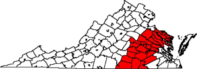
CA map for diagnosis at MCC based on VCR data during 2009–2011 for all cancers using K-means clustering (n = 30 counties).

Figure 6.

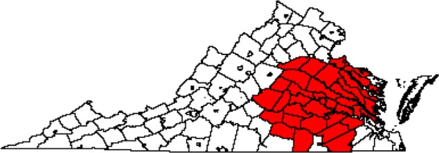
CA map for diagnosis at MCC based on VCR data during 2009–2011 for all cancers using the local spatial scan (n = 42 counties).

Figure 7.

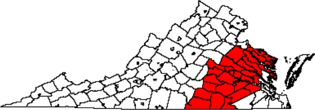
CA for diagnosis/treatment for MCC based on MCC data in 2009–2011 for all cancers using K-means clustering (n = 33 counties).

Figure 8.

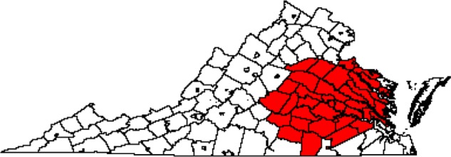
CA for diagnosis/treatment for MCC based on MCC data in 2009–2011 for all cancers using the local spatial scan (n = 41 counties).

Discussion and Conclusion

We used Bayesian hierarchical regression models to estimate diagnosis and diagnosis/treatment CAs for MCC using state cancer registry data, hospital billing data, and census data at the county level. Our results showed that the CAs for MCC were fairly large (n = 54 for diagnosis, n = 44 or 47 for diagnosis/treatment), reflecting the significant presence of this large, urban cancer center in Virginia. The diagnosis/treatment CA increased slightly in size from 2009–2011 to 2009–2012. We also found that MCC has served a large proportion of black, Hispanic, and uninsured patients, and those on Medicaid. In addition to its large presence, MCC has played an important role as a care provider for traditionally underserved populations of cancer patients.

While the Bayesian hierarchical regression framework is well established, the application of these methods for defining CAs is novel. Existing methods for defining a CA are not probability based, may require a priori selection of a distance or patient flow threshold, or do not adjust easily for covariates. In contrast with previously proposed and applied approaches for CA analysis, the Bayesian regression models can estimate the CA stochastically from the data using exceedance probabilities, while adjusting for several covariates. Estimating effects for patient demographics were beneficial for understanding differences in the likelihood of being seen at MCC according to patient characteristics. For example, we found that non-white patients were significantly more likely to be diagnosed at MCC than white patients. In addition, we could handle different types of available data with different forms of the regression model. Also, we could evaluate the benefit of including a prior on random effects that assume spatial correlation across counties by comparing a Bayesian measure of goodness-of-fit. In our case, including a spatially correlated prior for county effects was unnecessary because of the strong spatial signal present in the patient data for being seen at MCC.

One limitation of our method is that the models are limited in the number of population group strata they can include. For example, if we increased the number of categorical variables in the logistic model, we encountered a number of strata in some counties that had zero counts for cancer patients. The zero counts are problematic in the denominator when modeling the proportion. One solution is to add a small constant to the patient counts, but this artificially augments the data. Another solution is to adjust for a small number (relative to the number of observations) of categorical covariates. Yet another solution is to model data on an individual level, when available, which we will explore in future work. Another obstacle encountered when working with cancer registry data is multiple reporting of cancers by different hospitals or duplication of cancer records. The presence of such records requires additional data processing steps and the ability to identify unique patients through a unique identifier or a combination of variables, including diagnosis date, cancer type, tumor site, age, gender, race, etc. In addition, the cancer registry data do not include all types of cancer. For example, skin cancer is not reported to the VCR. However, diagnosis or treatment for skin cancer is captured in hospital billing records. While we could work with cancer registry data and hospital billing data separately, differences in composition of the cancer cases and covariates made it infeasible to use the data in combination.

Despite these limitations and obstacles, we were able to demonstrate the utility of applying Bayesian hierarchical regression models to define multiple CAs for a large cancer center. This framework for estimating CAs should be applicable to other large hospitals.

Supplementary File

Supplementary Table 1

County membership in three catchment areas (CA). Diagnosis catchment area was determined from Virginia Cancer Registry data. Diagnosis/treatment catchment area was determined from Virginia Commonwealth University Health System billing data.

REFERENCES

- 1.Gilmour SJ. Identification of hospital catchment areas using clustering: an example from the NHS. Health Serv Res. 2010;45(2):497–513. doi: 10.1111/j.1475-6773.2009.01069.x. [DOI] [PMC free article] [PubMed] [Google Scholar]
- 2.National Institutes of Health, National Cancer Institute, Office of Cancer Centers Policies and guidelines relating to the P 30 Cancer Center Support Grant. 2013. pp. 1–56. Available at: http://cancercenters.cancer.gov/documents/ccsg_guidelines.pdf.
- 3.Luo W, Qi Y. An enhanced two-step floating catchment area (E2SFCA) method for measuring spatial accessibility to primary care physicians. Health Place. 2009;15:1100–7. doi: 10.1016/j.healthplace.2009.06.002. [DOI] [PubMed] [Google Scholar]
- 4.Luo W, Whippo T. Variable catchment sizes for the two-step floating catchment area (2SFCA) method. Health Place. 2012;18:789–95. doi: 10.1016/j.healthplace.2012.04.002. [DOI] [PubMed] [Google Scholar]
- 5.Judge A, Welton NJ, Sandhu J, Ben-Shlomo Y. Geographical variation in the provision of elective primary hip and knee replacement: the role of socio-demographic, hospital and distance variables. J Public Health. 2009;31(3):413–22. doi: 10.1093/pubmed/fdp061. [DOI] [PubMed] [Google Scholar]
- 6.Phibbs CS, Robinson JC. A variable-radius measure of local hospital market structure. Health Serv Res. 1993;28(3):313–24. [PMC free article] [PubMed] [Google Scholar]
- 7.Alexandrescu R, O’Brien SJ, Lyons RA, Lecky FE. A proposed approach in defining population-based rates of major injury from a trauma registry dataset: delineation of hospital catchment areas (I) BMC Health Serv Res. 2008(8):80. doi: 10.1186/1472-6963-8-80. [DOI] [PMC free article] [PubMed] [Google Scholar]
- 8.Baker LC. Measuring competition in health care markets. Health Serv Res. 2001;36(1):223–51. [PMC free article] [PubMed] [Google Scholar]
- 9.Su SC, Kanarek N, Fox MG, Guseynova A, Crow S, Ouabtadisum S. Spatial analyses identify the geographic source of patients at a National Cancer Institute Comprehensive Cancer Center. Clin Cancer Res. 2010;16(3):1065–72. doi: 10.1158/1078-0432.CCR-09-1875. [DOI] [PubMed] [Google Scholar]
- 10.Kulldorff M. A spatial scan statistic. Commun Stat. 1997;26:1481–96. [Google Scholar]
- 11.Onyile A, Vaidya SR, Kuperman G, Shapiro JS. Geographical distribution of patients visiting a health information exchange in New York City. J Am Med Inform Assoc. 2012;20:125–30. doi: 10.1136/amiajnl-2012-001217. [DOI] [PMC free article] [PubMed] [Google Scholar]
- 12.Besag J, York J, Mollie A. Bayesian image restoration, with two applications in spatial statistics (with discussion) Annals Inst Stat Math. 1991;43:1–59. [Google Scholar]
- 13.Spiegelhalter DJ, Best NG, Carlin BP, van der Linde A. Bayesian measures of model complexity and fit (with discussion) J R Stat Soc B. 2002;64:583–640. [Google Scholar]
- 14.R Development Core Team . R: A Language and Environment for Statistical Computing. Vienna, Austria: R Foundation for Statistical Computing; 2008. [Google Scholar]
- 15.Sturtz S, Ligges U, Gelman A. R2WinBUGS: A Package for Running Win-BUGS from R. Journal of Statistical Software. 2005;12(3):1–16. [Google Scholar]
- 16.Brooks SP, Gelman A. General methods for monitoring convergence of iterative simulations. J Comput Graph Stat. 1998;7(4):434–55. [Google Scholar]
- 17.Lawson A. Bayesian Disease Mapping: Hierarchical Modeling in Spatial Epidemiology, Second Edition. London: CRC Press; 2013. [Google Scholar]
Associated Data
This section collects any data citations, data availability statements, or supplementary materials included in this article.
Supplementary Materials